Abstract
This study evaluates the positional accuracy of Global Navigation Satellite Systems (GNSS) and Unmanned Aerial vehicle (UAV)-based LiDAR systems in terrain modeling, using a total station as a reference. The research was conducted over 17 Ground Control Points (GCPs), with measurements obtained using a CHCNAV i50 GNSS receiver and a DJI Zenmuse L1 Light Detection and Ranging (LiDAR) sensor mounted on a UAV. Accuracy was assessed for horizontal (X, Y) and vertical (Z) components by comparing the results against total station data. Errors were quantified using statistical metrics such as Mean Absolute Error (MAE), Root Mean Square Error (RMSE), and RMS at 1σ. GNSS exhibited superior horizontal accuracy with an RMS 1σ of 1.1 cm, while LiDAR achieved 1.7 cm. In contrast, GNSS outperformed LiDAR in vertical precision, achieving a 1σ RMS of 6.4 cm compared to 6.6 cm for LiDAR. These findings align with manufacturer specifications and international standards such as those of the American Society for Photogrammetry and Remote Sensing (ASPRS). The results highlight that GNSS is preferable for applications requiring high horizontal precision, while LiDAR is better suited for vertical modeling and terrain analysis. The combination of both systems may offer enhanced results for comprehensive geospatial surveys. Overall, both technologies demonstrated sub-decimetric accuracy suitable for precision agriculture, civil engineering, and environmental monitoring.
1. Introduction
The evolution of topographic surveying techniques has enabled the transition from traditional methods to advanced technological solutions that optimize the capture and processing of spatial data. In this context, GNSS and LiDAR technology have revolutionized terrain modeling, providing geospatial data with high precision and spatial resolution, while also increasing data capture resolution and speed [1]. These technologies have proven to be essential tools in multiple disciplines, ranging from territorial planning and environmental management to precision agriculture and civil engineering [2]. However, the increasing availability of these technologies has sparked debates regarding the actual accuracy of the models generated compared to those obtained through conventional methods, such as the use of total stations [3]. However, GNSS accuracy can be affected by systematic and environmental errors, such as ionospheric and tropospheric disturbances and satellite geometry [4]. On the other hand, LiDAR enables the acquisition of three-dimensional data by emitting laser pulses and measuring the signal return time, allowing the generation of high-resolution digital elevation models [5,6]. This technology has been particularly useful in applications where dense vegetation cover hinders the use of conventional photogrammetric methods [7].
Despite advancements in GNSS and LiDAR, evaluating their accuracy remains a critical topic in geospatial research. Mesbah et al. [8] reports that errors in terrain modeling can be quantified using statistical metrics such as RMSE and MAE, which allow comparisons between deviations in generated models and reference values obtained through more conventional and validated methods, such as total stations. Previous studies as Pérez et al. [9] and Garzón Barrero et al. [10] have shown that while LiDAR is highly efficient for capturing large areas in a short time, it can present positioning errors due to georeferencing quality, laser return density, and post-processing techniques used. Similarly, GNSS accuracy depends on the type of receiver used, observation time, and the availability of differential corrections [11].
The use of these technologies in precision agriculture has been the subject of recent research, highlighting their applicability in generating terrain models to optimize soil and crop management [12]. However, the combination of GNSS and LiDAR in agricultural environments still faces challenges related to data calibration and the spatial variability of terrains [13]. In civil engineering, LiDAR has been widely employed in detecting structural deformations and infrastructure planning, where its integration with GNSS has enhanced the accuracy of three-dimensional models [14]. To determine the reliability of these technologies in terrain modeling, rigorous comparisons with traditional topographic methods are essential. Various studies have implemented hybrid approaches that combine GNSS, LiDAR, and total station data to improve the accuracy of geospatial models [15]. The standardization of these procedures is key to ensuring the replicability of results and their applicability in different contexts [16].
This study aims to evaluate the accuracy of GNSS and LiDAR systems in terrain modeling compared to traditional topographic methods. To achieve this, measurements were conducted in an experimental area using a drone equipped with a LiDAR sensor, GNSS receivers and a total station as a high-precision reference. Through statistical metric analysis, the differences in accuracy between the evaluated technologies were determined to establish objective criteria for their implementation in geospatial applications.
2. Materials and Methods
2.1. Study Area
The study was conducted at the training ground of the School of Agricultural Engineering of the Technological Institute of Costa Rica (9°51′8” N, 83°54′35” W) (Figure 1). The study area covers 800 m2, average elevation is 1407 m above sea level and had an average slope of 5%. At the time of data collection, there was no bare soil cover, and the soil texture was clayey.
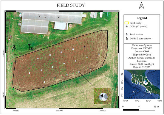
Figure 1.
Study area map.
The remote sensing data and field samples were captured on 16 October 2024. For the land point collection, 17 targets were used, arranged in an equidistant grid of 5 × 5 m. LiDAR data was acquired using a DJI Zenmuse L1 laser scanner [17]. This sensor was mounted on DJI Matrice 300 UAV [18]. The positional accuracy of the system was increased by incorporating Real Time Kinematic GNSS techniques using the DJI D-RTK2 differential correction base station [19]. The coordinates of the GCPs were captured using a CHCNAV i50 GNSS receiver [20] and a CHCNAV CTS-112R4 total station [21].
2.2. Data Acquisition
The GCPs were designed with an alternating black-and-white quadrant pattern (Figure 2a), characterized by high-contrast divisions centered at a single point [22]. This configuration was selected to optimize the visual recognition of the geometric center, thereby improving the precision and consistency of spatial measurements in both terrestrial and aerial surveys. The distinct contrast between quadrants facilitates automated and manual detection processes, reducing potential errors during data acquisition and post-processing [23].
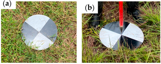
Figure 2.
GCPs used. (a) Design of the targets, (b) geometric center where X, Y, Z coordinates will be obtained.
To ensure homogeneous spatial coverage and adequately represent the conditions of the terrain, a total of 17 GCPs were placed in three rows. The first row consisted of 5 GCPs, the second of 7, and the third of 5. This staggered pattern (5-7-5) was designed to optimize the distribution of the GCPs across the experimental area, minimizing potential biases in measurements due to spatial variations [24]. The row-based arrangement ensured that measurement points were well distributed, promoting data homogeneity while also facilitating access and repeatability of the measurements [25]. This approach was key to controlling spatial variability in the experiments and obtaining representative data from the entire study area, enabling precise comparison of the accuracy of the measurement systems used.
Each target was anchored to the ground using a 40 cm rod to ensure stability and was leveled both vertically and transversally. To avoid potential displacement during data collection, GNSS and total station measurements were completed prior to the UAV overflight. For data acquisition, the coordinates measured with the total station were used as the reference parameter. To georeference the base point where the station was positioned, static data collection was conducted using the CHCNAV i50 GNSS base [20]. The GNSS data were then post-processed using CGO software (v.2.2.2.11) [26], with a base station and the EGM2008 geoid model to calculate accurate coordinates, including altitude correction referenced to sea level [27]. The UAV LiDAR survey was performed at a flight altitude of 60 m with a flight path oriented at 80° relative to north. The LiDAR sensor was configured to record three returns per emitted pulse. Flight planning incorporated 70% forward overlap and 60% side overlap to guarantee sufficient redundancy for point cloud generation. GNSS/IMU corrections embedded in the trajectory were refined during processing in DJI Terra, and 17 GCPs were used to align the LiDAR trajectory and ensure accurate georeferencing.
Data Acquisition and Post-Processing of Static GNSS Bases
To establish a reliable geodetic reference, a static GNSS survey was performed at the base points used for georeferencing, leaving one as a master control point and two additional ones for total station orientation. Data were collected using a CHCNAV i50 GNSS receiver operating in static mode over a continuous observation period of 4 h. The raw RINEX files were processed in CHCNAV CGO2 software (v.2.2.2.11) [26], using differential baseline corrections from the two closest Continuous Operation Reference Station (CORS) stations, which corrected satellite ephemeris, clock bias, and atmospheric errors through static relative positioning differential corrections obtained from the Costa Rican Continuously Operating Reference Stations (CORS) network.
The two closest CORS stations, located approximately 21 km (San José, province of Costa Rica) and 98 km (Limón, province of Costa Rica) [28] from the study site, were used as reference bases. Processing was carried out using the CRTM05 coordinate system and the EGM2008 geoid model to transform ellipsoidal heights into orthometric heights [29].
2.3. Method
To evaluate the accuracy of GNSS and LiDAR technologies compared to traditional topographic methods, a comparative analysis was conducted based on horizontal and vertical discrepancies. Horizontal accuracy was assessed using the differences in the X and Y coordinates, while vertical accuracy focused on variations in the Z coordinate. The coordinates measured with the total station served as reference values. By comparing these with those obtained through GNSS and LiDAR, both the planimetric and altimetric precision of each system were quantified [30]. This method provided a clear understanding of positional deviations across the different measurement technologies. (Figure 3) shows the comparison graphically.
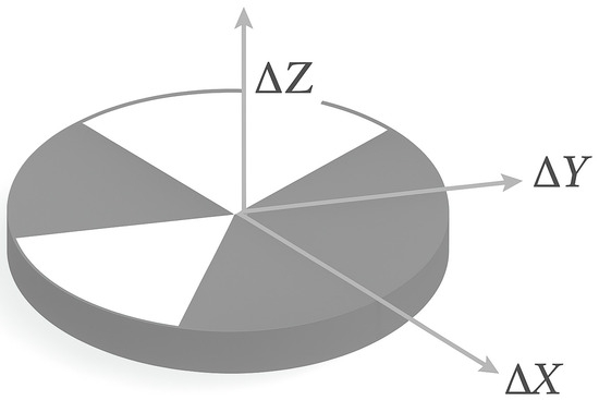
Figure 3.
Graphical representation of the error. In horizontal (ΔX, ΔY) and vertical (ΔZ).
2.4. Spatial Data Preparation
The foundation of this study was the construction of a comprehensive data table containing the X, Y, and Z coordinates obtained from each measurement method: GNSS, LiDAR, and total station. This table served as the primary dataset for evaluating the spatial accuracy of each system. Coordinates were organized to allow direct comparison between predicted values (GNSS and LiDAR) and reference values (total station). This structured format enabled the application of statistical metrics to assess horizontal and vertical differences across all observation points.
2.4.1. Georeferencing of Total Station Data
For the georeferencing of the total station data, the post-processed GNSS base point obtained in the previous step was used as the primary reference. From this base point, the total station setup was anchored to the geodetic framework. In addition, the two additional GNSS points were measured using static observations and processed against the same CORS-based solution. These two points were employed to calculate an azimuth, which allowed the accurate orientation of the total station. By assigning this reference and orientation, all measurements captured by the total station were transformed into georeferenced coordinates within the CRTM05 metric coordinate system, officially used in Costa Rica [31]. This procedure ensured spatial consistency across all measurements and enabled the integration of GNSS, LiDAR, and total station data into a unified geodetic framework. The use of a standardized coordinate system was essential to achieve compatibility between datasets and to perform reliable spatial comparisons throughout the analysis.
2.4.2. Preparation and Georeferencing of GNSS Data
For the preparation of the GNSS dataset, coordinate data were collected using a CHCNAV i50 receiver configured in real-time kinematic (RTK) mode, with differential corrections provided by a fixed base station. All measurements were taken at the same target points used for the total station and LiDAR surveys to ensure spatial correspondence. The raw GNSS data were subsequently post-processed using CGO software (v.2.2.2.11) [26], applying the EGM2008 geoid model [27] to correct the altimetric values and converting them to orthometric heights. The resulting dataset was transformed into the CRTM05 coordinate system [31], ensuring compatibility with the other data sources. This process provided high-precision georeferenced coordinates and allowed for a consistent assessment of horizontal and vertical accuracy compared to the reference dataset.
2.4.3. LiDAR Data Processing and Extraction of Target Coordinates
For the extraction of coordinates from the LiDAR survey, the raw point cloud was initially generated using DJI Terra (v.3.5.5) [32], the proprietary software designed for processing data collected by DJI UAVs equipped with LiDAR sensors. This software reconstructed the 3D environment and produced a dense point cloud representing the terrain and objects within the survey area. Following this, the point cloud was imported into TerraSolid (v. 023.026) [33], a specialized suite of tools for LiDAR data processing, where it underwent a classification process. This classification was performed using an RGB-based vegetation index method [34], which analyzes the red, green, and blue values associated with each point to distinguish vegetated surfaces from artificial or non-vegetated targets. This technique enabled the effective isolation of the high-contrast GCP targets from the surrounding vegetation and ground features.
Once the classification was completed, only the points corresponding to the GCP targets were retained. From each of these classified clusters, the centroidal coordinate—the geometric center of the target point group—was calculated using QGIS’s spatial analysis tools [35]. This centroid represented the most accurate X, Y, and Z position of each target as captured by the LiDAR sensor. The final set of centroidal coordinates was then compiled into a structured dataset for comparative analysis against the GNSS and total station measurements.
2.5. Quantitative Evaluation of Model Performance
The quantitative evaluation of the accuracy of the models generated by GNSS and LiDAR systems was carried out using two widely accepted statistical metrics in geospatial validation studies: MAE and RMSE. These metrics allow for a direct comparison between the values obtained from the evaluated sensors and the reference values captured using a total station, which is considered a high-precision measurement method [36].
MAE is defined as the average of the absolute errors, while RMSE is the square root of the average of the squared errors. The formulas used for their calculation were as follows [37]:
where N is the total number of observations, Pi represents the value obtained by the sensor (GNSS and LiDAR), and Oi corresponds to the observed reference value obtained with the total station. RMS 1σ corresponds to the standard deviation of errors around the mean, indicating the internal consistency of measurements. Unlike MAE and RMSE, which describe accuracy relative to reference values, RMS 1σ quantifies precision by assessing error dispersion.
Both metrics were computed separately for the horizontal components (X and Y coordinates) and the vertical component (Z coordinate), in order to distinguish the behavior of errors in each spatial dimension. This distinction is essential for identifying whether discrepancies are predominantly horizontal or vertical, which is particularly relevant for applications where vertical accuracy is critical, such as terrain modeling [38].
The selection of MAE and RMSE is based on their standardized use in the scientific literature for evaluating the accuracy of predictive models and spatial measurement systems both metrics provides a more comprehensive view of model performance, as RMSE is more sensitive to large errors due to its quadratic penalty, while MAE offers a more robust measure in the presence of outliers [36].
In MATLAB (v. R2023b), the Statistics and Machine Learning Toolbox [39] was used to compute the MAE and RMSE metrics based on the Equations (1) and (2). The input data consisted of tables with X, Y, and Z coordinates from GNSS, LiDAR, and total station measurements. The differences between predicted (Pi) and observed (Oi) values were processed using MATLAB’s built-in mean and sqrt functions [39] to calculate the MAE and RMSE values, enabling a comprehensive evaluation of model accuracy.
3. Results
The accuracy analysis using GNSS and LiDAR systems, compared to a high-precision total station, revealed notable differences in spatial precision. The evaluation focused on the horizontal components (X, Y) and the vertical component (Z), across a network of 17 regularly spaced GCPs within the study area. Errors were calculated by comparing the coordinates obtained from GNSS and LiDAR sensors with those from the total station, which served as the reference dataset. This comparison allowed quantification of absolute deviations and variability, essential for assessing the performance of each system in geospatial applications. The static GNSS data collected at the base point were post-processed against two CORS stations of the Costa Rican national geodetic network: San José (21 km from the study site) and Limón (98 km). Baseline processing was carried out using CHCNAV CGO2 software (v.2.2.2.11), applying the CRTM05 coordinate system and the EGM2008 geoid model to obtain orthometric heights. The post-processing results indicated that the derived base point coordinates achieved sub-centimetric horizontal precision and centimeter-level vertical precision. The values are shown in Table 1.

Table 1.
Horizontal and vertical precision of GNSS static points (in meters).
For the total station orientation, the azimuth was determined from the coordinates of the two additional GNSS static points. The difference between the measured horizontal angle and the theoretical azimuth derived from GNSS coordinates was calculated. The resulting angular deviation was 0.0014 rad (≈0.08°). This low value confirms that the total station was correctly aligned with the geodetic framework, ensuring consistency across all measurements.
A visual representation of the errors is provided in Figure 4, which shows the positional discrepancies in a stacked bar format. The vertical deviations observed at points D6–D12 showed a symmetrical distribution; however, this behavior did not follow a consistent pattern in the rest of the dataset and therefore does not indicate a systematic error. For each GCP, a single bar is displayed where the contribution of GNSS is shown in black and that of LiDAR in light gray. This format enables direct comparison of horizontal and vertical positional errors across technologies. The top panel corresponds to horizontal errors (computed as the Euclidean distance in the X and Y components), while the bottom panel displays the absolute vertical error in the Z coordinate. This graphic representation reveals the spatial behavior of each technology and identifies points where one system outperformed the other.
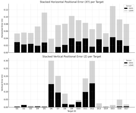
Figure 4.
Graphical representation of the error.
The distribution of errors across the control points demonstrates that GNSS generally maintains better performance in horizontal positioning, with most values remaining below 0.05 m. In contrast, LiDAR exhibits slightly larger deviations in the same dimension, particularly in areas where the scanning angle or vegetation cover may have interfered with laser return. The vertical error values show more complex trends due to the wide range in errors for both GNSS and LiDAR. These tendencies align with the inherent characteristics of both technologies: GNSS is affected by satellite geometry and atmospheric conditions, whereas LiDAR depends on point density, target reflectivity, and scan configuration. Errors were assessed using MAE and RMSE, as described in the Methods section. Table 2 presents the results for both horizontal and vertical dimensions.
Table 2.
MAE and RMSE of horizontal and vertical components (in meters).
These results corroborate the graphical trends observed. GNSS shows superior performance in horizontal accuracy, with lower MAE and RMSE values. Its average horizontal RMSE of 0.032 m reflects sub-decimetric precision, suitable for most precision mapping applications. Meanwhile, LiDAR, although less precise in planimetric terms, shows an advantage in vertical precision, with a slightly lower RMSE in the Z component (0.054 m vs. 0.064 m). This finding is particularly relevant for applications such as surface modeling or drainage mapping, where accurate representation of terrain elevation is critical.
In addition to error magnitude, evaluating the variability of positional errors provides further insight into the reliability of each system. For this, the 1σ Root Mean Square (RMS) deviation was calculated, aggregating the dispersion of errors by horizontal and vertical dimensions. The results are shown in Table 3.
Table 3.
1σ Root Mean Square (RMS) deviation for horizontal and vertical errors (in meters).
The horizontal RMS (1σ) values confirm the consistency of GNSS in horizontal positioning, exhibiting low dispersion (0.011 m) relative to LiDAR (0.017 m). This reaffirms GNSS’s advantage under favorable satellite geometry and open-sky conditions. However, the vertical RMS tells a different story: LiDAR delivers more stable elevation data (0.064 m) compared to GNSS (0.066 m), likely due to its capacity to capture denser point clouds with minimal vertical offset when properly georeferenced.
These findings underscore the importance of evaluating both accuracy and precision when selecting a terrain modeling technology. While GNSS provides a more uniform horizontal performance, LiDAR offers a clear advantage in vertical stability. The combination of both systems, with proper integration and calibration, may yield enhanced accuracy in both spatial dimensions particularly valuable in applications such as precision agriculture, hydrological modeling, and civil infrastructure planning.
4. Discussion
4.1. Static Data Processing
The post-processed static GNSS solution of the base point, referenced to two CORS stations (San José 21 km and Limón 98 km), achieved a horizontal precision of ±0.008 m and a vertical precision of ±0.015 m. These values are consistent with geodetic-grade standards and align with previously reported accuracies for static GNSS surveys using CORS networks, typically ranging from 0.5–1.5 cm horizontally and 1–2 cm vertically [40]. This reliability ensured that the georeferencing of total station, RTK-GNSS, and UAV LiDAR data was not compromised by reference errors. As emphasized by the ASPRS standards, a robust control framework is essential to avoid systematic distortions during multi-sensor integration. By anchoring the total station to a static solution and orienting it with an azimuth derived from two known GNSS points, the study minimized coordinate system shifts. This approach provided a stable reference, strengthening the validity of the subsequent accuracy comparisons.
4.2. Horizontal Accuracy Assessment
The results of this study show that the GNSS system achieved a horizontal RMS 1σ of 1.1 cm while the LiDAR system presented a value of 1.7 cm. These figures are consistent with manufacturer specifications and international accuracy standards under ideal conditions [41]. In light of manufacturer specifications, the empirical results observed in this study are consistent with the expected performance of the instruments used. The DJI Zenmuse L1 LiDAR sensor is reported to achieve a horizontal accuracy of ≤10 cm at a 1σ confidence level (approximately 68%) [17]. In comparison, the CHCNAV i50 GNSS receiver in RTK mode specifies accuracy of approximately 9 mm horizontally under similar confidence conditions [42]. The measured results 1.7 cm RMS (1σ) for LiDAR, and 1.1 cm for GNSS demonstrate that while the GNSS receiver performed slightly below its theoretical vertical precision, both systems operated well within their horizontal tolerances. These small deviations are attributable to environmental and operational factors inherent to field deployments, such as GNSS signal multipath, scan angle distortions in LiDAR, and post-processing variations. This suggests sub-centimeter horizontal accuracy is achievable in optimal settings. Although our GNSS results are slightly higher, they are reasonable given real-world field conditions where atmospheric interference and satellite geometry can impact precision [43].
4.3. Vertical Accuracy Assessment
In the vertical dimension, LiDAR showed a clear advantage with a 1σ RMS of 6.6 cm, compared to 6.4 cm for GNSS. This difference may be attributed to the ability of LiDAR to collect dense point clouds that model topographic surfaces more precisely. Studies showthat absolute vertical accuracy for LiDAR data should meet a RMSEz of 10 cm in open, flat terrain for topographic mapping [44]. The vertical RMSE obtained in our study 6.6 cm for LiDAR—not only satisfies but exceeds this requirement, suggesting high-quality data acquisition and processing procedures. For GNSS, vertical accuracy is more sensitive to error sources such as tropospheric delay and poor satellite geometry. Although the 6.4 cm vertical RMS slightly exceeds the specifications of some commercial GNSS receivers, it remains within acceptable bounds for most land surveys and mapping applications that do not demand sub-centimeter elevation accuracy [45].
4.4. Comparison with Previous Studies
Previous studies support the performance patterns observed in this work. For instance, in research evaluating GNSS receivers for precision agriculture, horizontal RMS values of around 2.7 cm and vertical errors of 5.1 cm were reported [43]. These findings align well with the GNSS performance documented here.
Similarly, other studies have shown that under optimal conditions, LiDAR can achieve vertical accuracies as fine as 2.5 cm (1σ). However, in realistic environments, where terrain complexity and vegetation are present, higher vertical RMS values—such as the 5.4 cm obtained in this study—are not only expected but remain highly satisfactory for digital terrain modeling (DTM) applications.
4.5. Practical Implications
Choosing between GNSS and LiDAR systems depends on project requirements, terrain complexity, and available resources. The findings of this study suggest that GNSS systems are well-suited for applications where high horizontal precision is essential, such as cadastral surveying, infrastructure layout, and boundary demarcation [46].
In contrast, LiDAR is advantageous in scenarios where vertical detail and surface modeling are critical, such as watershed analysis, erosion monitoring, and topographic modeling in forested areas. The consistent performance of LiDAR in the vertical dimension highlights its utility for generating high-resolution digital elevation models, especially when dense vegetation limits the applicability of photogrammetry or GNSS-only approaches [47].
5. Conclusions
This study evaluated the positional accuracy of GNSS and UAV-based LiDAR systems, using a total station as a reference. By using a static GNSS base point post-processed against CORS stations, the study ensured a geodetic-grade reference with sub-centimetric horizontal and centimeter-level vertical accuracy. This robust control minimized potential coordinate shifts and guaranteed that accuracy differences between GNSS, LiDAR, and total station measurements reflected the true performance of each technology, strengthening the reliability of the comparative analysis. By analyzing both horizontal (X, Y) and vertical (Z) components across 17 ground control points, a comprehensive comparison was conducted under realistic field conditions. The results demonstrate that GNSS outperformed LiDAR in horizontal accuracy, achieving a 1σ RMS of 1.1 cm compared to 1.7 cm for LiDAR. This supports the established use of RTK-GNSS for high-precision planimetric measurements, especially in applications where consistent horizontal control is essential.
Conversely, LiDAR exhibited superior vertical performance, with a vertical RMS of 5.4 cm, slightly lower than the 6.4 cm observed for GNSS. This aligns with LiDAR’s known capability to generate dense, high-resolution 3D surface data and confirms its reliability for digital elevation modeling, particularly in environments where photogrammetry or GNSS are limited by vegetation or terrain occlusion. Furthermore, both systems produced sub-decimetric accuracy in their respective strengths, with all results falling within or exceeding international mapping standards such as those proposed by ASPRS. The RMS and MAE values observed are also consistent with reported values in scientific literature, further validating the measurement protocols and integration strategies used.
In conclusion, each system presents specific advantages depending on the intended application: GNSS is preferred for high-accuracy horizontal positioning, while LiDAR is recommended for detailed vertical terrain representation. For comprehensive geospatial modeling, especially in agricultural or civil engineering contexts, a hybrid approach combining both technologies may provide optimal results, balancing planimetric consistency and vertical detail.
Author Contributions
Conceptualization, K.F.R. and Y.C.; methodology, K.F.R., Y.C., M.Q., Y.Z. and J.C.J.; software, K.F.R.; formal analysis, K.F.R.; writing—original draft preparation, K.F.R., Y.C. and M.Q.; writing—review and editing.; supervision, K.F.R.; project administration, K.F.R.; funding acquisition, K.F.R. All authors have read and agreed to the published version of the manuscript.
Funding
This research was funded by the Vice-Rectorate of Research and Outreach of the Costa Rica Institute of Technology, in support of the student project entitled: “La precisión en el modelamiento del terreno: una comparación entre equipos geodésicos, sensores remotos y de agrimensura”.
Data Availability Statement
The raw data supporting the conclusions of this article will be made available by the authors on request.
Acknowledgments
To the School of Agricultural Engineering of the Instituto Tecnologico de Costa Rica for support in data acquisition.
Conflicts of Interest
The authors declare no conflicts of interest.
References
- Tamimi, R.; Toth, C. Accuracy Assessment of UAV LiDAR Compared to Traditional Total Station for Geospatial Data Collection in Land Surveying Contexts. Int. Arch. Photogramm. Remote Sens. Spat. Inf. Sci. 2024, XLVIII-2-2024, 421–426. [Google Scholar] [CrossRef]
- Ade, M.; Harahap, K.; Wakkang, H.; Oktavio, A.; Mitasari, R.; Nugraha, A.R.; Triantho, A.I. Geopatial Technologies in Civil Engineering: A Critical Literature. Indones. J. Eng. Educ. Technol. (IJEET) 2024, 2, 274–281. [Google Scholar] [CrossRef]
- Khalil, R. The Accuracy of GIS Tools for Transforming Assumed Total Station Surveys to Real World Coordinates. J. Geogr. Inf. Syst. 2013, 5, 486–491. [Google Scholar] [CrossRef]
- Yan, Z.; Zheng, W.; Wu, F.; Wang, C.; Zhu, H.; Xu, A. Correction of Atmospheric Delay Error of Airborne and Spaceborne GNSS-R Sea Surface Altimetry. Front. Earth Sci. 2022, 10, 730551. [Google Scholar] [CrossRef]
- Wang, J.; Wu, Y.; Zhang, Y.; Lizaga, I.; Zhang, Z.; Papadopoulou, E.E.; Papakonstantinou, A. Combining Drone LiDAR and Virtual Reality Geovisualizations towards a Cartographic Approach to Visualize Flooding Scenarios. Drones 2024, 8, 398. [Google Scholar] [CrossRef]
- Omasa, K.; Hosoi, F.; Uenishi, T.M.; Shimizu, Y.; Akiyama, Y. Three-Dimensional Modeling of an Urban Park and Trees by Combined Airborne and Portable on-Ground Scanning LIDAR Remote Sensing. Environ. Model. Assess. 2008, 13, 473–481. [Google Scholar] [CrossRef]
- Małyszek, H.; Stachula, S.; Kępowicz, B. The Case Study of Using Photogrammetric Systems and Laser Scanning for Three-Dimensional Modeling of Cultural Heritage Sites. Adv. Sci. Technol. Res. J. 2023, 17, 345–357. [Google Scholar] [CrossRef]
- Mesbah, S.; Madbouly, M.M.; Ghanem, M. Error Assessment and Propagation in Digital Terrain Modeling: A Review. Int. Arch. Photogramm. Remote Sens. Spat. Inf. Sci. 2023, XLVIII-1/W2-2023, 611–617. [Google Scholar] [CrossRef]
- Pérez, J.J.; Senderos, M.; Casado, A.; Leon, I. Field Work’s Optimization for the Digital Capture of Large University Campuses, Combining Various Techniques of Massive Point Capture. Buildings 2022, 12, 380. [Google Scholar] [CrossRef]
- Barrero, J.G.; Burbano, C.E.C.; Jiménez-Cleves, G. Cuantificación Del Efecto de La Densidad de Datos de LiDAR En La Calidad Del DEM. Cienc. Ing. Neogranad. 2021, 31, 149–169. [Google Scholar] [CrossRef]
- Dizon, R.D.; Peñales, J.J.; Reyes, R.B.; Mabaquiao, L.C. Real-Time Water Level Monitoring Using Low-Cost Gnss Receiver. Int. Arch. Photogramm. Remote Sens. Spat. Inf. Sci. 2024, XLVIII-4-W8-2023, 189–194. [Google Scholar] [CrossRef]
- Sharma, S. Precision Agriculture: Reviewing the Advancements, Technologies, and Applications in Precision Agriculture for Improved Crop Productivity and Resource Management. Rev. Food Agric. (RFNA) 2023, 4, 45–49. [Google Scholar] [CrossRef]
- Manish, R.; Habib, A. In-Situ Calibration and Trajectory Enhancement of UAV LiDAR Systems for Mapping Mechanized Agricultural Fields. IEEE J. Sel. Top. Appl. Earth Obs. Remote Sens. 2024, 17, 7460–7474. [Google Scholar] [CrossRef]
- Baek, J. Two-Dimensional LiDAR Sensor-Based Three-Dimensional Point Cloud Modeling Method for Identification of Anomalies inside Tube Structures for Future Hypersonic Transportation. Sensors 2020, 20, 7235. [Google Scholar] [CrossRef]
- Du, M.; Li, H.; Roshanianfard, A. Design and Experimental Study on an Innovative UAV-LiDAR Topographic Mapping System for Precision Land Levelling. Drones 2022, 6, 403. [Google Scholar] [CrossRef]
- Deibe, D.; Amor, M.; Doallo, R. Big Data Geospatial Processing for Massive Aerial LiDAR Datasets. Remote Sens. 2020, 12, 719. [Google Scholar] [CrossRef]
- Support for Zenmuse L1-DJI. Available online: https://www.dji.com/global/support/product/zenmuse-l1 (accessed on 1 April 2025).
- Support for Matrice 300 RTK-DJI. Available online: https://www.dji.com/global/support/product/matrice-300 (accessed on 1 April 2025).
- DJI D-RTK High Precision GNSS Mobile Station. Available online: https://www.dji.com/ca/d-rtk-2 (accessed on 1 April 2025).
- CHCNAV GNSS I50. Available online: https://chcnav.es/productos/gps-chc-i50-gnss/chc-manual-gps-centimetrico-i50-es.pdf (accessed on 1 April 2025).
- CTS-112R4: Budget-Friendly Reflectorless Total Station|CHCNAV. Available online: https://geospatial.chcnav.com/products/chcnav-CTS-112R4 (accessed on 1 April 2025).
- Štroner, M.; Urban, R.; Línková, L. A New Method for UAV Lidar Precision Testing Used for the Evaluation of an Affordable DJI ZENMUSE L1 Scanner. Remote Sens. 2021, 13, 4811. [Google Scholar] [CrossRef]
- Štroner, M.; Urban, R.; Seidl, J.; Reindl, T.; Brouček, J. Photogrammetry Using UAV-Mounted GNSS RTK: Georeferencing Strategies without GCPs. Remote Sens. 2021, 13, 1336. [Google Scholar] [CrossRef]
- Tan, C.; Chen, Z.; Liao, A.; Zeng, X.; Cao, J. Accuracy Analysis of UAV Aerial Photogrammetry Based on RTK Mode, Flight Altitude, and Number of GCPs. Meas. Sci. Technol. 2024, 35, 106310. [Google Scholar] [CrossRef]
- Ferrer-González, E.; Agüera-Vega, F.; Carvajal-Ramírez, F.; Martínez-Carricondo, P. UAV Photogrammetry Accuracy Assessment for Corridor Mapping Based on the Number and Distribution of Ground Control Points. Remote Sens. 2020, 12, 2447. [Google Scholar] [CrossRef]
- CGO2: Advanced GNSS Post-Processing Software|CHCNAV. Available online: https://geospatial.chcnav.com/products/chcnav-CGO (accessed on 9 May 2025).
- Falchi, U.; Parente, C.; Prezioso, G. Global Geoid Adjustment on Local Area for GIS Applications Using GNSS Permanent Station Coordinates. Geod. Cartogr. 2018, 44, 80–88. [Google Scholar] [CrossRef]
- Estaciones SIRGAS de Costa Rica. Available online: https://www.arcgis.com/apps/View/index.html?appid=55a6a5db20de4b4d999364e56d2fa207 (accessed on 25 August 2025).
- Tavasci, L.; Vecchi, E.; Gandolfi, S. Definition of the Local Geoid Undulation Using Non-Contemporary GNSS-Levelling Data on Subsidence Area: Application on the Adriatic Coastline. Commun. Comput. Inf. Sci. 2022, 1507 CCIS, 259–270. [Google Scholar] [CrossRef]
- Pham, C.K.; Tran, D.T.; Nguyen, V.H. GNSS/CORS-Based Technology for Real-Time Monitoring of Landslides on Waste Dump–A Case Study at the Deo Nai South Dump, Vietnam. Inżynieria Miner. 2020, 1, 181–191. [Google Scholar] [CrossRef]
- Moya-Zamora, J.; Cedeño-Montoya, B. Los Diferentes Datum y Proyecciones Cartográficas de Costa Rica: Generalidades y Relaciones. Rev. Geográfica América Central 2017, 3, 39–61. [Google Scholar] [CrossRef]
- DJI Terra-Make the World Your Digital Asset-DJI. Available online: https://enterprise.dji.com/dji-terra (accessed on 9 May 2025).
- Terrasolid-Software For Point Cloud and Image Processing. Available online: https://terrasolid.com/ (accessed on 9 May 2025).
- Romero, K.F.; Heenkenda, M.K. Developing Site-Specific Prescription Maps for Sugarcane Weed Control Using High-Spatial-Resolution Images and Light Detection and Ranging (LiDAR). Land 2024, 13, 1751. [Google Scholar] [CrossRef]
- 6.4. Lección: Estadística Espacial—Documentación de QGIS Documentation. Available online: https://docs.qgis.org/3.40/es/docs/training_manual/vector_analysis/spatial_statistics.html (accessed on 9 May 2025).
- Hodson, T.O. Root-Mean-Square Error (RMSE) or Mean Absolute Error (MAE): When to Use Them or Not. Geosci. Model Dev. 2022, 15, 5481–5487. [Google Scholar] [CrossRef]
- Chai, T.; Draxler, R.R. Root Mean Square Error (RMSE) or Mean Absolute Error (MAE)? -Arguments against Avoiding RMSE in the Literature. Geosci. Model Dev. 2014, 7, 1247–1250. [Google Scholar] [CrossRef]
- Falorni, G.; Teles, V.; Vivoni, E.R.; Bras, R.L.; Amaratunga, K.S. Analysis and Characterization of the Vertical Accuracy of Digital Elevation Models from the Shuttle Radar Topography Mission. J. Geophys. Res. 2005, 110, 2005. [Google Scholar] [CrossRef]
- Statistics and Machine Learning Toolbox Documentation. Available online: https://la.mathworks.com/help/stats/index.html?s_tid=srchtitle_site_search_1_Statistics+and+Machine+Learning+Toolbox+ (accessed on 9 May 2025).
- Wang, G.; Zhou, X.; Wang, K.; Ke, X.; Zhang, Y.; Zhao, R.; Bao, Y. GOM20: A Stable Geodetic Reference Frame for Subsidence, Faulting, and Sea-Level Rise Studies along the Coast of the Gulf of Mexico. Remote Sens. 2020, 12, 350. [Google Scholar] [CrossRef]
- Bures, J.; Vystavel, O.; Bartoněk, D.; Barta, L.; Havlicek, R. Precise Positioning of Primary System of Geodetic Points by GNSS Technology in Railway Operating Conditions. Appl. Sci. 2024, 14, 3288. [Google Scholar] [CrossRef]
- Building a Smart World with CHCNAV Precision Solutions. Available online: https://www.chcnav.com/ (accessed on 9 May 2025).
- Guo, J.; Li, X.; Li, Z.; Hu, L.; Yang, G.; Zhao, C.; Fairbairn, D.; Watson, D.; Ge, M. Multi-GNSS Precise Point Positioning for Precision Agriculture. Precis. Agric. 2018, 19, 895–911. [Google Scholar] [CrossRef]
- Bloetscher, F.; Rojas, G.; Abbate, A.; Hindle, T.; Huber, J.; Jones, R.; Liu, W.; Meeroff, D.E.; Mitsova, D.; Nagarajan, S.; et al. A Framework for a Subwatershed-Scale Screening Tool to Support Development of Resiliency Solutions and Flood Protection Priority Areas in a Low-Lying Coastal Community. J. Geosci. Environ. Prot. 2021, 9, 180–205. [Google Scholar] [CrossRef]
- Sampath, A.; Heidemann, H.K.; Stensaas, G.L. Geometric Quality Assessment of Lidar Data Based on Swath Overlap. Int. Arch. Photogramm. Remote Sens. Spat. Inf. Sci. 2016, XLI-B1, 93–99. [Google Scholar] [CrossRef][Green Version]
- Bramanto, B.; Gumilar, I.; Taufik, M.; Made, I.; Hermawan, D.A. Long-Range Single Baseline RTK GNSS Positioning for Land Cadastral Survey Mapping. E3S Web Conf. 2019, 94, 8. [Google Scholar] [CrossRef]
- Curcio, A.C.; Peralta, G.; Aranda, M.; Barbero, L. Evaluating the Performance of High Spatial Resolution UAV-Photogrammetry and UAV-LiDAR for Salt Marshes: The Cádiz Bay Study Case. Remote Sens. 2022, 14, 3582. [Google Scholar] [CrossRef]


Disclaimer/Publisher’s Note: The statements, opinions and data contained in all publications are solely those of the individual author(s) and contributor(s) and not of MDPI and/or the editor(s). MDPI and/or the editor(s) disclaim responsibility for any injury to people or property resulting from any ideas, methods, instructions or products referred to in the content. |
© 2025 by the authors. Licensee MDPI, Basel, Switzerland. This article is an open access article distributed under the terms and conditions of the Creative Commons Attribution (CC BY) license (https://creativecommons.org/licenses/by/4.0/).