Article

Performance of Land Use and Land Cover Classification Models in Assessing Agricultural Behavior in the Alagoas Semi-Arid Region

by
José Lucas Pereira da Silva
1,
George do Nascimento Araújo Júnior
1,
Francisco Bento da Silva Junior
1,
Thieres George Freire da Silva
1,2,*,
Jéssica Bruna Alves da Silva
1,
Christopher Horvath Scheibel
1,
Marcos Vinícius da Silva
3,
Rafael Mingoti
4,
Pedro Rogerio Giongo
5 and
Alexsandro Claudio dos Santos Almeida
1
1
Department of Plant Production, Engineering and Agricultural Sciences Campus, Federal University of Alagoas, BR 104, SN, Rio Largo 57100-000, AL, Brazil
2
Academic Unit of Serra Talhada (UAST), Agrometeorology Laboratory, Federal Rural University of Pernambuco (UFRPE), Av. Gregório Ferraz Nogueira, s/n, Serra Talhada 56909-535, PE, Brazil
3
Department of Agricultural Engineering, Center for Agricultural and Environmental Sciences (CCAA), Federal University of Maranhão, BR-222, Chapadinha 65500-000, MA, Brazil
4
Territorial Management, Brazilian Agricultural Research Corporation (Embrapa), Av. Soldado Passarinho, 303, Campinas 13070-115, SP, Brazil
5
Department of Agronomy, State University of Goiás, Av. Brasil, 435 Conjunto—Setor Helio Leão, Quirinópolis 75860-000, GO, Brazil
*
Author to whom correspondence should be addressed.
AgriEngineering 2025, 7(5), 134; https://doi.org/10.3390/agriengineering7050134
Submission received: 28 March 2025 / Revised: 11 April 2025 / Accepted: 22 April 2025 / Published: 5 May 2025

Abstract

:
The scarcity of information on agricultural development in the semi-arid region of Alagoas limits the spatial understanding of this activity. Government data are generally numerical and lack spatial detail. Remote sensing emerges as an efficient alternative, providing accessible visualization of agricultural areas. This study evaluates the performance of MapBiomas in monitoring agricultural areas in the semi-arid region of Alagoas, comparing it to a Random Forest model adjusted for the region using higher-resolution images. The first methodology is based on land use and land cover (LULC) data from MapBiomas, an initiative that provides information on land use and land cover in Brazil. The second method employs the Random Forest model, calibrated for the region’s dry season, addressing cloud cover issues and allowing for the identification of irrigated agriculture. LULC data were subjected to a precision analysis using 200 points generated within the study areas, extracting LULC information for each coordinate. These points were overlaid on high-resolution images to assess model accuracy. Additionally, field visits were conducted to validate the identification of agriculture. The irrigated area data from the Random Forest model were correlated with irrigation records from SEMARH. MapBiomas presented a Kappa index of 0.74, with precision exceeding 90% for classes such as forest, natural pasture, non-vegetated area, and water bodies. However, the agriculture class obtained an F1 score of 0.56. The Random Forest model achieved a Kappa index of 0.82, with an F1 score of 0.79 for agriculture. The correlation between the total annual irrigated area data from Random Forest and SEMARH records was high (R = 0.85). The Random Forest model yielded better results in classifying agriculture in the semi-arid region of Alagoas compared to MapBiomas. However, classification limitations were observed in lowland areas due to spectral confusion caused by soil moisture accumulation.

1. Introduction

The semi-arid region of Brazil, which includes part of the state of Alagoas, covers approximately 10% of the national territory and is one of the most populous semi-arid regions in the world, with over 27 million inhabitants [1]. Despite its high population density, the area faces development challenges and low socioeconomic indicators (IBGE). Its economy is primarily based on agricultural and livestock activities, which exhibit low productivity levels due to adverse climatic conditions [2]. To promote the region’s socioeconomic development, the construction of the Canal do Sertão Alagoano, a water supply canal, was planned. The project aims to provide water for multiple uses to local communities, with 75% of the water being allocated to irrigated agriculture, fostering food production, income generation, employment, and socioeconomic growth. As of 2025, approximately half of the planned 250 km of the canal has been constructed and is operational. However, there is a lack of information regarding the expansion of agricultural areas in the regions already benefiting from this hydraulic infrastructure.
Despite the potential of the canal, one of the main challenges in managing resources and understanding land use dynamics around the Canal do Sertão is the lack of information, as there is no systematic monitoring of irrigated area expansion since the delivery of the first section. SEMARH provides a database with registered irrigators authorized to use the canal’s water; however, this registration was conducted through a census-based approach with voluntary participation from producers. As a result, the actual number of irrigators and the effectively irrigated area may differ from the available data. Moreover, census-based records like this typically quantify the size of the areas and the number of irrigators but do not provide a spatial representation of the location of these areas, a gap that can be addressed through remote sensing.
Water infrastructure projects, such as the Canal do Sertão Alagoano, have the potential to transform land use and occupation, promoting the expansion of irrigated areas [3,4,5], and these changes can be monitored through geospatial analyses, which provide information for natural resource management and sustainable agricultural expansion in regions subject to intense water variability [6]. Efficient monitoring is facilitated by the use of modern technologies, such as Google Earth Engine (GEE), which enables the analysis of large volumes of geospatial data within a single cloud-based environment, allowing the use of satellite images from various sources [7]. This platform allows for rapid spatial and temporal analyses, which is crucial for identifying areas of agricultural expansion and land use changes in regions benefited by water infrastructure projects [8,9,10].
In addition to satellite images, machine learning techniques such as the Random Forest model have proven effective in classifying agricultural areas [8,11]. Random Forest stands out for its robustness and ability to classify irrigated areas with high precision, even in tropical regions and scenarios with a large diversity of crops [12]. To carry out this type of study with precision, it is essential to have a good understanding of the area under analysis or access to pre-existing data that can aid in identifying the crops present in the location [5]. This allows for better calibration of classification models, as without this knowledge of the area, the classification process becomes more challenging.
An alternative to overcome this limitation is the use of pre-classified databases, such as those provided by MapBiomas. This non-governmental Brazilian initiative was created with the aim of providing data on land use and land cover (LULC) across the entire national territory in a more accessible manner, eliminating the need for initial calibration and allowing for direct application in studies on LULC changes [13]. Furthermore, there are studies that integrate MapBiomas data with other sources of information to identify specific agricultural areas. One example is the identification of flooded rice cultivation areas, conducted by associating data on favorable topography for this type of cultivation, such as lowlands in riparian alluvial soils, with areas classified as agriculture in MapBiomas, in regions where this agricultural practice is known [14]. Although the main LULC data from MapBiomas do not distinguish between irrigated and rainfed agriculture, it is possible to identify irrigated areas when there is in-depth knowledge of the analyzed region [14]. Jardim et al. [15] used the LULC data from MapBiomas in the municipality of Petrolina, where the authors knew there was a predominance of irrigation perimeters primarily aimed at fruit cultivation, and this characteristic was confirmed through evapotranspiration estimated by the SEBAL model and the analysis of vegetation indices.
In this context, two tools stand out for their potential in agricultural monitoring in the areas benefited by the Canal do Sertão Alagoano: MapBiomas, which provides a pre-structured database on LULC in Brazil, and the Random Forest model, widely used due to its ease of application and high precision in agricultural classification. It is worth noting that MapBiomas itself employs Random Forest in part of its classification process. Given this context, the objective of this study is to evaluate the performance of MapBiomas in monitoring agricultural areas in the semi-arid region of Alagoas and to compare it with a Random Forest model adjusted to the specific conditions of the region, using high-spatial-resolution images.

2. Materials and Methods

2.1. Study Area Characterization

The research analyzed the changes in land use and land cover (LULC) in an area of 1154 km2 (115,493 ha) that is already benefited by the Canal do Sertão Alagoano in the Sertão Alagoano Mesoregion (Figure 1), between the municipalities of Delmiro Gouveia and São José da Tapera. The area corresponds to a strip of land 10 km wide (5 km on each side of the canal’s bank) along the 123 km length of the constructed canal. Of the total length of 250 km, 4 sections have been constructed so far (the constructed route is illustrated in blue on the maps of the state of Alagoas, Figure 1), with a length of 123 km. The LULC changes were analyzed in each section.

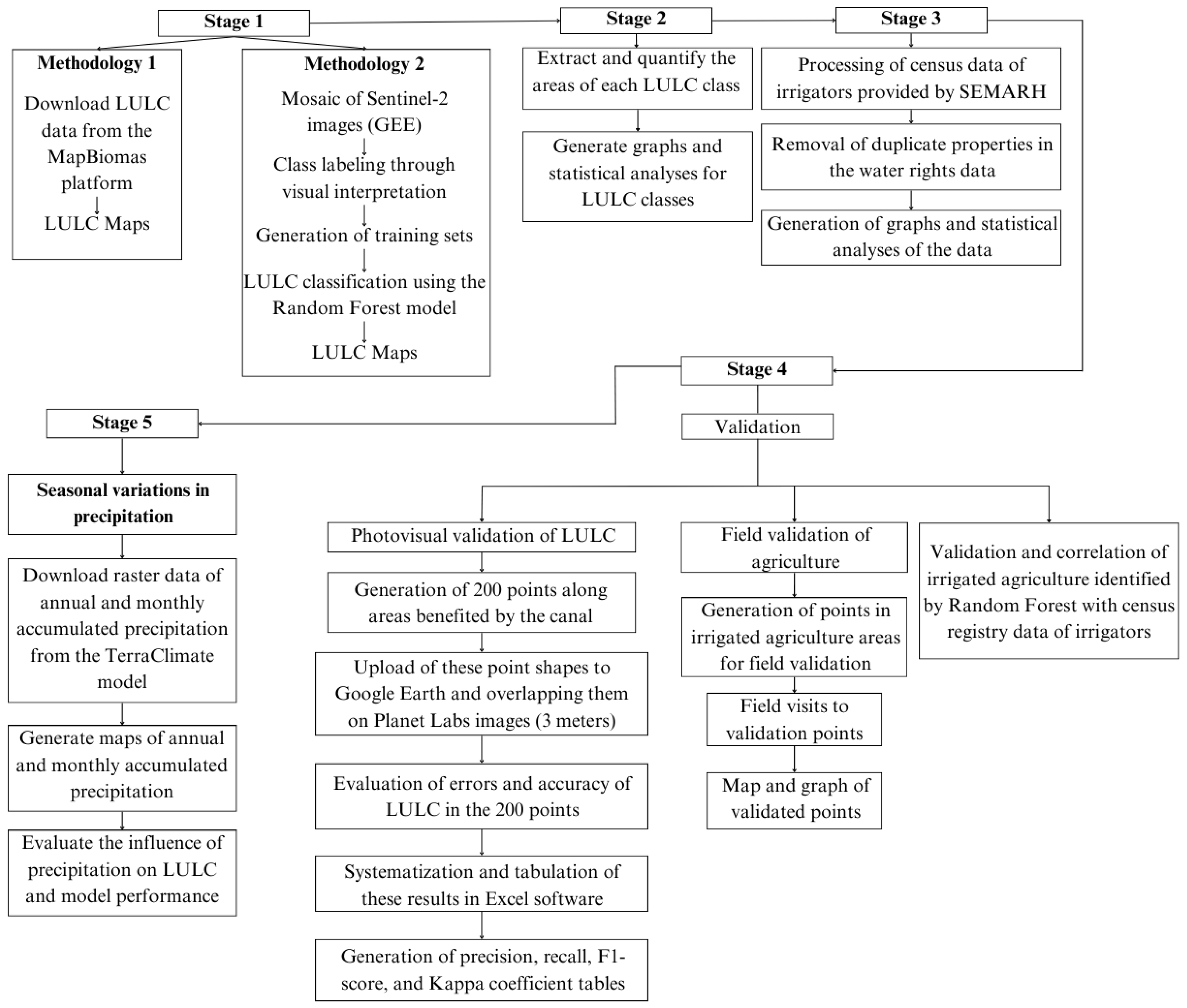
2.2. Methodological Flowchart

Figure 2 presents the methodological flowchart of this study, detailing the stages of data acquisition, processing, analysis, and validation of LULC data. Initially, MapBiomas data and Sentinel-2 images were used for supervised classification with the Random Forest algorithm. The classified areas were then quantified, validated, and statistically analyzed. Census data of irrigators provided by SEMARH were also processed, with duplicates removed and statistics generated. Subsequently, the results were validated through different approaches, including visual inspection, field validation with visits to agricultural areas, and correlation with census data. Finally, the influence of precipitation on LULC behavior was evaluated.

2.3. Obtaining the Shapefile of the Canal

A line shapefile was used to represent the entire length of the already-constructed section of the Canal do Sertão Alagoano, made available by the website “Alagoas em Dados e Informações” (https://dados.al.gov.br/; accessed on 19 March 2025). Subsequently, individual files were generated for each section, defined based on the canal’s route. The delimitation of the sections’ length was carried out based on official data published by the state government (https://parcerias.al.gov.br/projeto-canal-do-sertao/; accessed on 19 March 2025). Using the line shapefile as a reference, buffers with a 5 km radius were created on each side of the canal using the buffer tool in QGIS software (version 3.30). This approach aimed to delimit the canal’s influence zone.

2.4. Land Use and Land Cover (LULC) Classification Methodologies

2.4.1. LULC by MapBiomas

Based on data provided by the MapBiomas platform and processed in the GEE interface, LULC maps were generated for the regions benefited by the Canal do Sertão Alagoano. The LULC data from MapBiomas are derived from images of the Landsat-5/TM and Landsat-8/OLI sensors, with a spatial resolution of 30 m [16]. For this study, the MapBiomas Brasil Collection 8.0, level 4, was used, which offers 38 land use and occupation classes and subclasses. LULC maps were created for the period from 2016 to 2022, covering the classes water, forest, non-vegetated area, non-vegetative natural formation, natural pasture, agriculture, and mosaic of agriculture and pasture.
In addition to creating the maps, the areas corresponding to each class were quantified. For this, the spatial data from the raster files were extracted using Python (version 3.12.10), considering the four sections of the canal studied. Subsequently, the information was converted to XLSX format and organized into tables, allowing for the analysis of territorial transformations that occurred during the evaluated period.

2.4.2. LULC by Random Forest

The second stage of the study consisted of generating LULC maps using the Random Forest classification model, based on Sentinel-2 satellite image mosaics for the period from 2016 to 2022. Images from the months of October to December were selected, which fall within the dry season of the region (i.e., August to February), as determined by climate data on precipitation and air temperature from the INMET weather station located in the municipality of Pão de Açúcar. One of the reasons for choosing the dry period was the possibility of quantifying irrigated agriculture areas, as this practice stands out in semi-arid regions compared to other land uses [5]. The mosaics were created on the GEE platform (https://earthengine.google.com/; accessed on 16 September 2024) using a JavaScript script, with the Sentinel-2 image time series available in the GEE database.
To minimize cloud interference in the orbital images and identify irrigated agriculture areas, quality filters were applied to select images with the lowest percentage of cloud cover in the study area. For cloud removal in Sentinel-2 images, the QA60 band was used, which contains information about the presence of clouds and cirrus. Two masks were created from this band: one identifying cloud and another identifying cirrus. The mask was applied to remove pixels where these bits had a value of 1, preserving only pixels without atmospheric interference. As a result, mosaics were generated for the months of October to December each year, covering the entire length of the canal. The mosaic was generated using the red, green, blue, and NIR bands.
The supervised classification was performed using the Python programming language, integrating specialized libraries for geospatial data manipulation and machine learning, such as rasterio, geopandas, numpy, and scikit-learn [17]. The process began with reading the Sentinel-2 mosaics and the shapefiles containing the training geometries, which were previously generated in QGIS. The training mosaics were constructed based on the color, shape, and texture features from high-resolution Planet Labs images, with a spatial resolution of 3 m. Representative areas of each land use and land cover class were selected, identified by these observable patterns in the images. Within these areas, polygons were visually delineated according to those same features and classified into shapefiles containing an identifying column to differentiate the classes [5]. Table 1 shows the number of training polygons used for each class and year. As irrigated agriculture expanded over the years following the arrival of the Canal do Sertão, the number of polygons for this class also increased, as it became easier to visually identify these areas. In total, seven shapefiles were classified, one for each specific year.
The spectral pixels from the images were extracted based on the geometries of the training shapefiles, relating them to the defined classes: ‘Irrigated Agriculture’, ‘Non-vegetated area’, ‘Water bodies’, ‘Forest’, and ‘Natural pasture’. To train and evaluate the model, the train_test_split method from the scikit-learn library was used, where 70% of the samples were allocated for training, and the remaining 30% were used in the testing phase [16]. This division ensured the evaluation of the model’s accuracy with independent data from the learning process.
The Random Forest model was trained with 100 decision trees and a random seed to ensure the reproducibility of the results. During training, the classifier learned to differentiate the LULC classes based on the spectral values of the pixel bands. The classification was performed using the red, green, blue, and near-infrared (NIR) bands from Sentinel-2 images. After training, the classification was applied to the entire image, generating supervised LULC maps for each year. The resulting classifications were saved in raster files in TIFF format.

2.5. Accuracy Assessment of Random Forest and MapBiomas

An accuracy assessment was conducted to validate the LULC data obtained from the MapBiomas platform and the Random Forest model, using Google Earth software (version 7.3.6.10201) [3] and high-resolution (3 m) images from Planet Labs, accessed via the Planet Explorer plugin (version 2.3.4) in QGIS (version 3.40.6). Initially, a raster file containing 150 random points in the study area was generated using the “Random Points within Polygon” tool in QGIS. However, since these points were not significantly distributed over the agriculture and water body areas, which have a limited extent, 50 additional points were generated specifically within these classes. Considering that the canal’s influence area is limited and that irrigated agriculture areas are concentrated near its banks, a 2 km buffer was created for each side of the canal. The points representing the agriculture class were then generated within this buffer, ensuring better spatial representativeness of the data.
The identifiers (IDs) of the LULC classes associated with each point were extracted from the raster. This point file was imported into Google Earth and simultaneously overlaid onto monthly mosaics of images from Planet Labs in QGIS. Based on this integration, a visual analysis was conducted to check the agreement between the LULC classification and the characteristics observed in the high-resolution images, based on features such as color, shape, and texture, identifying correct and incorrect classifications of the models. The maps from 2021 and 2022 were used as they represent the most recent data and were close to the years of field visits. The results of this validation were organized and tabulated in Excel, enabling statistical analyses. To measure the accuracy of the classification, the Kappa coefficient was calculated, a statistical metric widely used to assess the degree of agreement between the LULC classifications and visual references, adjusting for agreements that might occur by chance [3]. The model’s performance was also evaluated through the metrics of accuracy, recall, and F1-score [17].
Precision measures the percentage of correct predictions among the samples that the model classified as belonging to a specific class. In other words, it indicates how many of the positive predictions made by the model were correct. It is calculated as shown in Equation (1):
Precision = TP TP + FP
where TP (true positives) represents the samples correctly classified as belonging to the class, and FP (false positives) corresponds to the samples that were incorrectly classified as belonging to the class [17].
Recall measures the percentage of correct predictions among all the samples that actually belong to a specific class. In other words, it indicates the model’s ability to correctly identify positive examples of a particular class. It is calculated as shown in Equation (2):
Recall = TP TP + FN
where TP (true positives) represents the samples correctly classified as belonging to the class, and FN (false negatives) refers to the samples that belonged to the class but were incorrectly classified as another category [17]. The F1 score is the harmonic mean between precision and recall, and it is used to balance both metrics, especially in cases of imbalanced data.

2.6. Generation of the Normalized Difference Vegetation Index (NDVI)

NDVI calculations were performed on the GEE platform for the dry season, covering the period from October to December, independently for each year and section of the canal analyzed. The NDVI calculation for the canal sections was based on the multispectral surface reflectance bands, as expressed in Equation (3):
NDVI = ( NIR RED ) ( NIR + RED )
where NIR and RED are the near-infrared and red bands, respectively, from Sentinel-2.
The NDVI raster images were extracted and processed using QGIS software, version 3.30. Based on these images, NDVI maps were generated for Sections I–IV for the period from 2016 to 2022. These maps were used to compare with LULC data, with the expectation that forest and irrigated agriculture areas would exhibit higher NDVI values than other classes. This served as a way to assess the agreement between the maps generated by the Random Forest model and the NDVI [8].

2.7. Analysis of Water Abstraction Points and Water Grants in the Canal Areas

The Secretariat of the Environment and Water Resources (SEMARH) of the state government of Alagoas provided a database of registered irrigators authorized to use water from the Canal do Sertão Alagoano. The data provided by SEMARH included the year of registration, the size of the irrigated area, and the location of the water abstraction point, among other information. For this study, the location of the abstraction points and the size of the irrigated area were used to perform correlation analyses between the registered irrigators’ areas and the irrigated agriculture area identified by the Random Forest model.
This registration by SEMARH was carried out in the municipalities already benefiting from the Canal do Sertão Alagoano, namely Delmiro Gouveia, Pariconha, Inhapi, Água Branca, Olho D’Água do Casado, Senador Rui Palmeira, and São José da Tapera. Several campaigns were conducted to encourage farmers to register at the various available locations and to regularize their water abstraction from the canal. In addition to receiving the water use permits, farmers participated in technical training on the proper use of water and received technical assistance. The process was concluded with the integration of all data into a comprehensive table to support the Technical Diagnostic Report of the Sertão Adductor Canal.
The data provided for this study were processed to remove duplicate information. Cases where the same producer had more than one record for the same location and/or the same irrigated area, even in different years, were excluded. To streamline this process, a Python script was developed to scan the Excel spreadsheet and eliminate duplicate information related to landowner names, latitudes, and longitudes.
The total irrigated agriculture area for each year, according to SEMARH data, was calculated and recorded in a spreadsheet. In the same spreadsheet, the total irrigated agriculture area estimated by the Random Forest model was also included. These data were used for the correlation analysis between the total estimated irrigated area and the census data provided by SEMARH.
A second correlation analysis was conducted between the area estimated by the Random Forest model and the SEMARH data, considering smaller sections, with a 2 km extension on each side of the Canal do Sertão Alagoano margins and horizontal intervals of 1 km. This approach was adopted after verifying that the canal’s area of influence is limited and that irrigated agriculture is primarily concentrated in its vicinity.
A 2 km buffer was generated on each side of the canal margin and saved in shapefile format. This shapefile was divided into horizontal segments at 1 km intervals. Due to the numerous curves of the canal, the segments exhibited significant variations in size, as the division was performed using straight vertical lines regardless of the canal’s direction. To mitigate this issue and ensure a fair assessment of the areas, the correlation analysis was conducted only in a straighter section of the canal, in the horizontal direction, resulting in a total of 14 segments within the selected area. The correlation considered the irrigated area in each segment, based on the SEMARH census records, and the irrigated area identified by the Random Forest model. All procedures in this analysis, including reading SEMARH data (coordinates of water intake points and irrigated area associated with each point), shapefile segmentation, and statistical correlation analyses, were performed using the Python programming language.

2.8. Field Visits for Agriculture Validation

In the QGIS software, sample points were generated, and the geographic coordinates of these points were used for in situ visits to validate the accuracy of the Random Forest model in identifying areas designated for irrigated agriculture. Some of the points were predefined based on the LULC classification of the model, focusing on regions classified as irrigated agriculture. The remaining points were identified directly in the field, taking advantage of opportunities to contact local producers, which allowed access to properties with agricultural production, totaling 33 points for Random Forest validation. Additionally, 12 more points were collected, this time in rainfed agriculture areas, to validate MapBiomas, with the goal of evaluating the model’s ability to identify this LULC class in the study area.

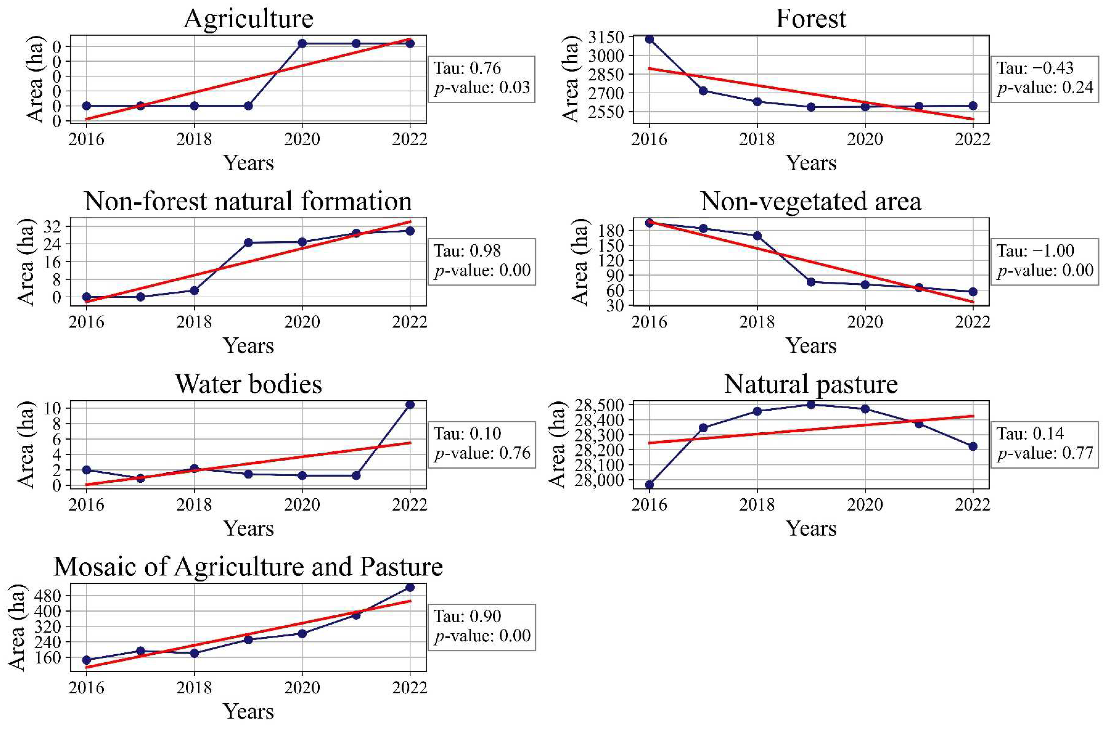
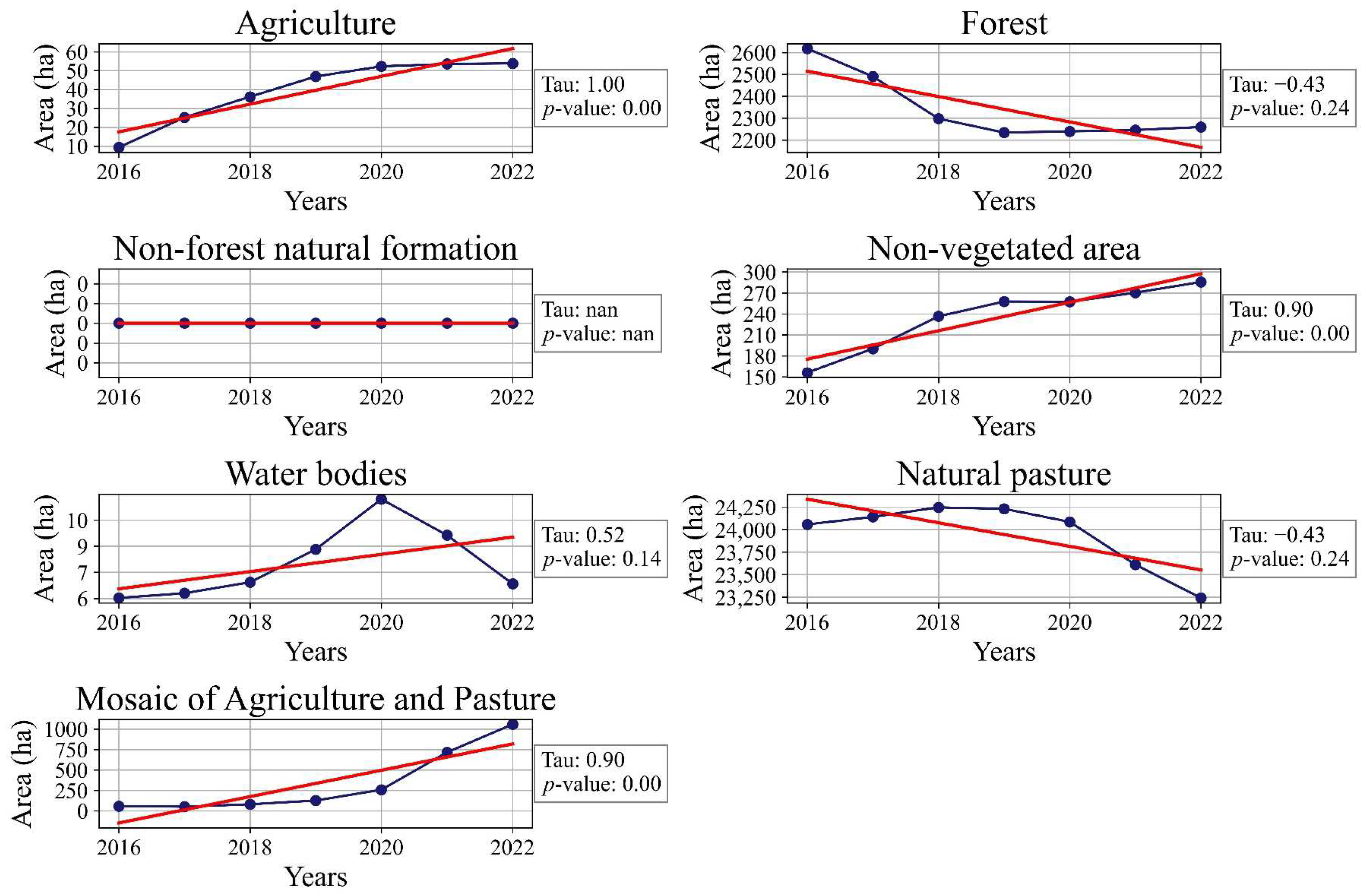
2.9. Temporal Analysis of Land Use and Land Cover Classes

The areas of each LULC class were quantified from the maps generated by MapBiomas and the Random Forest model. The values were extracted directly from the rasters and organized into Excel spreadsheets. For each LULC class, line graphs were created to represent the temporal variation, accompanied by a trend line derived from linear regression analysis. Additionally, the Mann–Kendall statistical test was applied to assess the significance of the observed trends, using the correlation coefficients τ and the p-value.

2.10. Seasonal Variation in Precipitation

To assess the influence of precipitation on land use and land cover, data from the Terraclimate climate model were used. Specifically, precipitation data for the state of Alagoas were obtained, including both annual totals and monthly totals for October, November, and December, corresponding to the land use and land cover maps generated by the Random Forest algorithm. The data, provided in raster format with a spatial resolution of 4 km, were processed in QGIS to create precipitation maps for the period from 2016 to 2022. From these maps, it was possible to analyze the vegetation behavior during wet and dry years, allowing a comparison between different climatic patterns.

3. Results

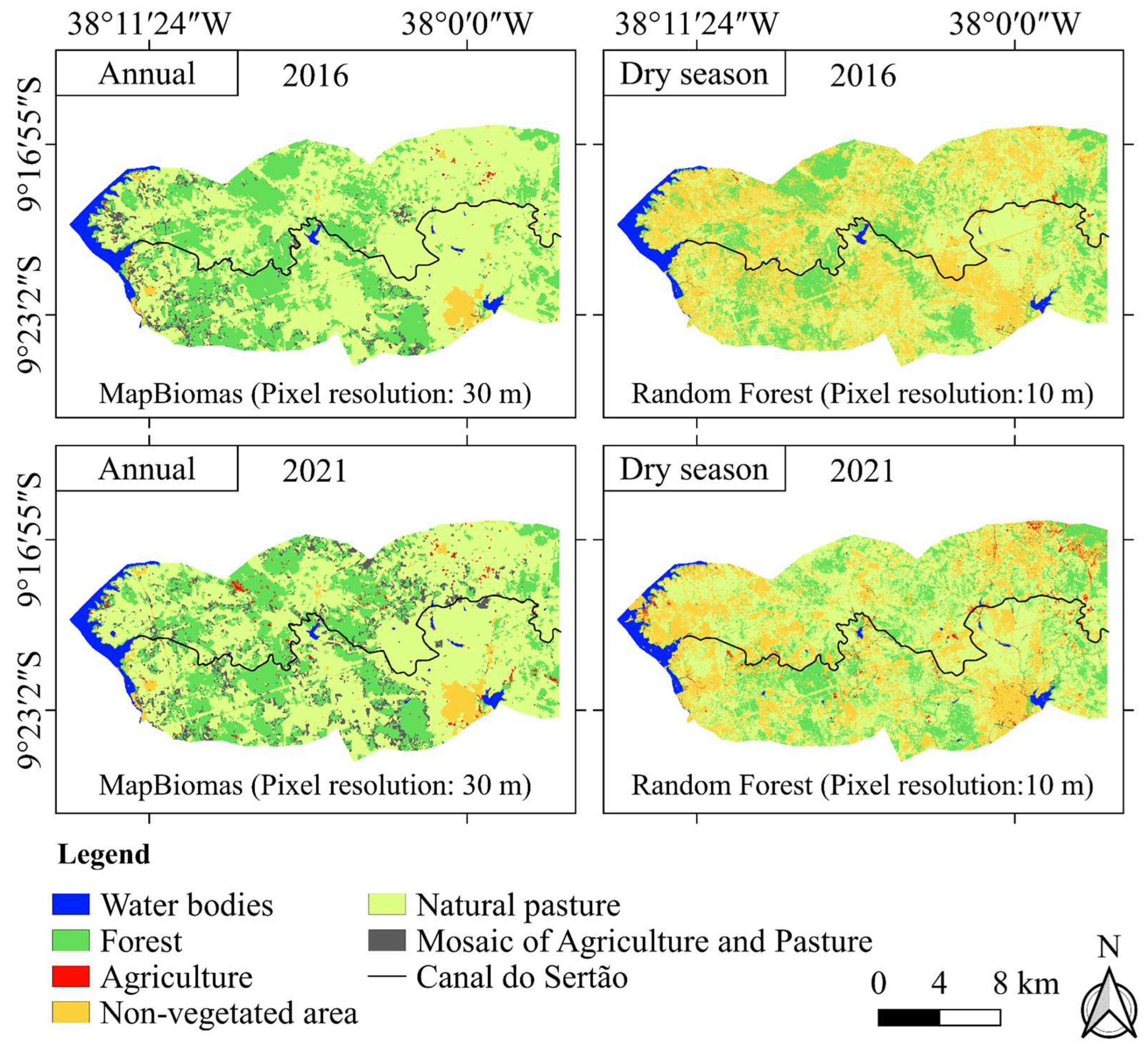
3.1. Validation of Land Use and Land Cover Classification Models

The overall accuracy of LULC mapping by MapBiomas, based on 200 validation points, achieved a Kappa coefficient of 0.74 (Table 2). When analyzing the categories individually, the land use and land cover classes showed an accuracy above 90%, except for the agriculture category. The accuracy for the agriculture class is low (41%), indicating that when the model predicted agriculture, only 41% of the predictions were actually correct. This may be related to the fact that agriculture in the region consists predominantly of small areas, while MapBiomas operates with a 30 m resolution and annual pixel averages. Therefore, seasonal dynamics and the rapid landscape changes in regions such as the Sertão pose a challenge for mapping accuracy. Agriculture in the Sertão is an activity that develops over a few months in small-sized areas, making its precise identification difficult among the sensor’s pixels. Recall measures the proportion of actual positive cases that the model successfully identified. Thus, of all the samples that truly belong to the agriculture category, the model correctly identified 89%. The F1 score is the harmonic mean between precision and recall metrics. In this case, the agriculture and forest classes presented lower F1 score values compared to the other classes.
The Random Forest model achieved a Kappa value of 0.82, based on 200 validation points (Table 3). When analyzing the classes individually, Random Forest showed an accuracy of 65% for agriculture and above 85% for the other classes. Recall indicated that of all samples that truly belong to the agriculture category, the model correctly identified 100%. The F1 score for agriculture was 79%, higher than the 56% obtained by MapBiomas. This difference can be explained by several factors, the main one being that the Random Forest model was specifically calibrated for the study region. Additionally, Random Forest focused on the region’s dry season, during which agriculture stands out significantly from natural vegetation, as it is almost exclusively irrigated.

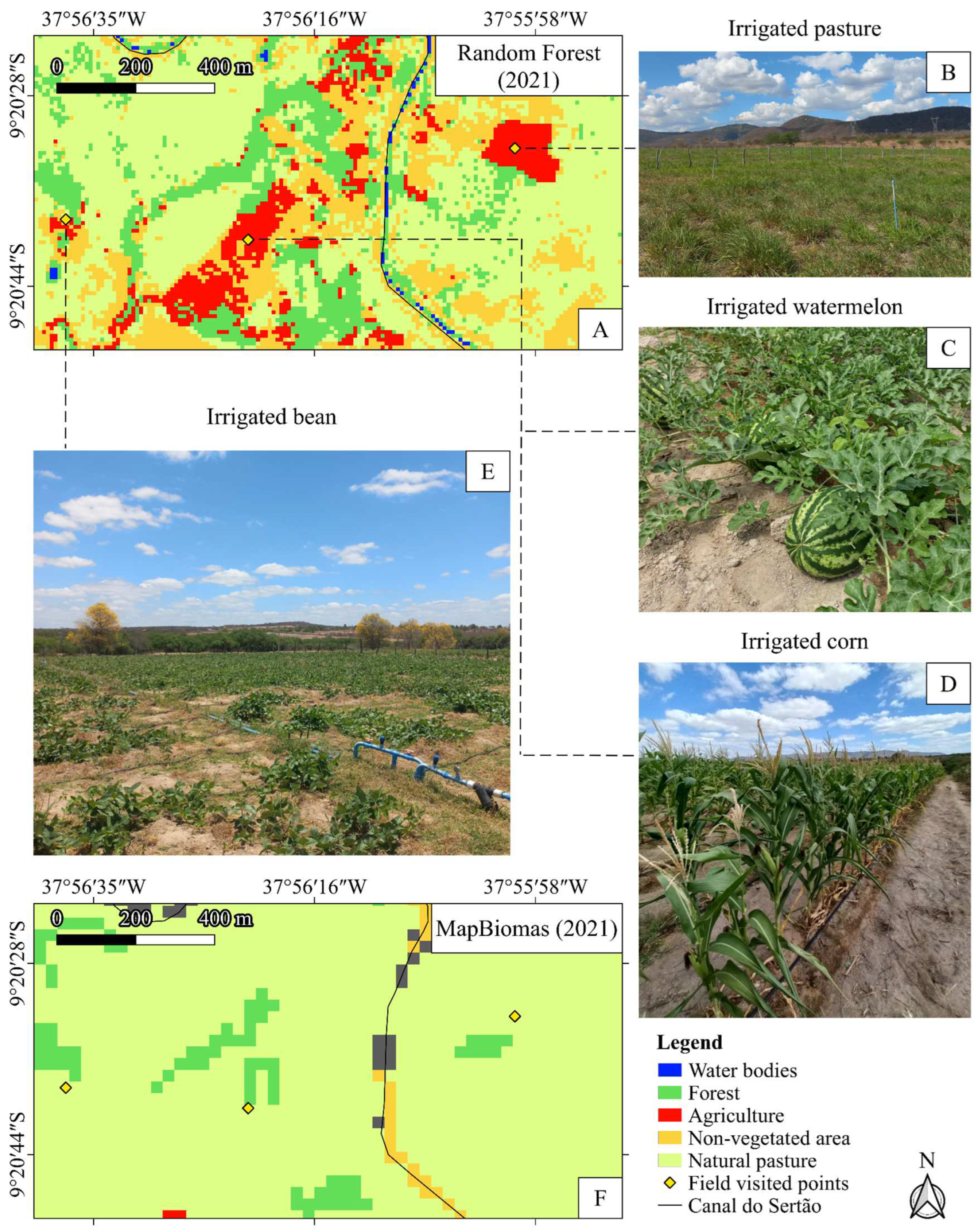
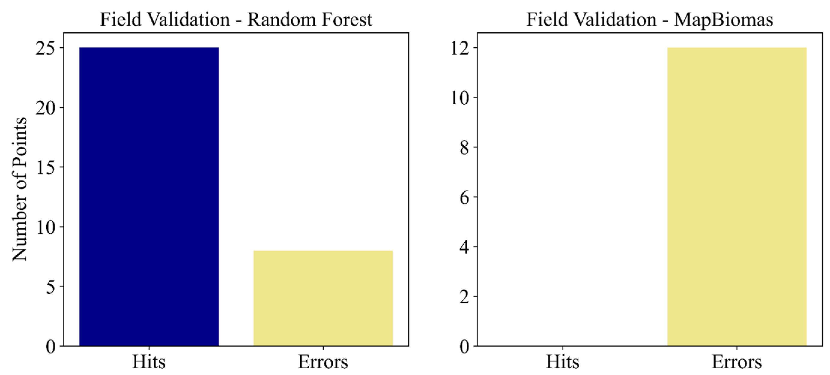
3.2. On-Site Validation of the Accuracy of the Random Forest and MapBiomas Models for Agriculture Classification

Field visits were conducted to validate the model’s accuracy in identifying irrigated agriculture areas. Figure 3 shows an area near the canal in the municipality of Água Branca, where, at the central point, crops such as watermelon, corn, pumpkin, and other irrigated cultures were found, all using water from the Canal do Sertão Alagoano. The point to the east of the map corresponds to a pasture area irrigated by sprinklers, while the point to the west represents a property cultivating beans, vegetables, cassava, and corn, where the property owners emphasized their intention to expand the irrigated area in the coming years. It was not possible to access all nearby properties, as some are private, and there was no contact with the owners. However, while surveying the region, it was possible to observe similarities between the maps generated by the Random Forest model and the local reality. On the other hand, when analyzing the LULC classification from MapBiomas for the same location and year, it was observed that agriculture was not identified. Since these are irrigated agriculture areas, they were expected to be present throughout most of the year and, consequently, to be detected by MapBiomas, which operates with the annual average of the pixel. However, MapBiomas failed to identify these areas in Figure 3.
A total of 33 points were visited in selected areas for the validation of the Random Forest model. Some of these points were predefined based on the model’s LULC classification, focusing on regions classified as irrigated agriculture. The remaining points were identified directly in the field, taking advantage of opportunities to engage with local farmers who allowed access to their properties where agricultural production was observed. The model demonstrated good performance, correctly classifying 25 points compared to 8 points where errors were detected (Figure 4). Additionally, during field visits to rainfed agriculture areas, 12 additional points were collected for MapBiomas validation. However, the model failed to identify these agricultural areas among the visited points. This is partly due to the seasonal nature of agriculture in the region, which is concentrated during the rainy season—an aspect that makes detection challenging for models that rely on the annual pixel average, such as MapBiomas.
When evaluating the LULC maps generated by the Random Forest model alongside field visits, it was observed that irrigated agriculture areas are located near the canal margins. As the distance from the canal increases, some of the agriculture areas identified by the model contain errors in a lowland region, where natural pasture vegetation remains green even during the dry season due to soil moisture accumulation in this area (Figure 5). This misclassification by the model occurred because the spectral responses of this vegetation are similar to those of irrigated agriculture areas.

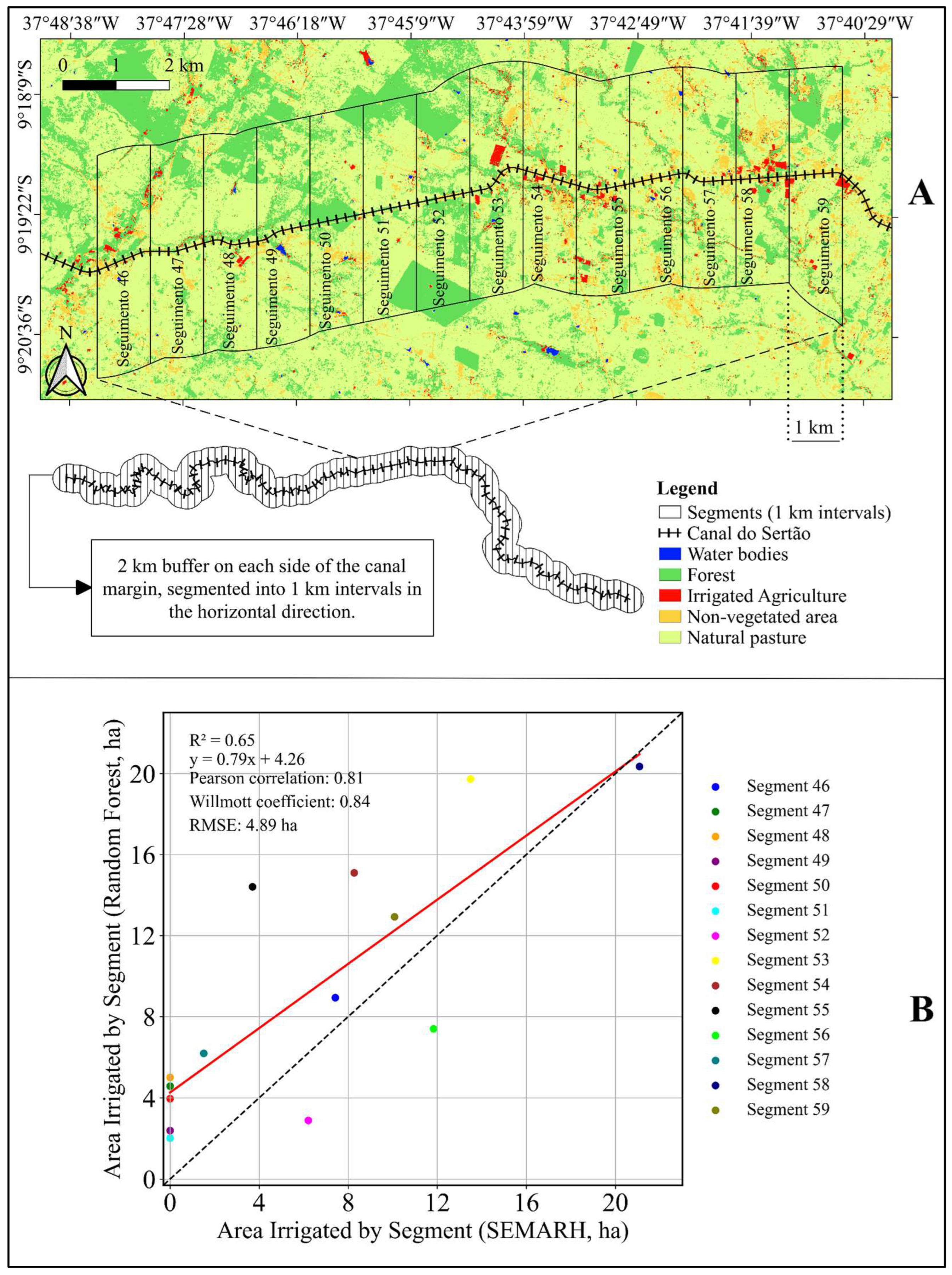
3.3. Validation and Correlation Between Estimated Data (Random Forest) and Irrigation Census Registration Data (SEMARH)

The actual irrigated agriculture data provided by SEMARH and those obtained from the Random Forest model showed a high positive correlation (r = 0.85) (Figure 6). These results indicate a good agreement between the observed data and those estimated by the model. The Root Mean Squared Error (RMSE) revealed that the average deviation between the observed and predicted values was 360.76 ha, highlighting a tendency of the model to overestimate the irrigated agriculture areas, with four points above the 1:1 line. It is important to note that the actual irrigated agriculture data provided by SEMARH may not represent the full extent of irrigated areas, as not all farmers who use water from the Canal do Sertão Alagoano for irrigation are necessarily registered or legalized.
In Figure 7A, the map shows the Canal do Sertão Alagoano with a 2 km buffer on each bank, divided into segments with 1 km intervals. Each segment is numbered (from 46 to 59) and contains the LULC classes for the year 2021. In the drawing below the map, it can be seen that the full path of the canal has several curves. However, the segments are divided by straight vertical lines, regardless of the canal’s curves. This can lead to variations in the sizes of the segments and, in some cases, prevent the irrigated areas from being correctly framed, as these areas follow the winding course of the canal. For this reason, the correlation analysis was carried out only in segments 46 to 59, which represent the most homogeneous areas of the canal. Figure 7B shows the scatter plot, comparing the irrigated area identified by the Random Forest model with the census data of irrigated areas from SEMARH within each segment. The results indicate a strong positive correlation (r = 0.81) between the irrigated areas estimated by the model and the census data, with a coefficient of determination (R2) of 0.65, demonstrating that the model explained 65% of the observed variation. This R2 value can be explained by the possibility that not all irrigators are registered, as registration was carried out through campaigns where irrigators needed to visit registration points. Additionally, there is the limitation of the model in lowland areas, causing spectral confusion. It is observed that when SEMARH recorded zero irrigated areas in certain segments, the model also identified few irrigated areas in the same segments (from 47 to 51).

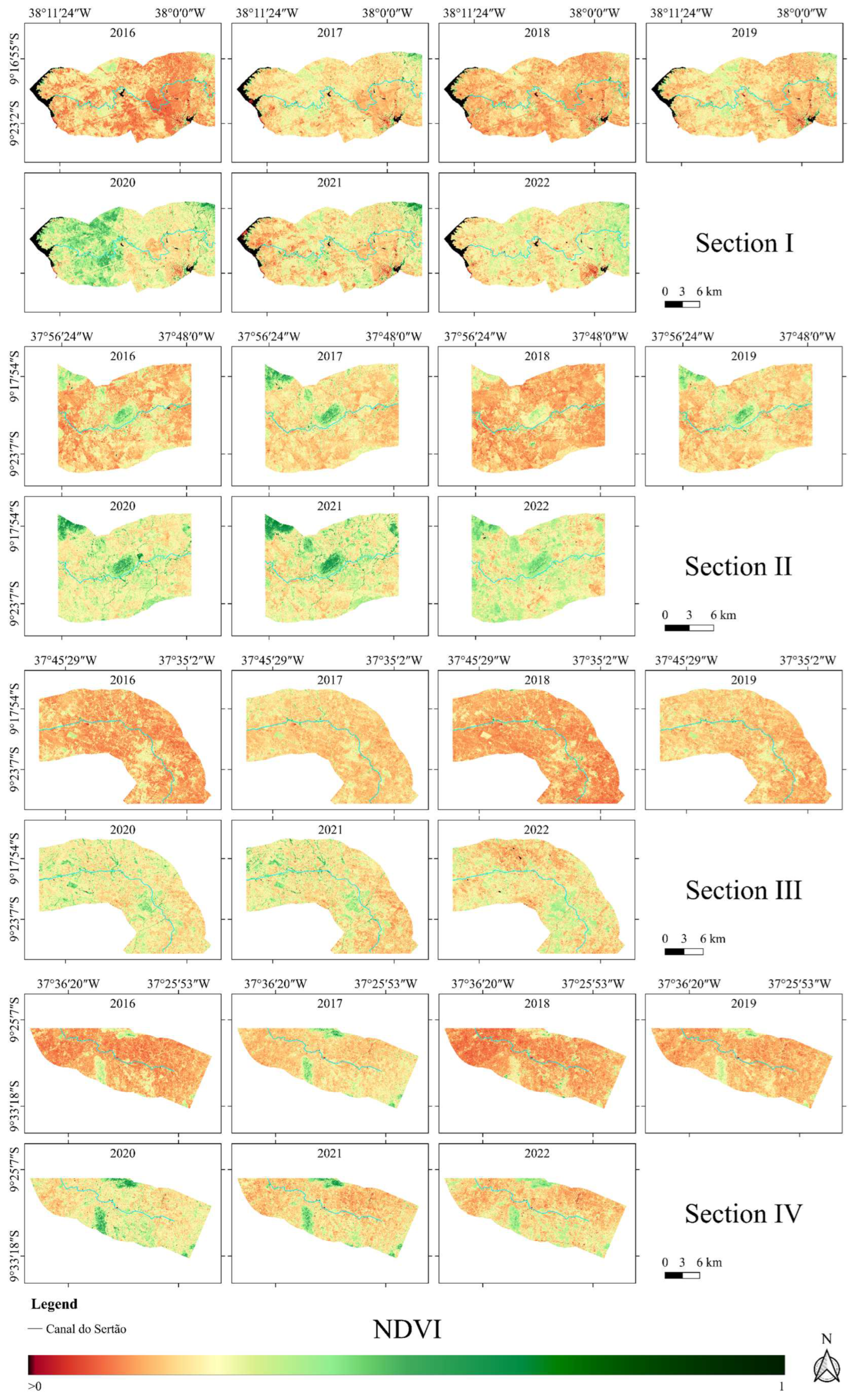
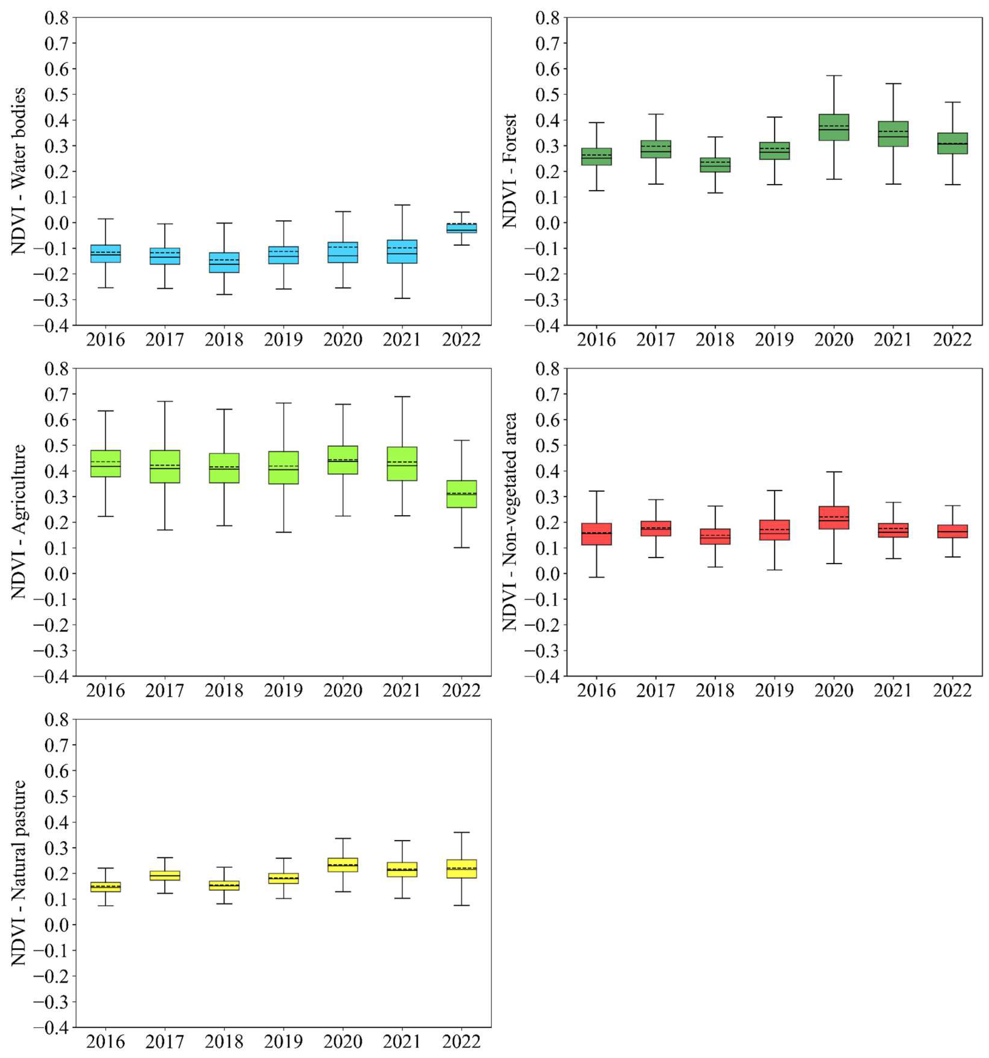
3.4. Normalized Difference Vegetation Index (NDVI)

When evaluating the Normalized Difference Vegetation Index (NDVI), higher values can be observed in areas classified as forest. Irrigated agricultural areas also showed higher NDVI values compared to other classes. Non-vegetated areas exhibited lower NDVI values, evident through the redder color in areas where this class is present. Water bodies presented a color tending toward black, with part of the São Francisco River in the western section of the maps in Section I being easily identifiable, where water from the canal is captured. In wetter years such as 2020 and 2022, the NDVI shows a visible increase (Figure 8). In drier years, the red color intensifies, indicating a decrease in NDVI due to the increase in exposed soil and the loss of vegetation quality.
The boxplot graphs illustrate the typical behavior of each land use and land cover class (Figure 9). The observed values align with expectations: water bodies show an NDVI near or below 0, due to low reflectance in the near-infrared (NIR) range. In forest areas, the average NDVI ranges from 0.23 to 0.37, which could be consistent with the characteristics of Caatinga vegetation, known for its sparse cover and low density during the dry season. Irrigated agriculture shows a slightly higher average NDVI (0.31–0.44), with quartiles ranging from 0.25 to 0.49, accompanied by high variability, reflecting the diversity in agricultural practices and crop conditions. Non-vegetated areas, such as exposed soil or urbanized zones, show an average NDVI below 0.23. Natural pasture areas exhibit an average NDVI between 0.14 and 0.23, which could be due to the low density and quality of pastures in Caatinga regions during the dry season.

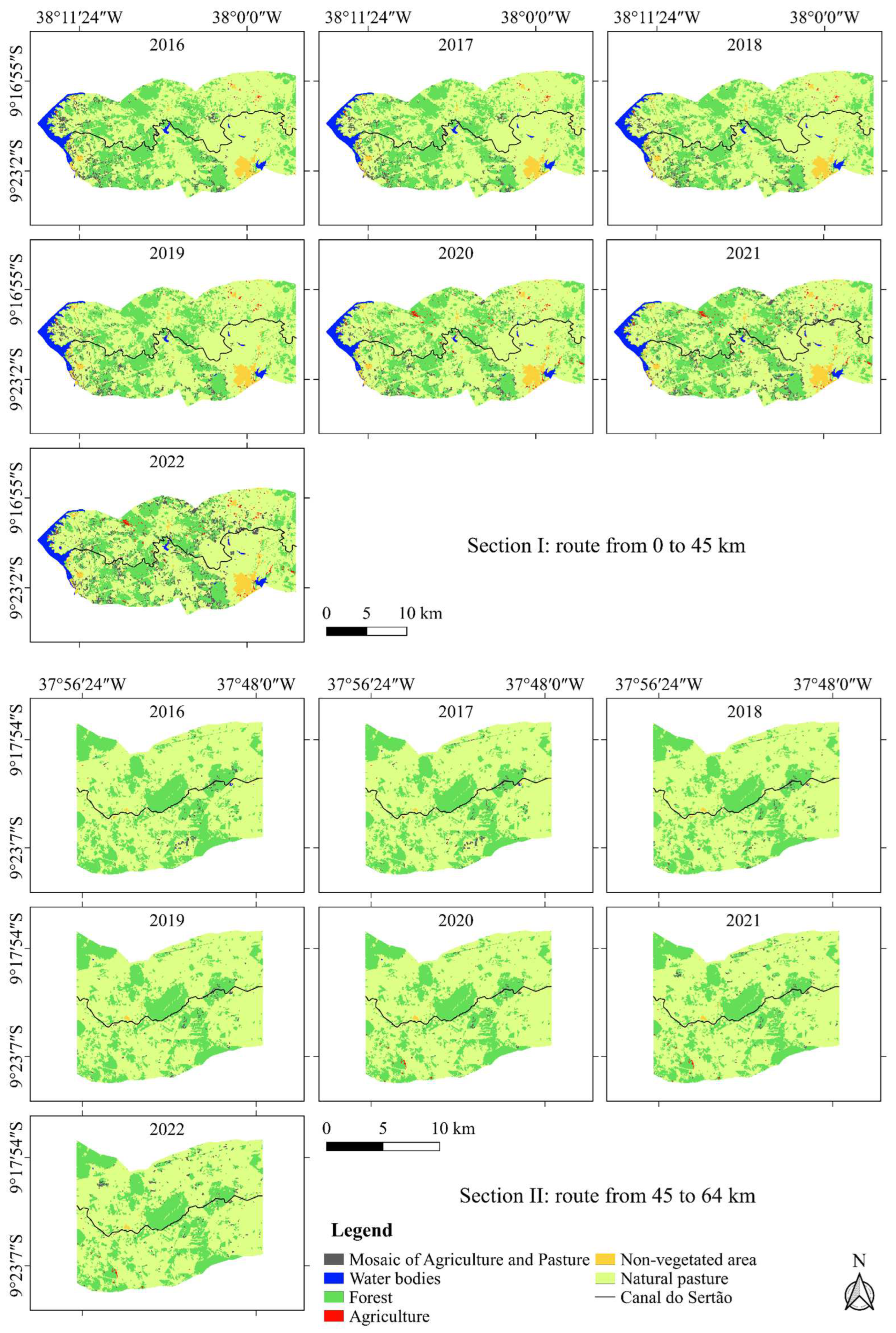
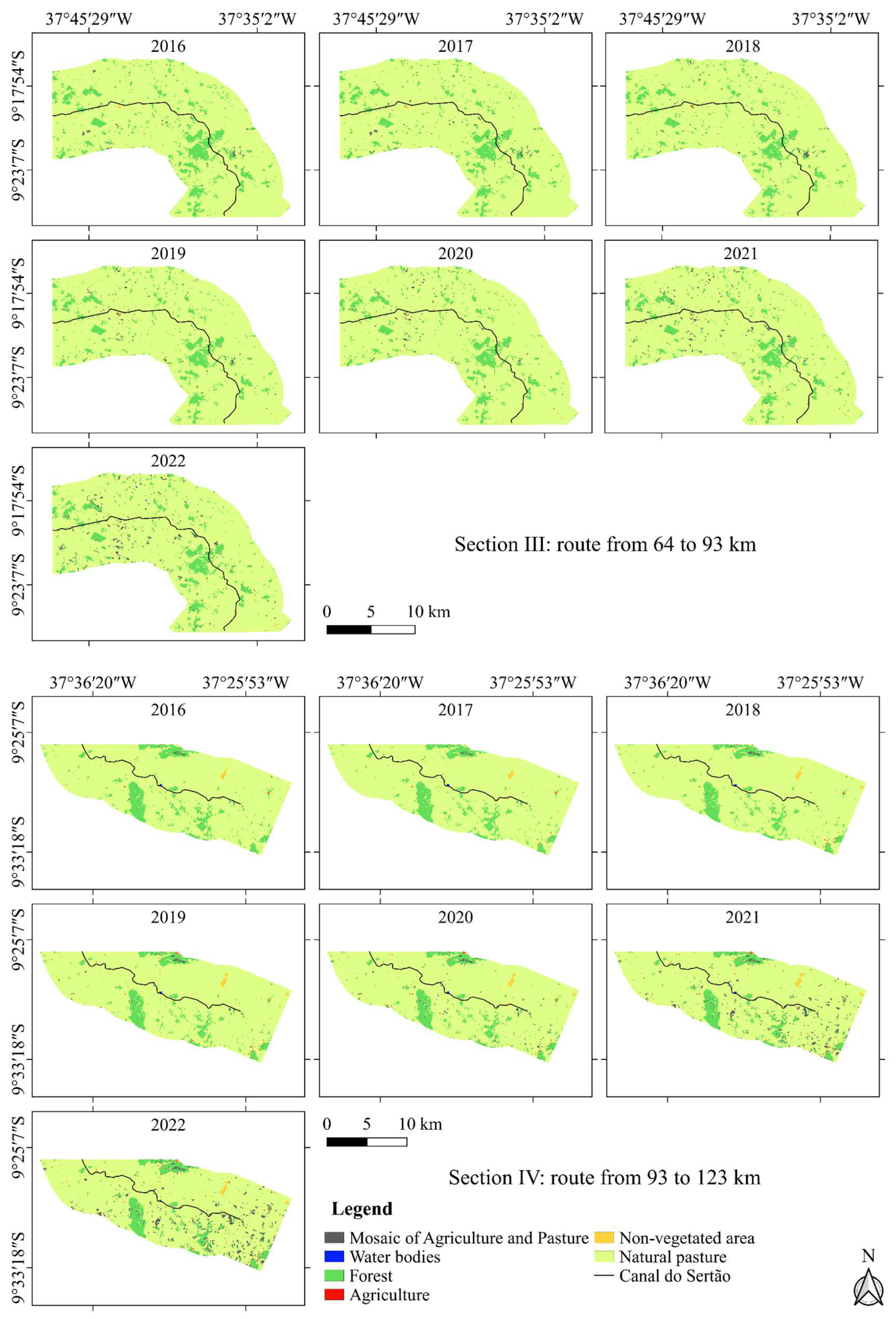
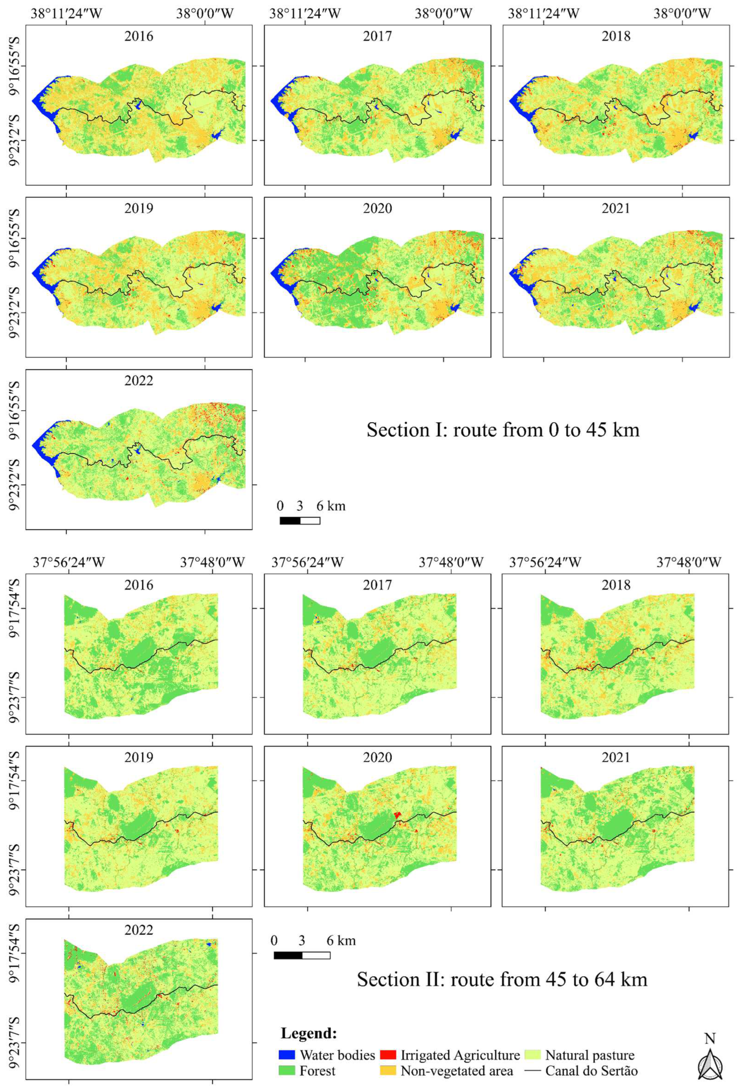
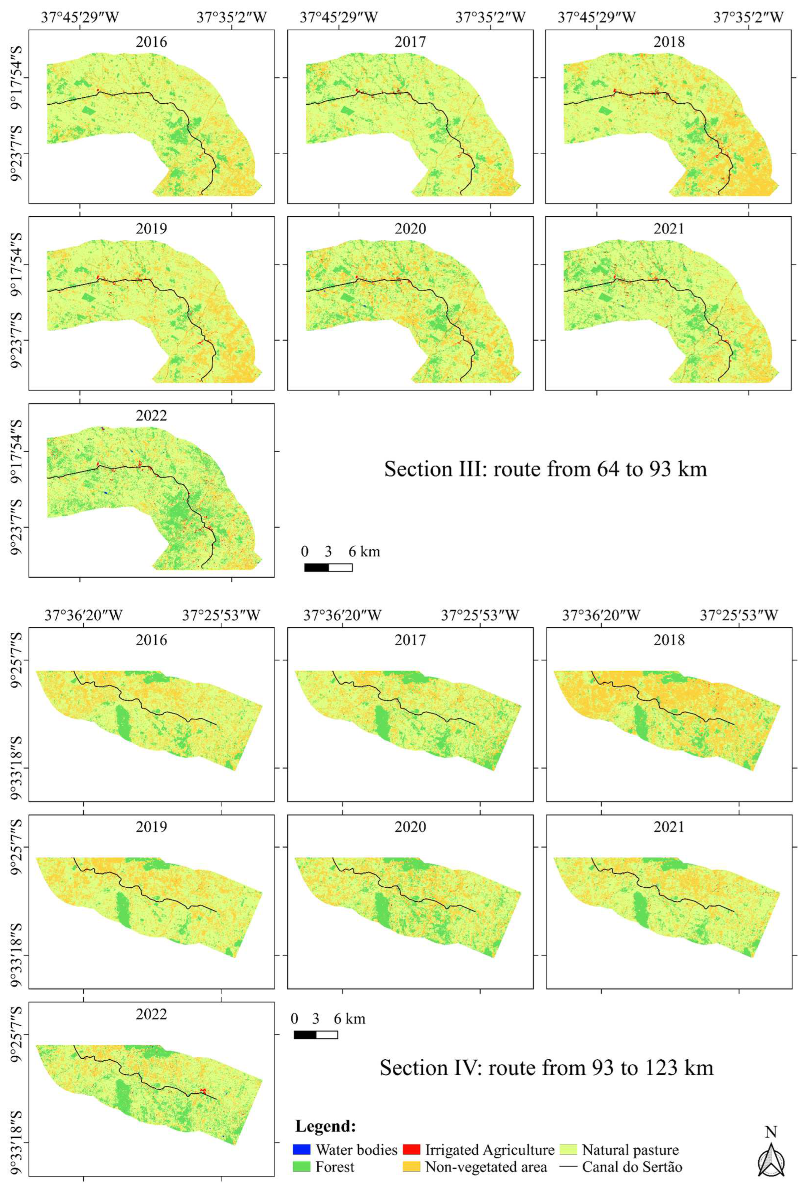
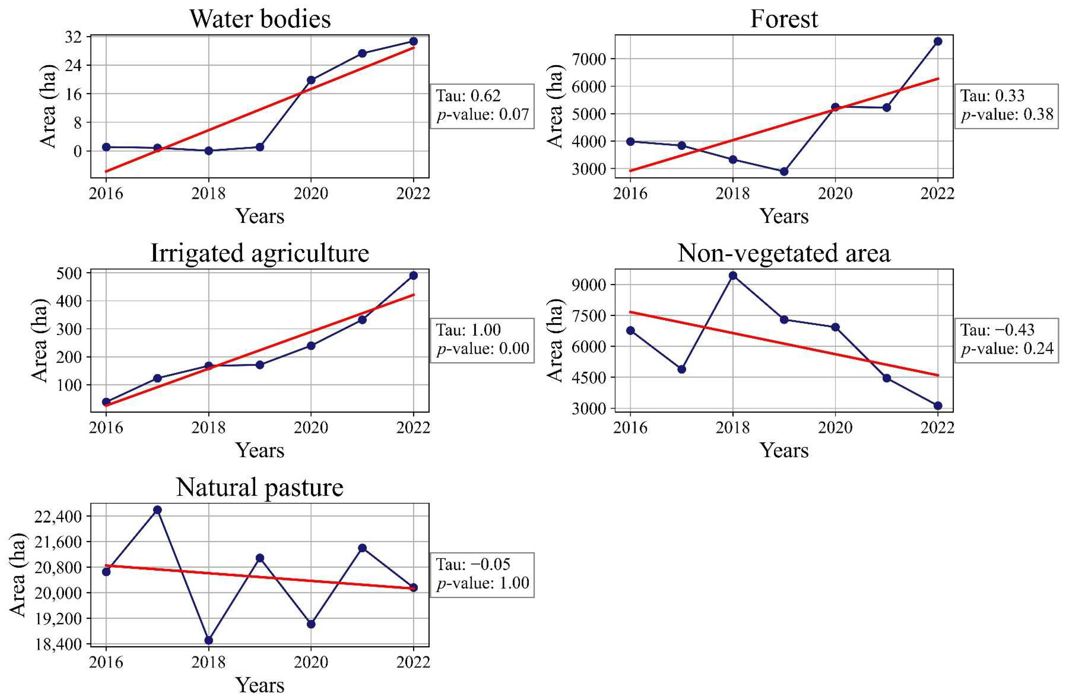
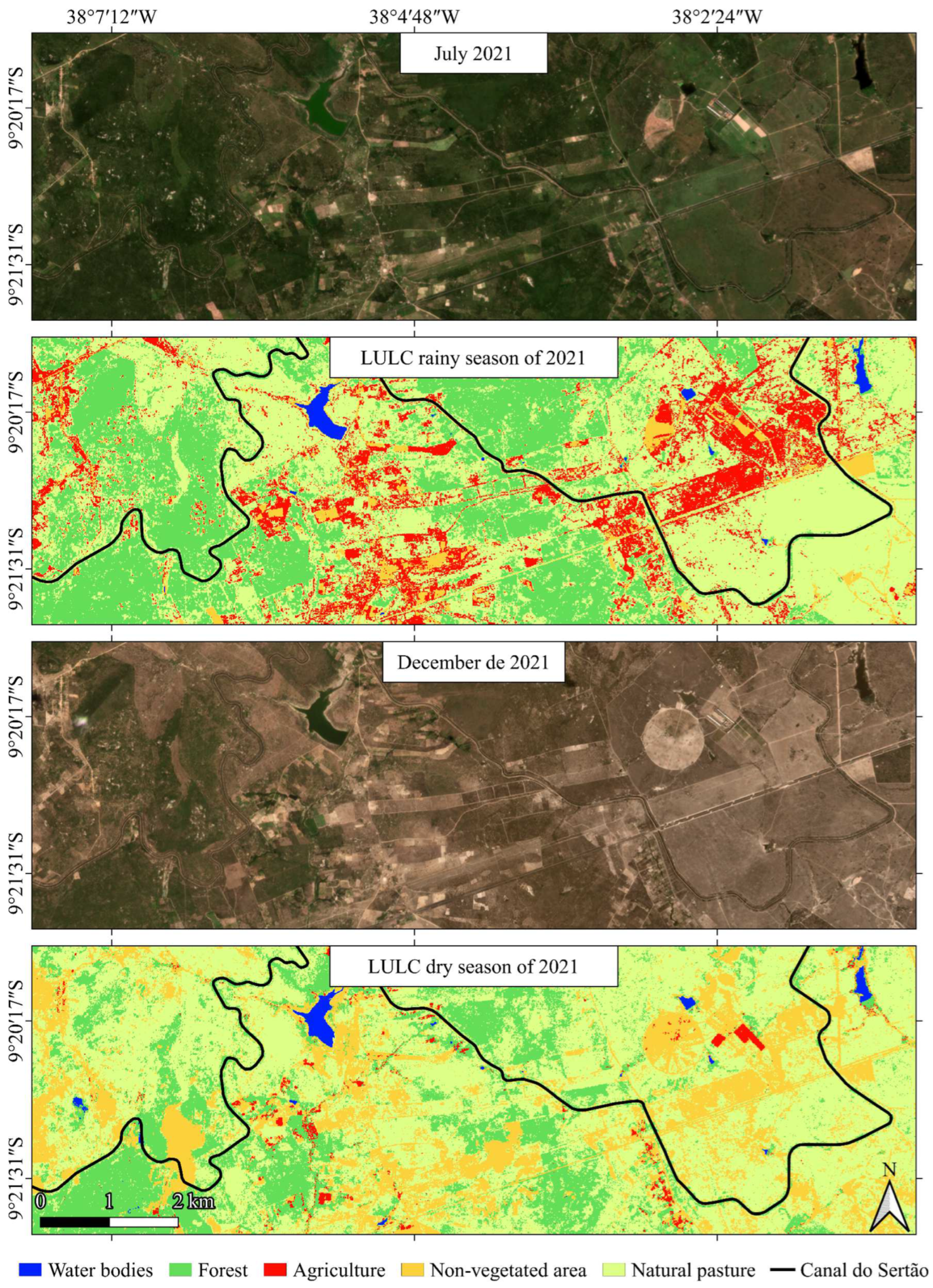
3.5. Land Use and Land Cover (LULC) Analysis (MapBiomas)

Section I of the Canal do Sertão Alagoano exhibited the most noticeable land use and land cover (LULC) change (Figure 10). At the eastern end of the map, a small part of the São Francisco River can be seen, where the system that captures water and transports it to the canal’s starting point is located, continuing its path by gravity. The expansion of the “Mosaic of Agriculture and Pasture” class is noticeable, which represents areas of agricultural use where it was not possible to distinguish between pasture and agriculture. The areas recognized as agricultural are scarce and small in size. Pasture is the predominant class throughout the entire evaluated period and represents a natural vegetation of the Caatinga, with herbaceous and/or shrub plants. Section II is the shortest section of the canal, at only 19 km, where the dominance of forest and pasture classes is also observed (Figure 10). It is noted that agriculture remains very limited in area. The “Mosaic of Agriculture and Pasture” class, which may include some agriculture, occupies a larger area than the areas exclusively classified as agriculture in these sections, although it is still small compared to other land uses.
From 2016 to 2022, a series of changes in the distribution of LULC in this section of the canal were observed, with the “Agriculture” class showing growth. Overall, this class exhibited significant growth (p < 0.05) over the studied years, with a τ value of 0.81. In 2016, an initial area of 67 ha was observed, with subsequent stability. Then, starting in 2017, areas occupied by agriculture showed an increase, reaching their peak in 2021, with a total area of 293 ha (Figure 11). The “Natural pasture” area showed an initial increase followed by a decrease, reaching 22,574 ha in 2022. The “Mosaic of Agriculture and Pasture” class was larger than agriculture, with 2861.64 ha in 2022. However, since this category includes areas where it was not possible to distinguish between agriculture and pasture but represents agricultural land uses, it is possible that it includes areas that should be classified as agriculture. This occurs due to the limitations of the MapBiomas model in precisely defining these areas. The “Mosaic of Agriculture and Pasture” and “Natural pasture” did not show a significant trend (p > 0.05).
When analyzing Section II of the Canal do Sertão Alagoano, it was observed that the “Agriculture” class showed an initial stability, reaching its lowest value in 2018, with 0.6 ha. Starting in 2020, the area began to expand, reaching 20 ha in 2022 (Figure 12). This agricultural area is quite small and likely does not reflect the actual value of the region, indicating an underestimation by the MapBiomas model. The classes that did not show statistically significant trends according to the Mann–Kendall test (p > 0.05) were “Agriculture” (τ = 0.55), “Forest” (τ = −0.62), “Non-vegetated area” (τ = −0.52), “Natural pasture” (τ = 0.43), and “Mosaic of Agriculture and Pasture” (τ = 0.14).
In Section III, it is possible to observe a predominance of the pasture class, representing almost 90% of the entire area. The agricultural area is almost imperceptible, with Section II having the smallest agricultural area compared to the other sections (Figure 13). The “Mosaic of Agriculture and Pasture” class, as previously mentioned, may encompass agricultural areas and is slightly more prominent, although it is still characterized by small areas. In this section, the canal curves to the south of the map, and its length in this section is 29 km. Section IV of the canal was the last to be constructed and delivered, and it has a larger annual agricultural area than Sections II and III, according to the MapBiomas data (Figure 13). The LULC characteristics in this section are similar to those already presented, with a predominance of the pasture class and two regions of denser forest. Agriculture is almost imperceptible. The mosaic of agriculture and pasture class shows a noticeable increase when comparing the initial map and the 2022 map, where this increase in agriculture in 2022 is likely related to the higher precipitation that occurred in that year throughout the state of Alagoas.
During the period from 2016 to 2022, Section III revealed patterns similar to those previously presented (Figure 14). Agriculture showed a significant growth trend (p < 0.05). However, this class represents a very small area, with less than 1 ha. This indicates that MapBiomas was unable to classify the agriculture in the region, and part of this agriculture should be within the “Mosaic of Agriculture and Pasture” class, where the model could not define which of these land uses the evaluated pixel actually belonged to. The “Mosaic of Agriculture and Pasture” class started with 145 ha in 2016 and then showed almost constant growth until 2022, totaling 522 ha, with this growth being significant (p < 0.05).
Between 2016 and 2022, significant changes occurred in the LULC distribution in Section IV (Figure 15). The “Agriculture” class showed initial growth from 2016 to 2020, followed by stability, reaching 54 ha in 2022. Agriculture experienced significant growth (p < 0.05) and occupies a larger area than Section III, although still small. The “Natural Pasture” class remained relatively stable until 2020, when it decreased, reaching 23,241 ha in 2022. According to the Mann–Kendall statistical analysis, this class did not show a significant trend (p > 0.05). The “Mosaic of Agriculture and Pasture” class showed a significant growth trend (p < 0.05), covering an area larger than agriculture, reaching 1057.5 ha in 2022.
When comparing the LULC maps from MapBiomas with those generated by the Random Forest model, significant differences are observed (Figure 16). This is mainly due to differences in spatial and temporal resolution between MapBiomas and Random Forest, in addition to the training samples, as Random Forest was exclusively trained for the region of interest. The Random Forest model used only images from the months of October to December, corresponding to part of the dry season in the study region. This period was chosen to identify areas of irrigated agriculture, since rainfed agriculture is nearly nonexistent during this time of the year due to the lack of water and the extremely dry and hot climate. This is also reflected in the large presence of non-vegetated areas in the maps generated by Random Forest, as during this time of year, the Caatinga vegetation in northeastern Brazil tends to lose all its leaves, transforming the landscape in the Alagoas hinterland.

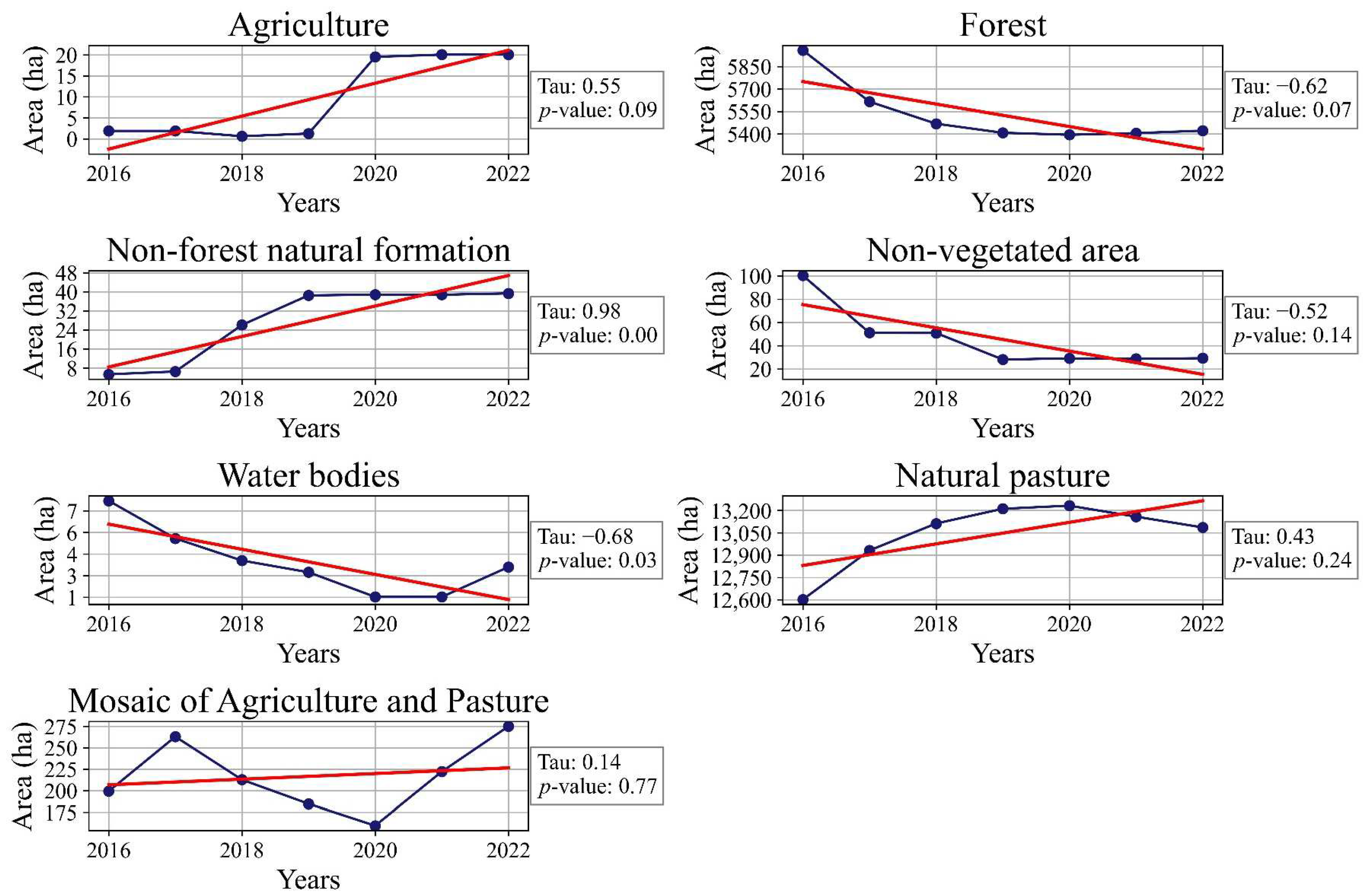
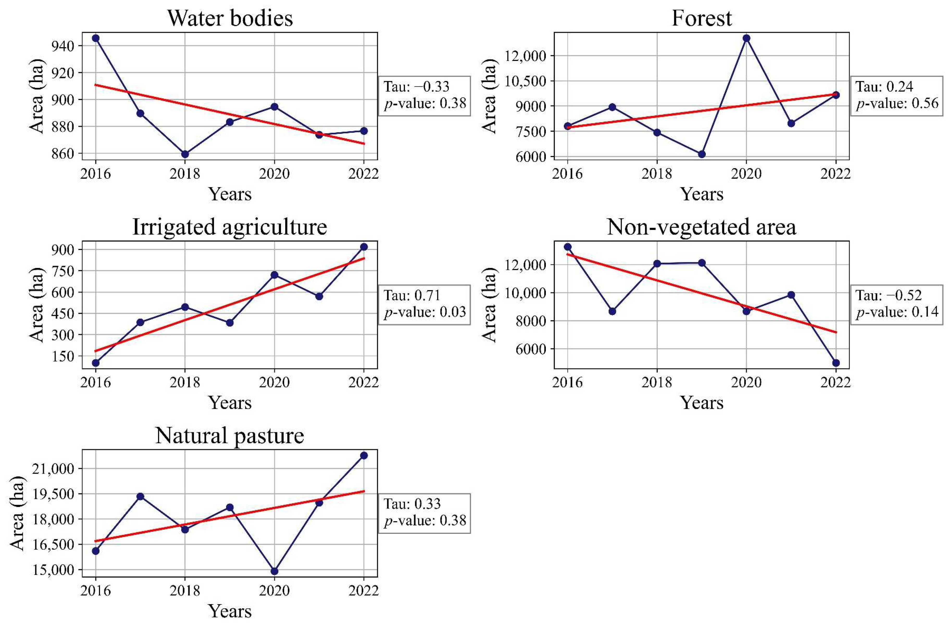
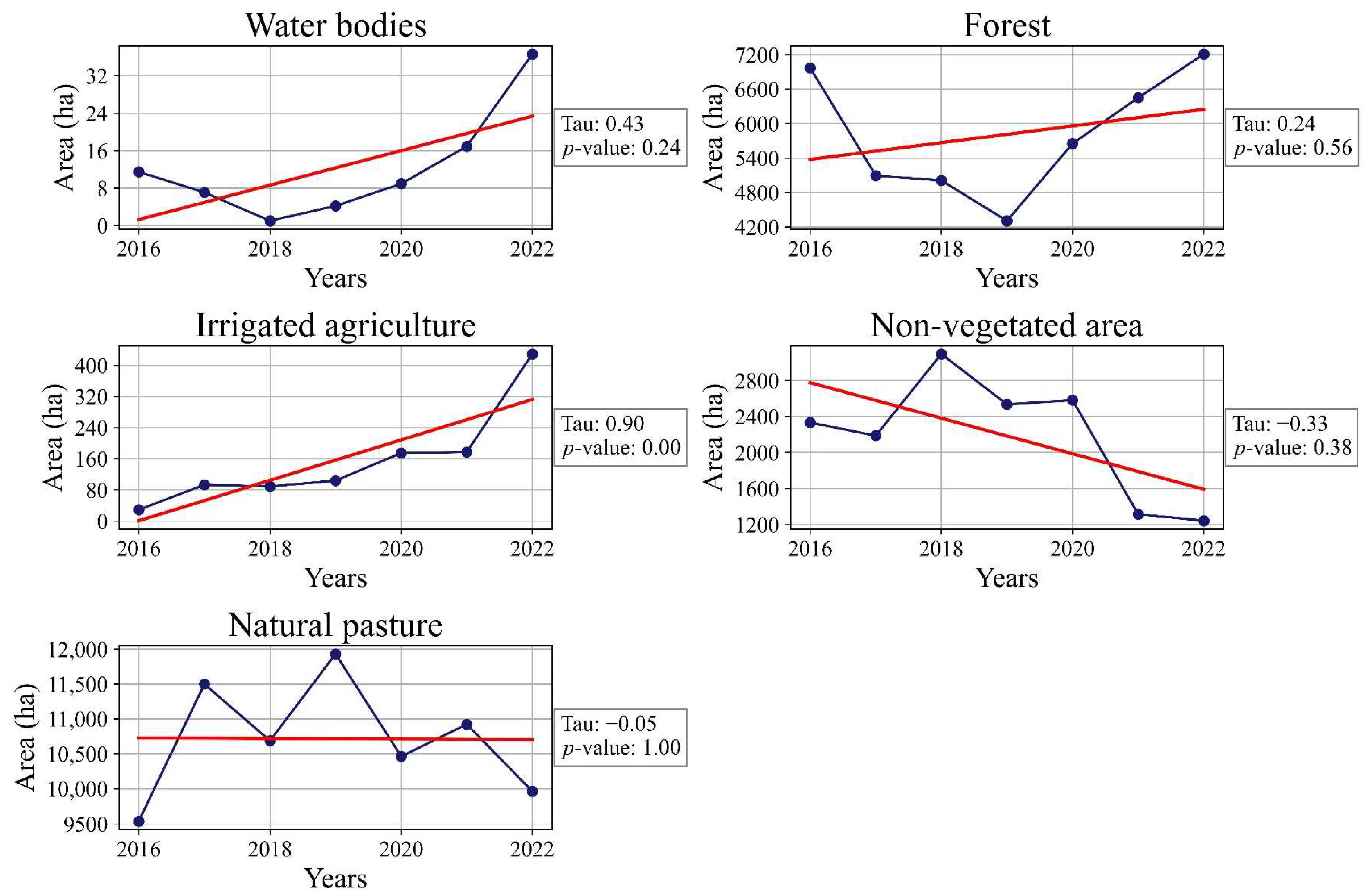
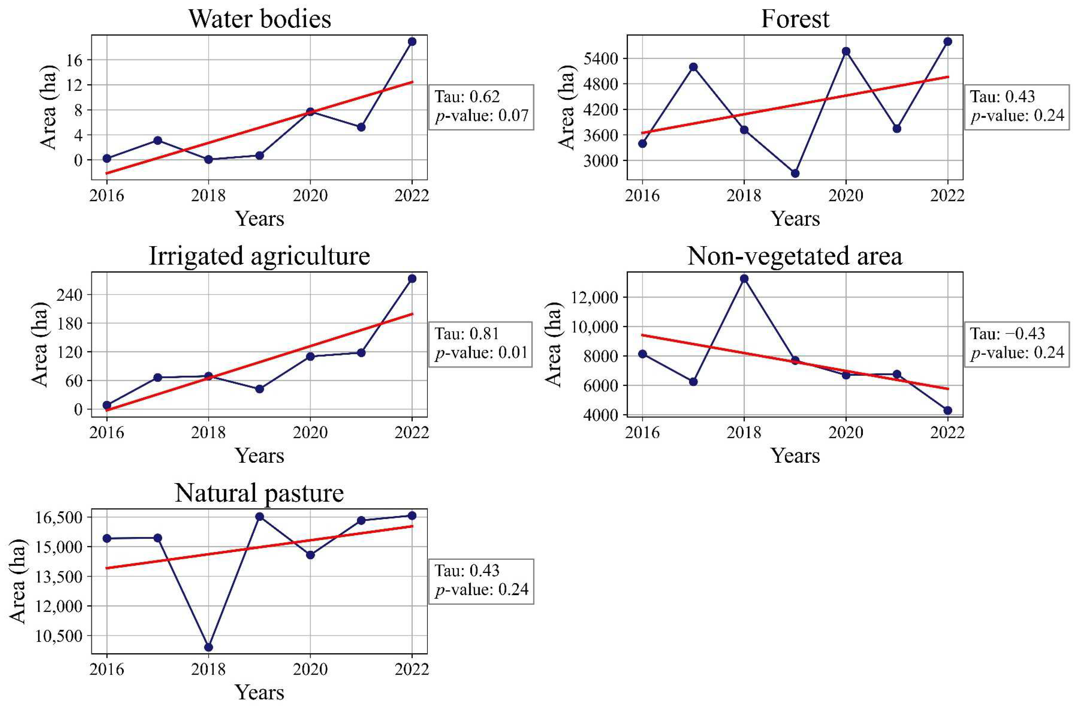
3.6. Temporal and Spatial Analysis of Irrigated Areas (Random Forest)

The LULC maps generated by the Random Forest model exhibit distinct characteristics compared to the MapBiomas maps due to differences in both temporal scale and spatial resolution. MapBiomas operates at an annual scale with a 30 m resolution, while Random Forest uses quarterly Sentinel-2 images from October to December (the dry season in the region), with a 10 m resolution. This is reflected in the predominance of exposed soil and non-vegetated areas represented by the yellow color (Figure 17). The irrigated agricultural areas are small and difficult to visualize, mostly concentrated near the canal’s edges. In the northeast of the maps of Section I, there is a region with a larger area classified as irrigated agriculture, farther from the canal. However, these areas are depressions with accumulated soil moisture, as confirmed through field visits, and represent a limitation of the model due to spectral confusion between the natural vegetation of wetland areas and irrigated zones. The years 2016 and 2018 were the years with the highest amount of exposed soil in Section I of the canal. The forest class showed large annual variations, which is a typical feature of Caatinga vegetation. A significant increase in native forests can be observed in 2020, due to the higher precipitation that occurred that year.
Section II of the canal shows a predominance of the forest and natural pasture classes (Figure 17). As in the previous section, the irrigated agriculture areas are small and are concentrated closer to the canal’s banks. Irrigated agriculture was less than 30 ha in 2016, with noticeable growth in the following years. The year 2022 shows irrigated agriculture areas further away from the canal’s edge. This year is also characterized by higher precipitation, which may have caused greater soil moisture accumulation, consequently leading to spectral confusion, as observed in Section I.
By observing the areas in hectares for each class in Section I of the Canal do Sertão Alagoano, a significant trend of increase in irrigated agriculture between 2016 and 2022 is noted (p < 0.05), with a τ coefficient of 0.71 (Figure 18). In 2016, the areas of irrigated agriculture identified in Section I of the canal by the Random Forest model were 101 ha, reaching their peak in 2022 with 918 ha. Natural pasture and forests showed slight growth in this section of the canal, both of which were not significant (p > 0.05).
Irrigated agriculture has been growing in Section II of the canal, with a significant trend according to the Mann–Kendall statistical analysis, with a τ of 0.90 and a p-value < 0.05 (Figure 19). The Random Forest model identified an approximate area of 29 ha of irrigated agriculture in 2016, with a significant increase in this area until 2022, reaching approximately 429 ha. Pasture in this section of the canal did not show a significant trend of growth or decline according to the Mann–Kendall analysis (p > 0.05).
In Section III of the canal, the dominant class is natural pasture (Figure 20). The areas of irrigated agriculture follow the same pattern as in Sections I and II, with small areas located near the canal’s edges. This section has a larger total irrigated area compared to the second section. However, since the total area is also larger, this justifies the difference. It is noticeable that the southeastern region of the map shows large non-vegetated areas, a problem that was more pronounced in 2018 but has gradually decreased in the following years. These areas may have potential for irrigated agriculture, depending on factors such as topography and soil characteristics, and could become locations where irrigation intensifies in the future. In Section IV of the Sertão Canal (Figure 20), it is possible to see the continuation of the non-vegetated soil areas that begin in the southeast of the maps of Section III. This section of the canal has the smallest area of irrigated agriculture, a feature explained by it being the most recent section of the canal to be completed. Small irrigated areas are observed along the canal’s edge. The denser forest vegetation remains virtually unchanged, indicating that the expansion of irrigated agriculture has not interfered with this native vegetation during the evaluated period. Changes in the forest class are more related to variations in precipitation over the years.
The irrigated agriculture class showed a significant growth trend in Section III of the canal (p < 0.05), with a τ value of 1, demonstrating constant growth, increasing from 38 ha in 2016 to approximately 491 ha in 2022 (Figure 21). The natural pasture class did not show a significant growth or decrease trend according to the Mann–Kendall statistical analysis (p > 0.05).
In Section IV, as in the previous sections, irrigated agriculture has been growing significantly over the years evaluated (p < 0.05), increasing from 8 ha in 2016 to approximately 273 ha in 2022, with a τ coefficient of 0.81 (Figure 22). The natural pasture class showed slight growth, but it was not significant (p > 0.05).

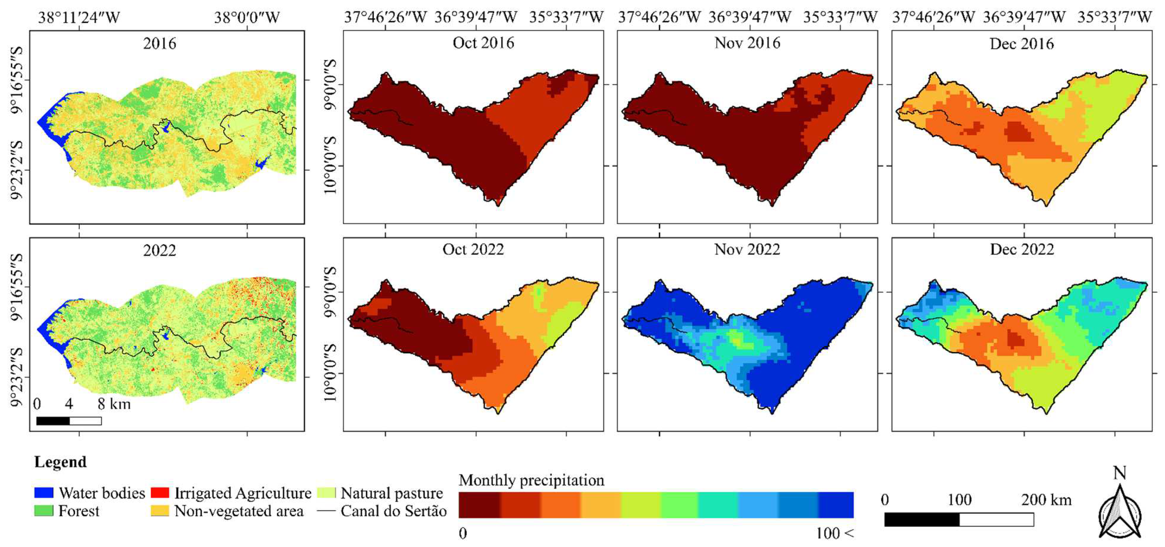
3.7. Seasonal Precipitation Variations: Comparison Between Wet and Dry Periods

When evaluating the maps of annual accumulated precipitation generated using data from the TerraClimate model, it was possible to identify the wettest and driest years during the study period, with the goal of analyzing the influence of precipitation on the LULC results generated by the Random Forest model. The years 2020 and 2022 were the wettest, with accumulated precipitation in areas near the Canal do Sertão Alagoano ranging from 700 to over 1000 mm per year (Figure 23). These data correlate with the LULC maps, which showed an increase in forest areas in these same years, as well as a decrease in non-vegetated areas. In contrast, 2016 and 2018 were dry years, resulting in an increase in exposed soil areas (i.e., non-vegetated areas) across all sections of the Canal do Sertão Alagoano. The analysis of the monthly precipitation maps for October, November, and December indicates that in 2022, the average monthly precipitation was 21.56 mm, 98.49 mm, and 50.77 mm, respectively, values higher than those recorded in 2020, which were 12.66 mm, 40.97 mm, and 27.67 mm. However, 2020 had a larger forest area than 2022. The explanation for this behavior could be the cloud filtering process used, as the months of November and December of 2022 had a high percentage of cloud cover, and the Sentinel-2 image mosaic for this year was generated using images from October, the driest month among the three months of that year. In 2020, rainfall occurred in November, and although it was not very intense, it was sufficient to influence the Caatinga forest vegetation, which responds very quickly to precipitation, with the mosaic for that year being generated using images from all three months evaluated.
Figure 24 shows the contrast of the Caatinga vegetation between the wet and dry periods in a small area of Section I of the Canal do Sertão Alagoano. In the first map, the vegetation appears green and healthier, which is reflected in the LULC map for the same period generated by the Random Forest model. The LULC map shows a larger area of forest and agriculture. The non-vegetated areas (exposed soil) are small and have well-defined geometric shapes, likely representing areas of rainfed agriculture that have already been harvested, leaving the soil exposed, or areas being prepared for planting. In contrast, the map for the dry period shows earthy tones, with little vegetation, which is more open and sparser, resulting in a larger amount of exposed soil. The exposed soil class stands out significantly in the LULC map for the dry period, where areas that previously had agriculture have been harvested, and the soil is now uncovered.
Figure 25 shows the contrast between the years 2016 and 2022, representing a dry year and a rainy year, respectively. The year 2016 was a dry year throughout the north-eastern region of Brazil, and as seen in Figure 25, the three months of the period used to generate the Sentinel-2 mosaic for this study were extremely dry. This is reflected in the vegetation, as observed in the LULC map for this year, where the presence of non-vegetated areas stands out and predominates in much of the map for Section I of the canal. In that year, non-vegetated areas totaled 13,265.13 ha, while forest and natural pasture covered 7805.21 ha and 16,098.16 ha, respectively. Irrigated agriculture was minimal, with only 100.99 ha, and water bodies totaled 945.68 ha. The year 2022 is the opposite, with rainy months during the dry period evaluated, which influenced the increase in forest and pasture areas. Forest reached 9655.11 ha, natural pasture expanded to 21,769.26 ha, and non-vegetated areas decreased to 4996.03 ha. Irrigated agriculture also grew, occupying 918.18 ha, while water bodies slightly reduced to 876.59 ha. This demonstrates how the Caatinga, the exclusive biome of Brazil’s semi-arid region, is versatile and adapts to climatic conditions. The Caatinga forest loses its leaves during the dry period to stay alive, reducing energy expenditure and water loss. On the other hand, even small amounts of rainfall are capable of changing this scenario, with the vegetation turning green again through rapid leaf growth and development of this highly adapted native vegetation.

4. Discussion

4.1. MapBiomas

According to MapBiomas data, the total agriculture area across all sections of the canal increased from 78 ha in 2016 to 368 ha in 2022. These values are very small and do not reflect the actual conditions of the region, as, according to the Brazilian Institute of Geography and Statistics (IBGE), the area allocated to temporary agriculture in 2022 was 11,585 hectares, considering only the municipalities of Água Branca, Delmiro Gouveia, Inhapi, and São José da Tapera (https://sidra.ibge.gov.br/pesquisa/pam/tabelas; accessed on 13 March 2025).
When evaluating the performance of MapBiomas, a high accuracy was observed in identifying forests, natural pastures, non-vegetated areas, and water bodies, with precision above 80% for all these classes. A study conducted by Viana et al. [18] assessed the accuracy of MapBiomas LULC maps, reporting a user accuracy above 80% for the evaluated classes, which corroborates the findings of this study. This result highlights the importance of this tool for environmental monitoring, tracking changes in forest vegetation, and monitoring deforestation.
On the other hand, its performance in classifying agricultural areas in the Alagoan backcountry is still limited, achieving only 41% precision, which leads to an underestimation of these areas. This result is corroborated by the validation performed by MapBiomas itself, which shows that in 2022, for MapBiomas Collection 8, only 21.53% of the area mapped as agriculture in the Caatinga is actually agriculture (https://brasil.mapbiomas.org/estatistica-de-acuracia/colecao-8/; accessed on 13 March 2025). However, for the Cerrado and Atlantic Forest biomes, in 2022, the area classified as agriculture that was actually agriculture was 92.88% and 86.73%, respectively.
The semi-arid region of Brazil exhibits sudden changes in vegetation according to precipitation patterns. This characteristic complicates the identification of agricultural areas in satellite images, especially when working with annual averages, as in the case of MapBiomas. Under these conditions, areas that belong to a given class only for part of the year tend to be underrepresented or even discarded in the annual average, since pixels are classified based on the frequency of observations throughout the year. If the class of interest appears for a short period compared to other predominant classes, its occurrence is diluted or replaced in the final classification. Another factor that may affect the effectiveness of MapBiomas is the seasonality of agriculture in the region, which occurs mainly during the rainy season when the high presence of clouds hinders the visualization of land use and land cover (LULC) in satellite images. These two factors highlight the challenges of using annual averages, as rainfed agriculture, which is concentrated in the short rainy period, ends up being masked due to its reduced representation throughout the year and its overlap with a period of intense cloud cover.
When working with long-cycle crops such as sugarcane, MapBiomas demonstrated high classification performance in the central–southern region of Brazil, with an 84.7% agreement between actual and estimated data [19]. However, in the semi-arid region of Alagoas, field visits revealed that short-cycle crops (e.g., beans, corn, watermelon, and squash, among others) predominate. These crops tend to be suppressed in models that rely on annual averages, such as MapBiomas, when another class appears more frequently throughout the year.
Another factor that affected the identification of agricultural areas in the region is the small size of these areas. According to data provided by SEMARH, 93% of the properties that use water from the canal for irrigation range between 0.1 and 5 ha. The medium resolution of satellite images makes it difficult to visualize these small properties. Velpuri et al. [20] evaluated the precision of irrigated agriculture classification using satellite images with different spatial resolutions and concluded that higher-resolution images performed better in identifying irrigated areas. Gumma et al. [21] highlighted that low-resolution images tend to mix multiple classes within a single pixel, leading to a loss in the identification of smaller and more fragmented irrigated areas. This knowledge is particularly important in semi-arid regions where irrigation is still developing, such as along the Canal do Sertão Alagoano, where irrigated areas are small.
The MapBiomas model was not suitable for identifying irrigated agriculture areas along the Canal do Sertão Alagoano. This is because it operates on an annual scale, with averages generated from observations throughout the entire year. Irrigated agriculture, however, primarily occurs during the dry season in the region, while rainfed agriculture predominates during the rainy season. If MapBiomas provided monthly data, it would be possible to evaluate agriculture exclusively during the dry months, and the agricultural activity identified in this period would correspond to the region’s irrigated agriculture. This methodology is similar to the one used by Magidi et al. [8], who achieved 88% precision in classifying irrigated areas during the dry season in eastern South Africa.
MapBiomas provides irrigated area maps but does not distinguish between irrigated and rainfed agriculture in its main LULC data. However, studies such as the one by Martins et al. [14] demonstrate that with a thorough understanding of the analyzed areas and integration with other data sources, it is possible to classify irrigated agriculture under specific conditions. Another example is the study by Jardim et al. [15], which used MapBiomas LULC data in the municipality of Petrolina. The authors were already aware of the predominance of irrigated perimeters primarily dedicated to fruit growing, and this characteristic was confirmed through evapotranspiration estimated by the SEBAL model and vegetation index analysis. Therefore, although MapBiomas does not directly provide this distinction, its data can serve as a foundation for identifying irrigated areas in integrated methodologies.

4.2. Random Forest

The Random Forest model has the advantage of being adjustable to the specific conditions of the study area, with training samples being manually generated and individually for each year, which improves accuracy when the model is well calibrated. In this study, the Random Forest model was calibrated for the dry season of the region, precisely because it is the period when irrigated agriculture is concentrated [5,8], and there is less cloud cover, which could hinder the acquisition of high-quality satellite images.
The SEMARH data, although collected in a census-like manner where irrigators voluntarily registered, are actual field data that help understand irrigated agriculture in the region and the correlation between the irrigated area from Random Forest and these real data. The model validation with SEMARH data indicated a correlation for the total annual irrigated area (r = 0.85, R2 = 0.73) and for the evaluation of smaller sections (r = 0.81, R2 = 0.65). These lower R2 values may be correlated with several factors, such as the voluntary nature of the SEMARH registration, meaning not all irrigators using the canal’s water are registered. Additionally, the model’s limitations in lowland areas may contribute to this R2 performance.
The NDVI of the land use and land cover (LULC) classes showed values consistent with what was expected for each category. In the native forest, which is the Caatinga, the average NDVI ranged from 0.23 to 0.37, which aligns with the findings of Francisco et al. [22], who in their study showed that NDVI values above 0.37 indicate very dense tree vegetation, while NDVI values between 0.22 and 0.25 correspond to open shrubland–subshrub vegetation. Between 2016 and 2019, the average NDVI values observed in this study were lower than those in 2020 and 2021 (Figure 9). When analyzing the precipitation data, it is noticeable that from October to December of those years, the rainfall indices were lower than in the subsequent years (Figure 23). This reduction in precipitation may have caused the Caatinga to exhibit characteristics similar to the open shrubland–subshrub vegetation described by Francisco et al. [22], resulting in lower NDVI values. These results indicate a good agreement between the LULC data obtained by the Random Forest model and the expected NDVI behavior for each class.
Irrigated agriculture showed quartile values in the boxplot between 0.25 and 0.49, accompanied by high variability, reflecting the diversity in agricultural practices and cultivated crops, as observed in interviews with irrigators and field visits. Magidi et al. [8] used an NDVI threshold between 0.19 and 0.25 to distinguish irrigated areas from non-irrigated ones, which was outside the quartile range observed in this study. In turn, Nhamo et al. [23] adopted an NDVI threshold of 0.14, classifying crops that exceeded this value as irrigated, achieving a precision of 71% in the irrigated area map generated.
Field visits revealed that out of the 33 points classified as irrigated agriculture, 25 were correct and 8 had classification errors. In contrast, MapBiomas showed lower precision in the field visits, failing to identify agriculture in any of the 12 points analyzed. The field results, along with precision metrics and the F1 score, indicate that the Random Forest model outperformed in classifying agriculture. Although Random Forest is one of the methods used in MapBiomas classification, it is important to highlight the differences between the methodologies used. Random Forest was trained to identify agriculture during the dry season, and since it is irrigated, this category stands out more easily compared to other land uses in the semi-arid region. Additionally, the difference in image resolution also influences the classification performance, especially because the region is characterized by small property sizes, as indicated by SEMARH data.
The classification of irrigated agriculture performs better in semi-arid regions, where irrigation has a significant impact on the vegetation’s phenology [24]. The largest classification errors occur in regions with high precipitation and areas with higher soil moisture levels, especially where pasture areas, forests, and irrigated crops mix, presenting similar spectral signatures [9,24,25].
The results of this study highlight the potential of models that are adapted and calibrated for specific regional contexts. However, it was observed that the model struggled in floodplain regions, where the vegetation shows a spectral response similar to that of irrigated agriculture due to higher soil moisture levels. Under these conditions, there may be an overestimation of irrigated areas [9]. This confusion in the model is similar to the errors observed by Biggs et al. [24], where some vegetation types exhibited spectral responses similar to those of irrigated areas due to precipitation and moisture. Knauer et al. [4] also identified an overestimation in the classification of irrigated areas, caused by the model’s confusion in regions near rivers, where the vegetation had a spectral response similar to that of irrigated areas. During field visits to areas benefiting from the Canal do Sertão Alagoano, local farmers reported that in these floodplain areas, the population tends to plant rainfed crops to take advantage of the natural soil moisture and avoid the costs of irrigation.
These findings highlight the importance of incorporating additional environmental variables to improve classification accuracy. Future studies could benefit from a more complex integration of factors such as topography, soil moisture indices, available soil water, and vegetation indices, which may help mitigate the spectral confusion observed in floodplain regions. Deines et al. [11] demonstrated how integrating diverse variables, including soil data, topographic information, spectral indices, and available soil water, can help reduce spectral confusion when identifying irrigated crops. Similarly, Ozdogan et al. [26] emphasized the relevance of temporal information related to crop phenological stages, such as planting, maturation, and harvest, to better distinguish irrigated crops from naturally moist areas. They also suggest that radar imagery, due to its sensitivity to soil moisture even in complex environments, can be a valuable tool in addressing these classification challenges.
Given these limitations, more advanced approaches, such as deep learning techniques, have been increasingly employed in the identification of irrigated agricultural areas, achieving higher precision due to the use of large volumes of data and complex neural networks [27]. Future studies could compare the performance of deep learning techniques with those of machine learning, which were used in this study, and assess the benefits and challenges of each technique, as well as the best outcomes in mapping irrigated areas along the Canal do Sertão Alagoano. We acknowledge that the difference in spatial resolution between MapBiomas data (30 m) and Sentinel-2 imagery (10 m) may affect the comparability of results; therefore, we encourage future research to evaluate the impact of image resolution on the classification of irrigated areas in the Brazilian semi-arid region.

5. Conclusions

MapBiomas exhibited lower precision in identifying agricultural areas in the semi-arid region of Alagoas. Additionally, the fact that this tool operates exclusively at an annual scale limits its ability to detect irrigated agriculture, which predominantly occurs during the dry months of the year. Thus, when dealing with long-cycle crops, large agricultural areas, or environmental studies focused on other land cover classes, the MapBiomas platform proves to be an efficient and accessible alternative for obtaining land use and land cover data. However, for the classification of irrigated areas, MapBiomas products can serve as a baseline within integrated methodologies that incorporate additional complementary data. It is important to highlight that this study utilized MapBiomas Collection 8, and more recent or future versions of the model may enhance calibration and improve performance in classifying agricultural areas in the semi-arid region.
The Random Forest model, calibrated for the study area and specific conditions, demonstrated higher precision than MapBiomas in classifying agricultural areas. It was effectively used to identify irrigated agriculture during the region’s dry period, with validation conducted through field visits. Random Forest stands out as a more efficient tool for classifying irrigated areas, offering the advantage of being adaptable to specific conditions. However, the model exhibited limitations in lowland areas, where high soil moisture levels promote vegetation growth with spectral responses similar to irrigated crops, leading to classification errors.
For future studies, it is recommended that more complex methods be applied to investigate in greater depth the interactions between climatic, hydrological, topographic, and land use factors that influence agricultural dynamics in semi-arid environments.

Author Contributions

Conceptualization, J.L.P.d.S., G.d.N.A.J. and A.C.d.S.A.; methodology, J.L.P.d.S., G.d.N.A.J., F.B.d.S.J., J.B.A.d.S., A.C.d.S.A., T.G.F.d.S., P.R.G., M.V.d.S. and R.M.; software, J.L.P.d.S., F.B.d.S.J., J.B.A.d.S., M.V.d.S. and C.H.S.; validation, J.L.P.d.S., F.B.d.S.J., J.B.A.d.S., G.d.N.A.J. and C.H.S.; formal analysis, J.L.P.d.S., G.d.N.A.J. and A.C.d.S.A.; investigation, J.L.P.d.S., G.d.N.A.J., J.B.A.d.S., C.H.S. and A.C.d.S.A.; resources, G.d.N.A.J. and A.C.d.S.A.; data curation, J.L.P.d.S., J.B.A.d.S., F.B.d.S.J., C.H.S., G.d.N.A.J. and A.C.d.S.A.; writing—original draft preparation, J.L.P.d.S., G.d.N.A.J., T.G.F.d.S., R.M., P.R.G. and A.C.d.S.A.; writing—review and editing, J.L.P.d.S., G.d.N.A.J., T.G.F.d.S., M.V.d.S., R.M., P.R.G. and A.C.d.S.A.; visualization, J.L.P.d.S., G.d.N.A.J., F.B.d.S.J., C.H.S., T.G.F.d.S., M.V.d.S., R.M., P.R.G. and A.C.d.S.A.; supervision, G.d.N.A.J., T.G.F.d.S., M.V.d.S., R.M., P.R.G. and A.C.d.S.A.; project administration, A.C.d.S.A.; funding acquisition, A.C.d.S.A. All authors have read and agreed to the published version of the manuscript.

Funding

This research received funding of the: Coordination for the Improvement of Higher Education Personnel—CAPES (Grant/Award Number: Finance Code 001), Alagoas State Research Support Foundation—FAPEAL (Grant/Award Numbers: N.04/2021-E:60030.0000000218/2022; N.02/2022-E:60030.0000002548/2022; N.11/2022-60030.0000000321/2023; N.38/2022—E:60030.0000002027/2023), and National Council for Scientific and Technological Development—CNPq, (Grant/Award Numbers: N.1728/2022-88881.708029/2022-01; N.2398/2022-88881.691704/2022-01; N.11/2022-60030.0000000321/2023).

Data Availability Statement

The original contributions presented in the study are included in the article; further inquiries can be directed to the corresponding author.

Acknowledgments

We acknowledge the Programa de Pós-Graduação em Agronomia (PPGA) and the Laboratório de Irrigação e Agrometeorologia (LIA) of the Universidade Federal de Alagoas (UFAL) for supporting the development of this research.

Conflicts of Interest

The authors declare no conflicts of interest.

References

  1. De Souza Medeiros, A.; Gonzaga, G.B.M.; da Silva, T.S.; de Souza Barreto, B.; dos Santos, T.C.; de Melo, P.L.A.; de Araújo Gomes, T.C.; Maia, S.M.F. Changes in Soil Organic Carbon and Soil Aggregation Due to Deforestation for Smallholder Management in the Brazilian Semi-Arid Region. Geoderma Reg. 2023, 33, e00647. [Google Scholar] [CrossRef]
  2. Carvalho, A.L.; Araújo-Neto, R.A.; Lyra, G.B.; Cerri, C.E.P.; Maia, S.M.F. Impact of Rainfed and Irrigated Agriculture Systems on Soil Carbon Stock under Different Climate Scenarios in the Semi-Arid Region of Brazil. J. Arid. Land 2022, 14, 359–373. [Google Scholar] [CrossRef]
  3. Halder, S.; Das, S.; Basu, S. Use of Support Vector Machine and Cellular Automata Methods to Evaluate Impact of Irrigation Project on LULC. Environ. Monit. Assess. 2023, 195, 3. [Google Scholar] [CrossRef]
  4. Knauer, K.; Gessner, U.; Fensholt, R.; Forkuor, G.; Kuenzer, C. Monitoring Agricultural Expansion in Burkina Faso over 14 Years with 30 m Resolution Time Series: The Role of Population Growth and Implications for the Environment. Remote Sens. 2017, 9, 132. [Google Scholar] [CrossRef]
  5. Traoré, F.; Bonkoungou, J.; Compaoré, J.; Kouadio, L.; Wellens, J.; Hallot, E.; Tychon, B. Using Multi-Temporal Landsat Images and Support Vector Machine to Assess the Changes in Agricultural Irrigated Areas in the Mogtedo Region, Burkina Faso. Remote Sens. 2019, 11, 1442. [Google Scholar] [CrossRef]
  6. Dangui, K.; Jia, S. Water Infrastructure Performance in Sub-Saharan Africa: An Investigation of the Drivers and Impact on Economic Growth. Water 2022, 14, 3522. [Google Scholar] [CrossRef]
  7. Zhao, Y.; An, R.; Xiong, N.; Ou, D.; Jiang, C. Spatio-Temporal Land-Use/Land-Cover Change Dynamics in Coastal Plains in Hangzhou Bay Area, China from 2009 to 2020 Using Google Earth Engine. Land 2021, 10, 1149. [Google Scholar] [CrossRef]
  8. Magidi, J.; Nhamo, L.; Mpandeli, S.; Mabhaudhi, T. Application of the Random Forest Classifier to Map Irrigated Areas Using Google Earth Engine. Remote Sens. 2021, 13, 876. [Google Scholar] [CrossRef]
  9. Ragettli, S.; Herberz, T.; Siegfried, T. An Unsupervised Classification Algorithm for Multi-Temporal Irrigated Area Mapping in Central Asia. Remote Sens. 2018, 10, 1823. [Google Scholar] [CrossRef]
  10. Gumma, M.K.; Thenkabail, P.S.; Teluguntla, P.G.; Oliphant, A.; Xiong, J.; Giri, C.; Pyla, V.; Dixit, S.; Whitbread, A.M. Agricultural Cropland Extent and Areas of South Asia Derived Using Landsat Satellite 30-m Time-Series Big-Data Using Random Forest Machine Learning Algorithms on the Google Earth Engine Cloud. GIsci. Remote Sens. 2020, 57, 302–322. [Google Scholar] [CrossRef]
  11. Deines, J.M.; Kendall, A.D.; Crowley, M.A.; Rapp, J.; Cardille, J.A.; Hyndman, D.W. Mapping Three Decades of Annual Irrigation across the US High Plains Aquifer Using Landsat and Google Earth Engine. Remote Sens. Environ. 2019, 233, 111400. [Google Scholar] [CrossRef]
  12. Phalke, A.R.; Özdoğan, M.; Thenkabail, P.S.; Erickson, T.; Gorelick, N.; Yadav, K.; Congalton, R.G. Mapping Croplands of Europe, Middle East, Russia, and Central Asia Using Landsat, Random Forest, and Google Earth Engine. ISPRS J. Photogramm. Remote Sens. 2020, 167, 104–122. [Google Scholar] [CrossRef]
  13. Neves, A.K.; Körting, T.S.; Fonseca, L.M.G.; Escada, M.I.S. Assessment of TerraClass and MapBiomas Data on Legend and Map Agreement for the Brazilian Amazon Biome. Acta Amaz. 2020, 50, 170–182. [Google Scholar] [CrossRef]
  14. Martins, M.A.; Tomasella, J.; Bassanelli, H.R.; Paiva, A.C.E.; Vieira, R.M.S.P.; Canamary, E.A.; Alvarenga, L.A. On the Sustainability of Paddy Rice Cultivation in the Paraíba Do Sul River Basin (Brazil) under a Changing Climate. J. Clean. Prod. 2023, 386, 135760. [Google Scholar] [CrossRef]
  15. Jardim, A.M.d.R.F.; Araújo Júnior, G.d.N.; Silva, M.V.d.; Santos, A.d.; Silva, J.L.B.d.; Pandorfi, H.; Oliveira-Júnior, J.F.d.; Teixeira, A.H.d.C.; Teodoro, P.E.; de Lima, J.L.M.P.; et al. Using Remote Sensing to Quantify the Joint Effects of Climate and Land Use/Land Cover Changes on the Caatinga Biome of Northeast Brazilian. Remote Sens. 2022, 14, 1911. [Google Scholar] [CrossRef]
  16. Kavzoglu, T.; Bilucan, F. Effects of Auxiliary and Ancillary Data on LULC Classification in a Heterogeneous Environment Using Optimized Random Forest Algorithm. Earth Sci. Inf. 2023, 16, 415–435. [Google Scholar] [CrossRef]
  17. Montesinos-López, O.A.; Kismiantini; Alemu, A.; Montesinos-López, A.; Montesinos-López, J.C.; Crossa, J. Balancing Sensitivity and Specificity Enhances Top and Bottom Ranking in Genomic Prediction of Cultivars. Plants 2025, 14, 308. [Google Scholar] [CrossRef] [PubMed]
  18. Viana, J.F.d.S.; Montenegro, S.M.G.L.; Srinivasan, R.; Santos, C.A.G.; Mishra, M.; Kalumba, A.M.; da Silva, R.M. Land Use and Land Cover Trends and Their Impact on Streamflow and Sediment Yield in a Humid Basin of Brazil’s Atlantic Forest Biome. Diversity 2023, 15, 1220. [Google Scholar] [CrossRef]
  19. Guarenghi, M.M.; Garofalo, D.F.T.; Seabra, J.E.A.; Moreira, M.M.R.; Novaes, R.M.L.; Ramos, N.P.; Nogueira, S.F.; de Andrade, C.A. Land Use Change Net Removals Associated with Sugarcane in Brazil. Land 2023, 12, 584. [Google Scholar] [CrossRef]
  20. Velpuri, N.M.; Thenkabail, P.S.; Gumma, M.K.; Biradar, C.; Dheeravath, V.; Noojipady, P.; Yuanjie, L. Influence of Resolution in Irrigated Area Mapping and Area Estimation. Photogramm. Eng. Remote Sens. 2009, 75, 1383–1395. [Google Scholar] [CrossRef]
  21. Gumma, M.K.; Thenkabail, P.S.; Hideto, F.; Nelson, A.; Dheeravath, V.; Busia, D.; Rala, A. Mapping Irrigated Areas of Ghana Using Fusion of 30 m and 250 m Resolution Remote-Sensing Data. Remote Sens. 2011, 3, 816–835. [Google Scholar] [CrossRef]
  22. Francisco, P.R.M.; Chaves, I.D.B.; Chaves, L.H.G.; de Lima, E.R.V.; da Silva, B.B. Análise Espectral e Avaliação de Índices de Vegetação Para o Mapeamento Da Caatinga. Rev. Verde Agroecol. Desenvolv. Sustentável 2015, 10, 26. [Google Scholar] [CrossRef]
  23. Nhamo, L.; Ebrahim, G.Y.; Mabhaudhi, T.; Mpandeli, S.; Magombeyi, M.; Chitakira, M.; Magidi, J.; Sibanda, M. An Assessment of Groundwater Use in Irrigated Agriculture Using Multi-Spectral Remote Sensing. Phys. Chem. Earth Parts A/B/C 2020, 115, 102810. [Google Scholar] [CrossRef]
  24. Biggs, T.W.; Thenkabail, P.S.; Gumma, M.K.; Scott, C.A.; Parthasaradhi, G.R.; Turral, H.N. Irrigated Area Mapping in Heterogeneous Landscapes with MODIS Time Series, Ground Truth and Census Data, Krishna Basin, India. Int. J. Remote Sens. 2006, 27, 4245–4266. [Google Scholar] [CrossRef]
  25. Maselli, F.; Chiesi, M.; Angeli, L.; Fibbi, L.; Rapi, B.; Romani, M.; Sabatini, F.; Battista, P. An Improved NDVI-Based Method to Predict Actual Evapotranspiration of Irrigated Grasses and Crops. Agric. Water Manag. 2020, 233, 106077. [Google Scholar] [CrossRef]
  26. Ozdogan, M.; Yang, Y.; Allez, G.; Cervantes, C. Remote Sensing of Irrigated Agriculture: Opportunities and Challenges. Remote Sens. 2010, 2, 2274–2304. [Google Scholar] [CrossRef]
  27. Benbahria, Z.; Sebari, İ.; Hajji, H.; Smiej, M.F. Intelligent Mapping of Irrigated Areas from Landsat 8 Images Using Transfer Learning. Int. J. Eng. Geosci. 2021, 6, 40–50. [Google Scholar] [CrossRef]
Figure 1. Location map of Sections I–IV of the Canal do Sertão Alagoano that make up the study area in the interior of the state of Alagoas, Northeast Brazil. Blue line—constructed sections of the canal. The light blue vertical lines indicate the start and end points of each of the four sections analyzed (T1 to T4). Red outlines—study areas corresponding to 10 km-wide buffers (5 km on each side) along the canal’s path within each section.
Agriengineering 07 00134 g001
Figure 2. Methodological flowchart of the study, detailing the stages of data collection, processing, and validation of land use and land cover (LULC) data.
Agriengineering 07 00134 g002
Figure 3. Field validation of irrigated agriculture areas according to the Random Forest model and comparison with LULC from MapBiomas for the same area in 2021. (A) LULC Random Forest 2021. (B) Irrigated pasture area identified in field visits. (C) Irrigated watermelon area identified in field visits. (D) Irrigated corn area identified in field visits. (E) Irrigated bean area identified in field visits. (F) LULC MapBiomas 2021.
Agriengineering 07 00134 g003
Figure 4. Classification of errors and correct predictions of the Random Forest and MapBiomas models based on field visits to irrigated and rainfed agriculture points.
Agriengineering 07 00134 g004
Figure 5. Field validation of irrigated agriculture areas according to the Random Forest model. (A) LULC Random Forest 2021. (B) Rainfed pasture area identified in field visits. (C) Floodplain area identified in field visits. The black dashed square highlights the main area of interest within the floodplain region, where soil moisture accumulates and vegetation remains green during the dry season. (D) Rainfed pasture area identified in field visits.
Agriengineering 07 00134 g005
Figure 6. Correlation between observed irrigated agriculture values (ha) provided by SEMARH and estimated values by the Random Forest model in areas benefiting from the Canal do Sertão Alagoano. Black dots represent annual total irrigated area values for each year in the time series, comparing SEMARH census data with Random Forest estimates.
Agriengineering 07 00134 g006
Figure 7. Segmentation and correlation analysis of irrigated areas along the Canal do Sertão Alagoano, with comparison between SEMARH census data and Random Forest model estimates. (A) Map showing the Canal do Sertão with a 2 km buffer on each side, divided into 1 km segments (from 46 to 59) used for analysis. The LULC classification for 2021 is also displayed. (B) Scatter plot showing the correlation between irrigated area estimates obtained from the Random Forest model and SEMARH census data for each segment shown in panel A.
Agriengineering 07 00134 g007
Figure 8. Normalized Difference Vegetation Index (NDVI) for the four sections of the canal from 2016 to 2022.
Agriengineering 07 00134 g008
Figure 9. Boxplots of NDVI variations during part of the dry season (October to December) for different land use and land cover classes (water, forest, irrigated agriculture, non-vegetated area, and pasture) from the Random Forest model, with one map per year between 2016 and 2022, in the areas served by the Canal do Sertão Alagoano.
Agriengineering 07 00134 g009
Figure 10. Land use and land cover (LULC) map for Sections I and II of the Canal do Sertão Alagoano: Surrounding area within a 5 km radius on each side of the canal’s banks.
Agriengineering 07 00134 g010
Figure 11. Temporal trends and Mann–Kendall analysis for MapBiomas land use and land cover classes in hectares in Section I of the Canal do Sertão Alagoano (2016–2022). The blue line represents the estimated data, and the red line represents the trend line for each class.
Agriengineering 07 00134 g011
Figure 12. Temporal trends and Mann–Kendall analysis for MapBiomas land use and land cover classes in hectares in Section II of the Canal do Sertão Alagoano (2016–2022). The blue line represents the estimated data, and the red line represents the trend line for each class.
Agriengineering 07 00134 g012
Figure 13. Land use and land cover (LULC) map for Sections III and IV of the Canal do Sertão Alagoano: Surrounding area within a 5 km radius on each side of the canal’s banks.
Agriengineering 07 00134 g013
Figure 14. Temporal trends and Mann–Kendall analysis for MapBiomas land use and land cover classes in hectares in Section III of the Canal do Sertão Alagoano (2016–2022). The blue line represents the estimated data, and the red line represents the trend line for each class.
Agriengineering 07 00134 g014
Figure 15. Temporal trends and Mann–Kendall analysis for MapBiomas land use and land cover classes in hectares in Section IV of the Canal do Sertão Alagoano (2016–2022). The blue line represents the estimated data, and the red line represents the trend line for each class.
Agriengineering 07 00134 g015
Figure 16. Comparison between the MapBiomas and Random Forest LULC maps for the years 2016 and 2021 in Section I of the Canal do Sertão Alagoano.
Agriengineering 07 00134 g016
Figure 17. Land use and land cover (LULC) map generated by the Random Forest model for Sections I and II of the Canal do Sertão Alagoano: Surrounding area within a 5 km radius from the canal’s banks.
Agriengineering 07 00134 g017
Figure 18. Temporal trends and Mann–Kendall analysis for land use and land cover classes in hectares generated by the Random Forest model in Section I of the Canal do Sertão Alagoano (2016–2022). The blue line represents the estimated data, and the red line represents the trend line for each class.
Agriengineering 07 00134 g018
Figure 19. Temporal trends and Mann–Kendall Analysis for land use and land cover classes in hectares generated by the Random Forest model in Section II of the Canal do Sertão Alagoano (2016–2022). The blue line represents the estimated data, and the red line represents the trend line for each class.
Agriengineering 07 00134 g019
Figure 20. Land use and land cover (LULC) map generated by the Random Forest model for Sections III and IV of the Canal do Sertão Alagoano: Surrounding area within a 5 km radius from the canal’s banks.
Agriengineering 07 00134 g020
Figure 21. Temporal trends and Mann–Kendall analysis for land use and land cover classes in hectares generated by the Random Forest model in Section III of the Canal do Sertão Alagoano (2016–2022). The blue line represents the estimated data, and the red line represents the trend line for each class.
Agriengineering 07 00134 g021
Figure 22. Temporal trends and Mann–Kendall analysis for land use and land cover classes in hectares generated by the Random Forest model in Section IV of the Canal do Sertão Alagoano (2016–2022). The blue line represents the estimated data, and the red line represents the trend line for each class.
Agriengineering 07 00134 g022
Figure 23. Annual and monthly (October to December) accumulated precipitation maps from the TerraClimate model for Alagoas (2016–2022).
Agriengineering 07 00134 g023
Figure 24. Contrasting LULC maps comparing the wet and dry periods in an area of the municipality of Delmiro Gouveia near the Canal do Sertão Alagoano in the year 2021.
Agriengineering 07 00134 g024
Figure 25. LULC maps of Section I of the Canal do Sertão and monthly precipitation during the dry period for two contrasting precipitation years (2016 and 2022).
Agriengineering 07 00134 g025
Table 1. Number of training polygons used for each LULC class in the Random Forest model, organized by year (2016 to 2022).
ClassYear
2016201720182019202020212022
Water bodies1199991112
Forest82794843341877
Irrigated agriculture255870777236113
Non-vegetated area1513161071345
Natural pasture36352446431342
Table 2. Evaluation results of the MapBiomas model for different land use classes, based on precision, recall, and F1 score metrics. The Kappa metric is provided as a measure of the model’s overall agreement.
KappaClassPrecisionRecallF1 Score
0.74Agriculture0.410.890.56
Non-vegetated area1.000.880.94
Water bodies1.001.001.00
Forest1.000.530.69
Natural pasture0.900.960.93
Table 3. Evaluation results of the Random Forest model for different land use classes, based on precision, recall, and F1 score metrics. The Kappa metric is provided as a measure of the model’s overall agreement.
KappaClassPrecisionRecallF1 Score
0.82Irrigated agriculture0.651.000.79
Non-vegetated area0.850.930.89
Water bodies1.000.920.96
Forest1.000.730.84
Natural pasture0.920.840.88
Disclaimer/Publisher’s Note: The statements, opinions and data contained in all publications are solely those of the individual author(s) and contributor(s) and not of MDPI and/or the editor(s). MDPI and/or the editor(s) disclaim responsibility for any injury to people or property resulting from any ideas, methods, instructions or products referred to in the content.

