In-Field Forage Biomass and Quality Prediction Using Image and VIS-NIR Proximal Sensing with Machine Learning and Covariance-Based Strategies for Livestock Management in Silvopastoral Systems

Abstract

Controlling forage quality and grazing are crucial for sustainable livestock production, health, productivity, and animal performance. However, the limited availability of reliable handheld sensors for timely pasture quality prediction hinders farmers’ ability to make informed decisions. This study investigates the in-field dynamics of Mombasa grass (Megathyrsus maximus) forage biomass production and quality using optical techniques such as visible imaging and near-infrared (VIS-NIR) hyperspectral proximal sensing combined with machine learning models enhanced by covariance-based error reduction strategies. Data collection was conducted using a cellphone camera and a handheld VIS-NIR spectrometer. Feature extraction to build the dataset involved image segmentation, performed using the Mahalanobis distance algorithm, as well as spectral processing to calculate multiple vegetation indices. Machine learning models, including linear regression, LASSO, Ridge, ElasticNet, k-nearest neighbors, and decision tree algorithms, were employed for predictive analysis, achieving high accuracy with R² values ranging from 0.938 to 0.998 in predicting biomass and quality traits. A strategy to achieve high performance was implemented by using four spectral captures and computing the reflectance covariance at NIR wavelengths, accounting for the three-dimensional characteristics of the forage. These findings are expected to advance the development of AI-based tools and handheld sensors particularly suited for silvopastoral systems.

1. Introduction

Efficient pasture and forage management are critical for increasing productivity and profitability in livestock systems. The decision-making regarding pasture management, such as optimal grazing times, requires reliable and up-to-date information based on field conditions, forage yield per unit area, and the nutritional quality of the pasture [1,2].

In-field estimation methods, which involve both direct and indirect measurements of pasture biomass, often lack precision and are unsuitable for grasslands with multistratum arrangements, such as silvopastoral systems, or pastures with species mixtures that exhibit different growth physiologies [3]. For example, tropical pastures in the Caribbean region of Colombia have distinctive stem elongation characteristics, influencing growth and nutritional quality and potentially interfering with results if improper measurement techniques are used.

The most used direct method for biomass estimation is botanical yield estimation (botanical sampling), which involves cutting and weighing pasture forage. While accurate, this method is labor-intensive, time-consuming, and requires numerous samples to ensure reliable results [4]. Indirect methods often rely on visual estimates and tools that correlate plant height and density with biomass production (e.g., disc meters and rulers). However, these methods can yield inaccurate results in tropical forages, mostly related to observer experience and the need for specific calibration equations according to climatic conditions and forage species [3].

The nutritional quality of forages is determined by their chemical composition and digestibility, which can estimate potential intake by animals. Quantifying the nutritional value of forages is typically carried out using various laboratory analytical techniques. These methods require time, skilled personnel, and two key steps: in-field sampling and sample processing laboratory [5]. Official procedures for nutrient quantification require specialized equipment, reagents, time, and supplies. As a result, establishing a nutritional profile for feed may involve several of these methods [6]. The specificity of these analyses means that laboratories may have response times that are not aligned with the quick decision making required by farmers. Near Infrared Reflectance (NIR) technology is a laboratory technique that reduces analysis response times; however, it requires calibration through a robust number of samples, and without these calibrated equations, the results may be unreliable [5].

Traditional methods of estimating pasture biomass and nutritional quality, while reliable, have disadvantages that hinder quick decision making in pasture management. The ability to assess biomass and forage quality is vital for optimizing feeding strategies and ensuring sustainable livestock production. Despite this importance, accessible and reliable tools for in-field prediction remain limited, highlighting the potential use of new technologies to address these challenges.

Recent advancements in optical hyperspectral sensing technologies, including visible imaging and near-infrared (VIS-NIR) spectroscopy, provide new opportunities for rapid, non-destructive, in situ analysis of plant characteristics [6,7]. These technologies, particularly indirect measurements based on VIS-NIR, have the potential to address limitations in forage quality evaluation, such as pasture variability and sample representativeness.

The novelty of this proposed technology lies in its ability to be adjusted in-field to a higher resolution and a smaller scale by positioning it as close as possible to the target area. In contrast, satellite and drone technologies operate at lower resolutions and larger scales and are unable to measure conditions beneath trees, so more research is needed for handheld sensors, as outlined in [8]. Our approach enables a better understanding of the heterogeneity of growth conditions within the silvopastoral system, made possible by the higher resolution of our method, something not achievable with remote sensing technologies. Knowledge of pasture heterogeneity contributes to livestock management by enhancing decision making through more precise and localized data on forage availability and quality, ultimately improving grazing strategies and animal nutrition. This approach minimizes the use of laboratory residuals and enhances the time cost benefit for decision making. When combined with machine learning (ML) models, these technologies form the foundation for artificial intelligence (AI) systems aimed at efficient forage management. The variability of biomass and forage quality in silvopastoral systems limits the applicability of analytical or expert-based models, making machine learning the most suitable alternative due to its ability to process complex data and account for the high variability inherent in these environments [9].

By integrating machine learning with sensor data, farm management systems are transforming into real-time, AI-driven programs that deliver valuable recommendations and insights to support farmers in decision making and action to improve livestock management [10]. By incorporating this technology into specialized software models (such as mobile apps and web platforms), farm management systems can evolve into AI-powered assistants for producers. These intelligent systems process real-time sensor data using machine learning algorithms, providing precise recommendations on forage availability, grazing strategies, and pasture management. This automation reduces the need for manual field assessments, minimizing human labor while enhancing decision-making efficiency and productivity in livestock farming. These advancements are expected to support tools for the Fourth Industrial Revolution, including developments in the Internet of Things (IoT), AI, and ML systems, which farmers could directly operate to improve efficiency and sustainability [10,11,12]. This approach offers a promising solution to overcome the drawbacks of traditional methods, which can be either imprecise or time-consuming.

The advantages of these technologies are particularly evident in silvopastoral systems with scattered trees, where remote sensing technology struggles to capture conditions of the pastures beneath the trees [13]. This highlights the need for further exploration of ground-based technologies for in situ measurements. Handheld and portable equipment, such as handheld spectrometers and smartphone cameras, have the potential to transform how pasture biomass and quality are evaluated in situ by proximal sensing, offering a more precise and objective approach compared to traditional methods and remote sensing technologies. By reducing human error, this approach would enhance the accuracy and consistency of the estimations. These new tools promise to revolutionize pasture management by offering efficient, accurate, and cost-effective solutions to the challenges that have traditionally hindered rapid decision-making in the field.

The aim of this study was to evaluate the use of handled VIS-NIR optical spectrometer, RGB cameras, and machine learning models for the in-field prediction of biomass and forage quality of the Megathyrsus maximus cv. Mombasa, as well as to understand how forage production is influenced by the characteristics of radiation beneath scattered trees. The research explores innovative data collection and processing methods, including image segmentation based on Mahalanobis distance, spectral feature extraction, and data transformation. To enhance model accuracy, a covariance-based error reduction strategy was applied to account for the three-dimensional structure and variability of forage tussock [14]. The main contribution is providing a practical and cost-effective solution for in-field forage biomass and quality prediction in silvopastoral systems, leveraging handheld proximal sensors to overcome the limitations of traditional remote sensing, enabling rapid decision making and supporting sustainable livestock management.

2. Plant Physiology, Spectral Data, and Imaging for Megathyrsus maximus cv. Mombasa Characterization

The relationship between plant physiology and spectral and image data is fundamental for understanding vegetation health, biomass, and the estimation of quality traits [15]. Plant physiology influences how plants absorb, transmit, and reflect light across different wavelengths, which is captured through spectral data obtained from sensors measuring reflectance at specific bands (e.g., visible, near-infrared) [16,17]. These spectral signatures provide insights into chlorophyll content, water status, and stress conditions [18]. Image data derived from visible (RGB), multispectral, or hyperspectral imaging translate this spectral information into spatial patterns, allowing for large-scale assessment of plant traits, growth dynamics, and environmental interactions [7,19]. Integrating these datasets enhances precision in biomass modeling and quality trait estimation.

Remote and proximal sensing techniques, including visible, hyperspectral, and multispectral imagery, UAV (Unmanned Aerial Vehicle)-based systems, and sensor fusion, can effectively estimate grass traits such as biomass, nitrogen fixation, and quality, although the accuracy and applicability of these methods can vary depending on the specific technique and environmental conditions [20].

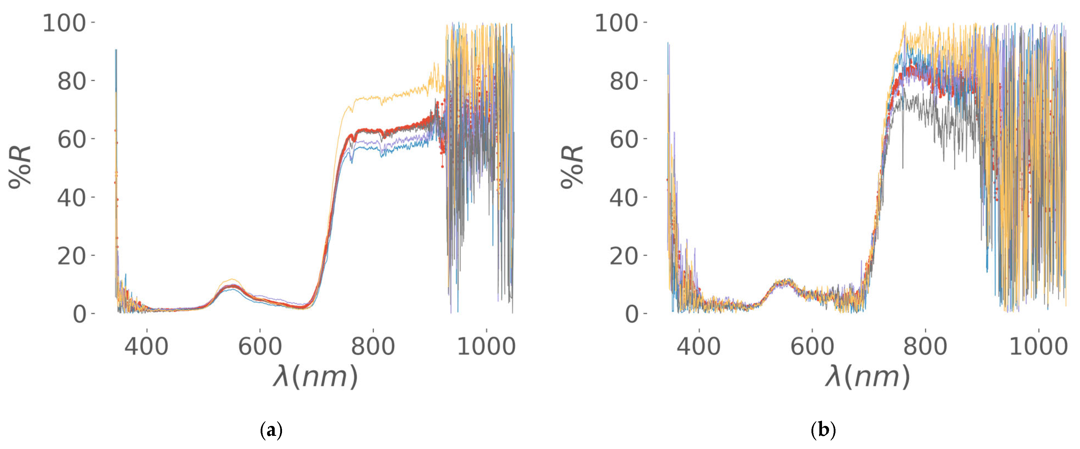
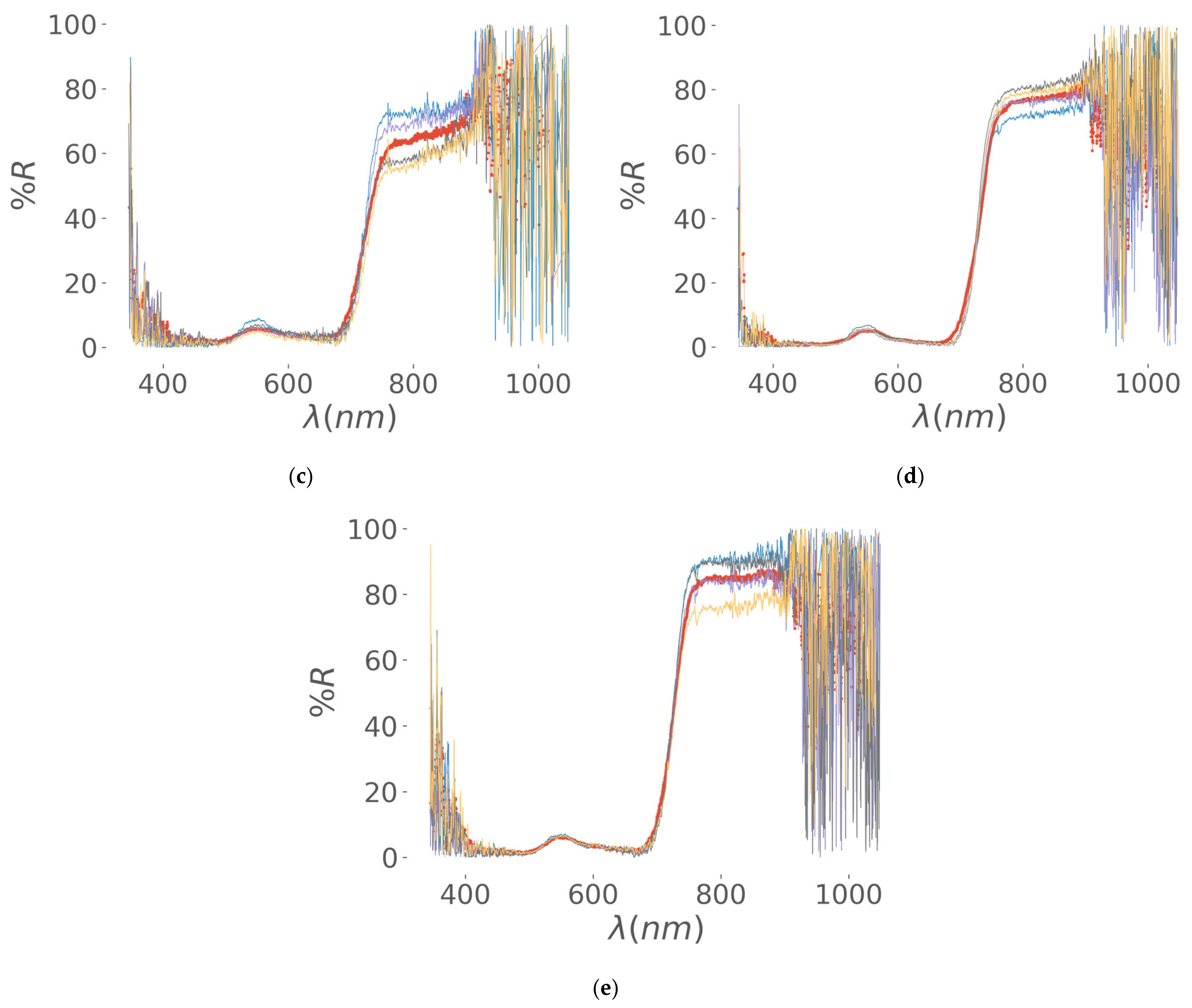
2.1. Plant Spectra for Biomass Estimation and Quality Assessment

Plant spectra can be used to estimate specific traits or as a comprehensive measure of plant form and function [21], with the potential for complementary use when specific traits are known, and reliable models exist for estimation [22]. For instance, blue grama grass canopy can be spectrally estimated for total wet or dry biomass and leaf water content, with best results in the 0.35 to 0.44 m region [23]. Similarly, quality traits of a type of grass such as alfalfa are characterized by several vegetation indexes (VIs) with strong relation with VIS-NIR bands [8]. VI is a mathematical combination of reflectance values at specific wavelengths of spectra used to assess plant health, biomass, and canopy structure from remote or proximal sensing data.

Plant spectra also integrate multiple aspects of their form and function [21]. The information contained in the spectrum can be distilled into estimates of specific traits or used directly. These two approaches can be complementary: the former is most useful when the traits of interest are known in advance and reliable models exist to estimate them, while the latter is more beneficial when there is uncertainty about which functional aspects are most relevant [24].

2.2. Characterization of Biomass and Quality Traits of Megathyrsus maximus cv. Mombasa

The characterization of biomass and quality of Megathyrsus maximus cv. Mombasa grass through reflectance spectra, which is the central focus of this study, is based on the relationship between the plant’s chemical and structural composition and its spectral response at different wavelengths [15]. Spectral analysis allows for the estimation of key variables such as fiber and crude protein content, as well as other parameters associated with forage nutritional quality.

In this context, reflectance spectra capture detailed information about the plant’s structure and physiology without the need to estimate specific traits beforehand. It is a “code” that stores data on the plant’s morphology and physiological state [25]. The use of multidimensional spectral spaces and spectral combinations derived from vegetation indices facilitates the differentiation of various biomass states and forage quality, providing a more precise and adaptable characterization than traditional methods based on destructive sampling.

Thus, integrating spectral data with visible, multispectral, or hyperspectral images, which reflect the shape and spatial evolution of Mombasa grass in its different physiological states, enhances predictive models for biomass and quality estimation. The combination of these data sources not only improves estimations but also enables more efficient and precise monitoring of grass conditions, contributing to better forage resource management and the sustainability of the production system.

3. Materials and Methods

3.1. In-Field Experiments

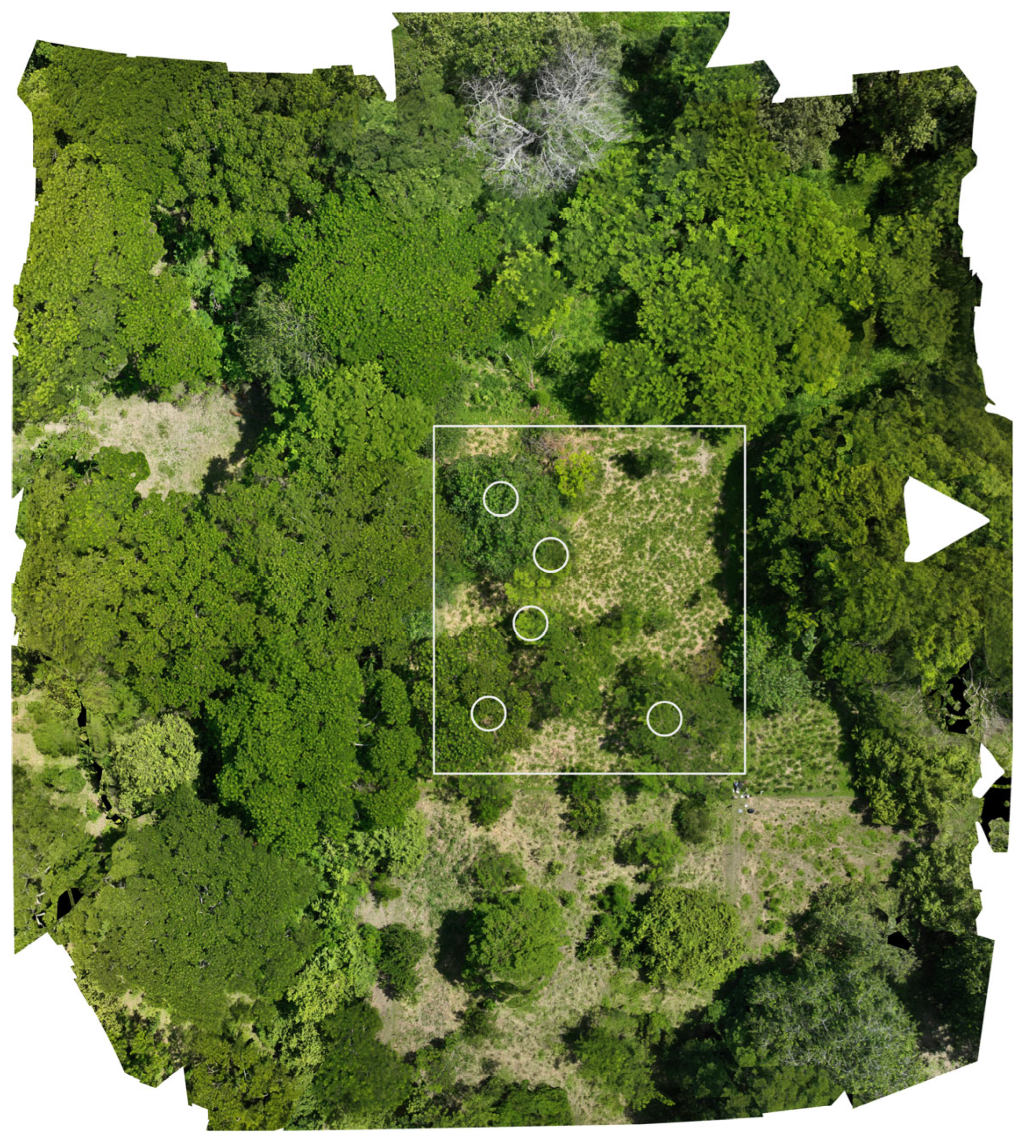
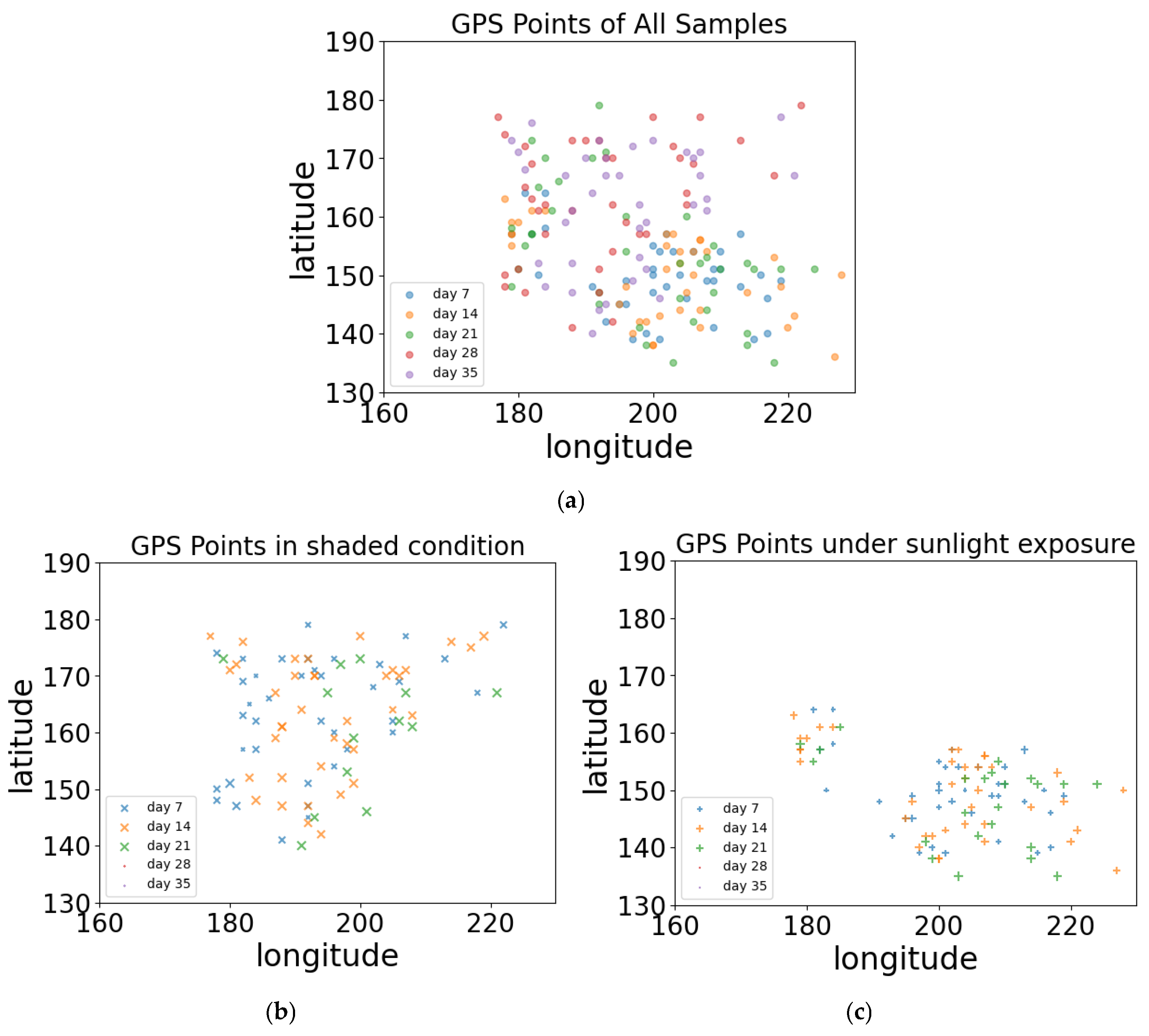
3.1.1. Experimental Design and Sampling Location

A 35-day experiment was conducted to evaluate the growth of Megathyrsus maximus cv. Mombasa using handheld VIS-NIR optical spectrometer and RGB cameras in a plot within the Sustainable Beef Production Model (SBPM) at the Turipaná Research Centre of Corporacion Colombiana de Investigación Agropecuaria—AGROSAVIA, situated in the Caribbean region of Colombia in the municipality of Cereté, in the department of Córdoba. The global coordinates for SBPM are as follows: 8°50′33.9″ N, 75°48′6.5″ W; 8°50′33.6″ N, 75°48′0.1″ W; 8°50′30.2″ N, 75°48′3.3″ W; and 8°50′30.3″ N, 75°48′6.5″ W. The SBPM area has an average annual precipitation of 1646 mm and a maximum daily precipitation of 137 mm. The average relative humidity is 80.1%, ranging from 76% to 83%, according to data from the Turipaná climatological station. The average daily temperature is 28 °C. The agroecological zone is classified as tropical dry forest.

The SBPM consists of a silvopastoral arrangement with scattered trees divided into eight paddocks. For this experiment, one paddock has an area of 0.27 ha (2700 m²), where a count of 100 m² recorded 283 tussocks, allowing an estimation of approximately 7641 tussocks in the entire area (see Figure 1). It was selected under an intensive rotational grazing system, where trees have naturally regenerated within the paddocks [14].

The sampling geolocation followed the pattern in Figure 2, ensuring representative coverage during the five sessions. Strategically positioned points captured field variability, targeting “twin” tussocks to optimize biomass and forage quality assessment. Latitude and longitude geolocations per tussock were collected using digital GPS reference GARMIN GPSmap 62s.

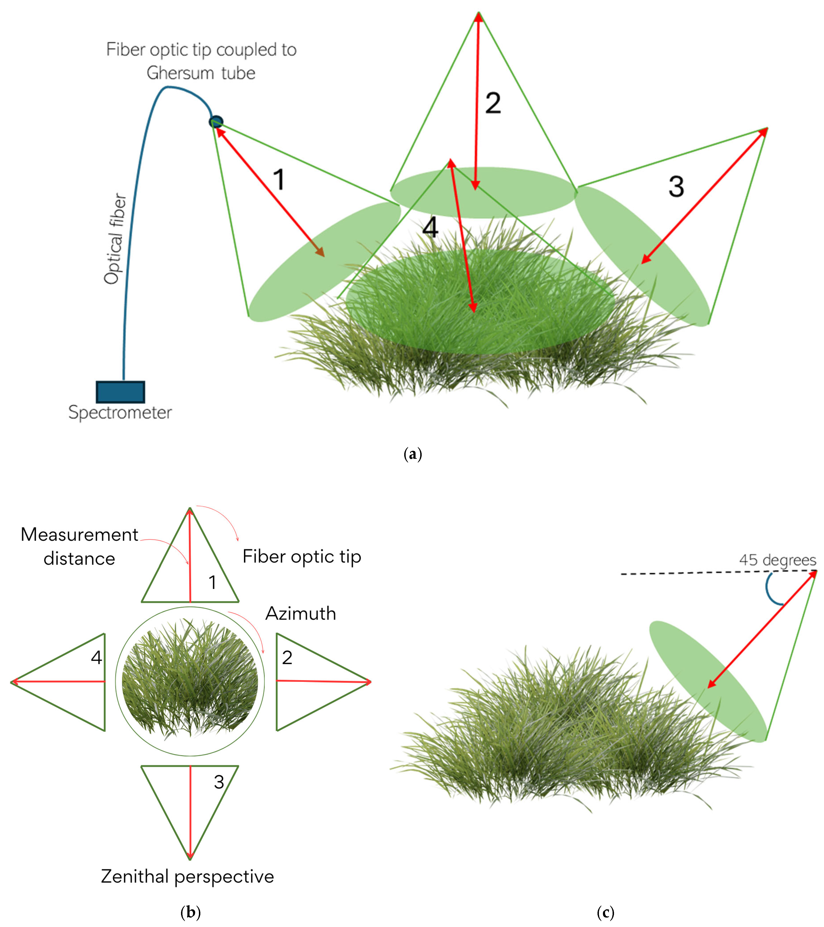
3.1.2. Forage Sampling Method

A trained worker performed the homogenization cut of the pasture at a height of 30 cm above the ground using an electric scythe, measuring the height with a ruler. Several tussocks were randomly measured to verify the height. Evenly spaced regrowth measurements were carried out five times from day 7 to day 35, between 7:00 A.M. and 11:00 A.M. during a rainy period from 16 August to 16 September 2024. Meteorological data from the five sessions were collected from The IDEAM Meteorological Station of Turipaná Research Center of AGROSAVIA, located in Cereté Córdoba, Colombia, with the official code 13075060. The records included environmental parameters such as precipitation, ambient temperature, and solar radiation. Meteorological data for the five experimental sessions are shown in

Table 1. Meteorological data collected during the five sampling days.

Regrowth Day	Relative Humidity (%)	Solar Radiation	Precipitation (mm)	Air Temperature
7	67.3	21.1	7.4	30.5
14	70.3	23.5	46.7	29.1
21	75.7	10.6	0.0	28.8
28	71.3	2.7	13.3	29.4
35	72.0	2.8	0.0	28.7

.

Regarding forage sampling, forty (40) Mombasa grass tussocks (19 under shade, 21 under sunlight) were selected in each session, corresponding to different ages of regrowth: 7, 14, 21, 28, and 35 days. This sample size (40 tussocks per day) is statistically representative, as the required sample size, calculated with a 95% confidence level and 15% margin of error, was 42 tussocks, which is very close to the one used in the study. An effort was made to select a ’twin’ tussock in each session, matching the one sampled previously. This approach resulted in a total of 200 tussocks sampled throughout the experiment.

3.1.3. Forage Evaluation

Initially, each grass tussock was characterized by measuring its height, the number of total green leaves, green leaves per stem, and dry matter yield (DMY).

• Height per tussock: This is measured in cm from the ground to the apical leaf (without compressing or extending it), excluding the inflorescence. A tape measure with a resolution of 0.1 cm was used.
• Green leaves per stem: To estimate the number of green leaves per stem, 20% of the total stems in the tussock were sampled. The green leaves on each stem were counted, from the basal leaf to the apical leaf, and the mode of the values of the sample was recorded.
• Number of total green leaves per tussock: The total number of green leaves was manually counted.
• Biomass per tussock (DMY): A cut was made at a height of 30 cm using an electric hedge trimmer. The material was collected, and its fresh weight was measured in situ using a digital scale with a resolution of 0.1 g. Subsequently, a 250 g subsample was taken and dried in an oven at 65 °C for 48 h to calculate the dry matter based on the difference between the fresh and dry weights of the samples. The dry weight of the tussock was then calculated by multiplying its fresh weight by its dry matter concentration.

Additionally, visible RGB images per tussock were taken using a Samsung S23 camera smartphone of 50MP (S5KGN3 1/1.57″ sensor with 1.0 µm pixels and a Tetracell filter). The photo was taken parallel to the tussock, capturing the entire plant from its base to its apex with a field of view of 123°. Four spectra were collected using an Ocean Insight VIS-NIR spectrometer (SR-4VN500-5) operating at (350–1100 nm) to obtain the spectral signatures. Before measurement, radiometric calibration was an essential step to ensure accurate and repeatable results. For this purpose, a Lambertian reference white was used, which is a material with uniform diffuse reflectance in all directions, minimizing angular effects and variations in illumination. A Spectralon panel, widely used for its high stability and well-characterized reflectance over a broad spectral range, was employed, followed by measurement of background radiation to establish the maximum and minimum reflectance values under the experimental lighting conditions. The implementation of this procedure allowed for the calibration of the spectrometer measurements and ensured the reliability of the data in this study.

Regarding spectral signatures, they were recorded at four azimuthal positions using the VIS-NIR spectrometer coupled with Ghersum tubes (1°, 3°, 8°, and 14°). These tubes adjusted the angular optical field of view, improving the signal-to-noise ratio, especially in wavelengths with low reflectance due to variations in the optical receiver’s sensitivity. Measurements were taken at a zenith angle of 45°, isolating plant canopy radiation and minimizing soil interference as proposed in [12,25]. The recording distance, ranging from 7.5 to 80 cm based on the Ghersum tube used, was calculated using geometric optics to target the reflection area (Figure 3).

3.1.4. Bromatological Analysis

A representative sampling of the areas under study was carried out separately for quality analysis, from which two subsamples of 500 g each were taken. The first subsample was obtained from the pasture exposed directly to sunlight, while the second subsample was taken from the pasture located beneath the trees in the paddock. Both subsamples were collected using the “hand plucking” methodology described by Cook [26]. Subsamples were dried in an air oven at 65 °C for 48 h and grounded with a 2 mm sieve [27]. Bromatological analysis was performed using wet chemistry to determine relevant nutritional parameters of the pasture, such as crude fiber (CP), neutral detergent fiber (NDF), acid detergent fiber (ADF), lignin content (LIG), crude protein (CP), ether extract (EE), and ash (ASH), using the AOAC methods [16]. The procedures were carried out in the analytical chemistry laboratory of the Turipaná Research Center.

3.2. In-Field Database Analysis

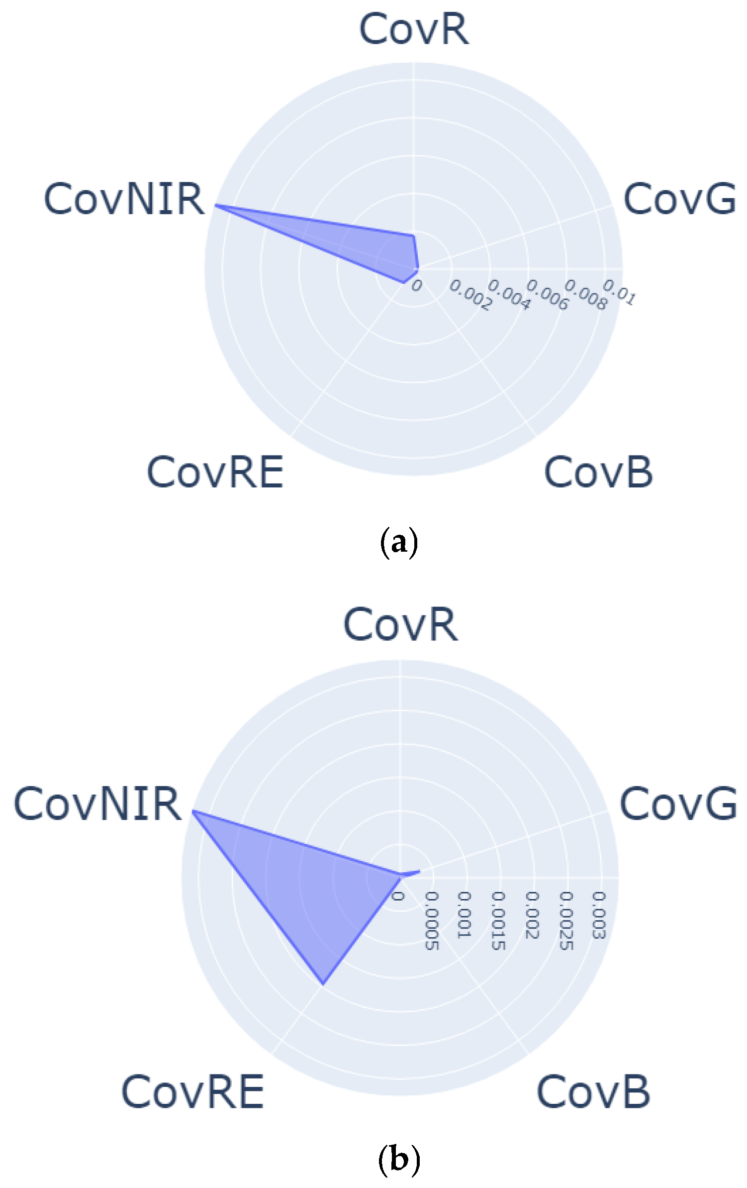
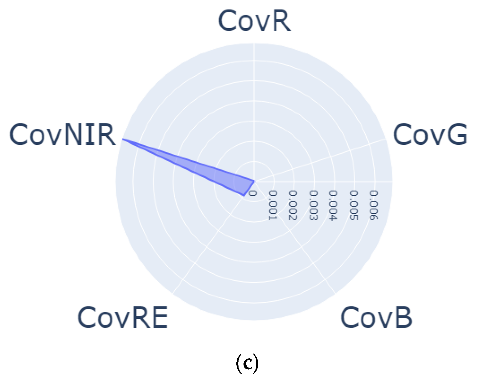
3.2.1. Data Engineering of VIS-NIR Optical Spectra, Segmentation of Visible RGB Images, and Implementation of Covariance Strategies

For optical spectrum processing, a Python 3.1.1.9 script was developed to compute the most relevant features from VIS-NIR optical wavelengths using the reflectance spectra captured. Reflectance at specific wavelengths, including near-infrared (NIR, 850 nm), red edge (RE, 780 nm), green (G, 560 nm), blue (B, 450 nm), and red (R, 650 nm), were extracted from the spectra. Further, 24 vegetation indices (

Table 2. Vegetation indices extracted from VIS-NIR optical spectrum.

Name of Vegetation Index	Equation
Normalized Vegetation Difference Index (NDVI)	$NDVI={\displaystyle \frac{\left(R_{NIR}-R_R\right)}{\left(R_{NIR}+R_R\right)}}$
Green Normalized Difference Vegetation Index (GNDVI)	$GNDVI={\displaystyle \frac{\left(R_{NIR}-R_G\right)}{\left(R_{NIR}+R_G\right)}}$
Normalized Difference Vegetation Red Edge (NDRE)	$NDRE={\displaystyle \frac{\left(R_{NIR}-R_{RE}\right)}{\left(R_{NIR}+R_{RE}\right)}}$
Plant Senescence Reflectance Index (PSRI)	$PSRI={\displaystyle \frac{\left(R_R-R_G\right)}{R_{RE}}}$
Triangular Vegetation Index (TVI)	$TVI=0.5\times 120\left(R_{RE}-R_R\right)-200\left(R_R-R_{\left(B\right)}\right)$
Soil Adjusted Vegetation Index (SAVI)	$SAVI={\displaystyle \frac{1.5\times \left(R_{NIR}-R_R\right)}{\left(R_{NIR}+R_R+0.5\right)}}$
Optimized Soil Adjusted Vegetation Index (OSAVI)	$OSAVI={\displaystyle \frac{R_{NIR}-R_R}{\left(R_{NIR}+R_R+0.16\right)}}$
Atmospherically Resistant Vegetation Index (ARVI)	$ARVI={\displaystyle \frac{R_{NIR}-R_{R-B}}{\left(R_{NIR}+R_{R-B}\right)}}$ $R_{R-B}=R_R-\gamma \left(R_R-R_B\right)$ $\gamma =1$
Soil Adjusted and Atmospherically Resistant Vegetation Index (SARVI)	$SARVI={\displaystyle \frac{2\times \left(R_{NIR}-R_{R-B}\right)}{\left(R_{NIR}+R_{R-B}+1\right)}}$
Soil Adjusted and Atmospherically Resistant Vegetation Index 2 or Enhanced Vegetation Index (SARVI2 o EVI)	$EVI={\displaystyle \frac{2G\times \left(R_{NIR}-R_R\right)}{\left(R_{NIR}+C_1\times R_R-C_2\times R_R+1\right)}}$ $G=2.5,C_1=6,C_2=7,5yL=1$
Enhanced Vegetation Index 2 (EVI2)	$EVI2={\displaystyle \frac{2.5\times \left(R_{NIR}-R_R\right)}{\left(R_{NIR}+2.4\times R_R+1\right)}}$
Non-Linear Vegetation Index (NLI)	$NLI={\displaystyle \frac{\left(R_{NIR}^2-R_R\right)}{\left(R_{NIR}^2+R_R\right)}}$
Visible Atmospherically Resistant Index (VARI)	$VARI={\displaystyle \frac{\left(R_G-R_R\right)}{\left(R_G+R_R-R_{NIR}\right)}}$
Chlorophyll Index Green (CLGR)	$CLGR={\displaystyle \frac{R_{NIR}}{R_G}}-1$
Chlorophyll Index Red Edge (CLRE)	$CLRE={\displaystyle \frac{R_{NIR}}{R_{RE}}}-1$
Normalized Difference Vegetation Water Index (NDWI)	$NDWI={\displaystyle \frac{R_G-R_{NIR}}{R_G+R_{NIR}}}$
Renormalized Difference Vegetation Index (RDVI)	$RDWI={\displaystyle \frac{R_G-R_{NIR}}{{\left(R_G-R_{NIR}\right)}^{\frac{1}{2}}}}$
Renormalized Difference Vegetation Index (WDRVI)	$WDRWI={\displaystyle \frac{0.1R_{NIR}-R_R}{0.1R_{NIR}+R_R}}$
Leaf Area Index (LAI)	$LAI=3.618EVI-0.118$
Anthocyanin Reflectance Index 1 (ARI1)	$AR{I}_1={\displaystyle \frac{1}{R_G}}-{\displaystyle \frac{1}{R_{RE}}}$
Anthocyanin Reflectance Index 2 (ARI2)	$AR{I}_2=R_{NIR}\times \left({\displaystyle \frac{1}{R_G}}-{\displaystyle \frac{1}{R_{RE}}}\right)$
Blue Green Pigment Index (BGI)	$BGI={\displaystyle \frac{R_B}{R_G}}$
Normalized Phaeophytinization Index (NPQI)	$NPQI={\displaystyle \frac{R_R-R_B}{R_R+R_B}}$
Plant Senescence Reflectance Index (PSRI)	$NSRI={\displaystyle \frac{R_R-R_G}{R_{RE}}}$
Structure Insensitive Pigment Index 1 (SIPI1)	$SIPI={\displaystyle \frac{R_{NIR}-R_B}{R_{NIR}+R_G}}$

R is the reflectance, and R_x is the reflectance at a specific wavelength x given by (NIR, 850 nm), red edge (RE, 780 nm), green (G, 560 nm), blue (B, 450 nm), and red (R, 650 nm).

) related to production biomass and forage quality traits were calculated [24].

Regarding image processing, segmentation of visible RGB images using Mahalanobis distance to assess green variability in pasture growth was implemented. Visible RGB images were captured using a consumer-grade smartphone (Samsung 50MP). Precise segmentation of green regions in RGB images remains challenging due to overlapping colors and varying lighting conditions, which reduce the accuracy of digital filtering techniques [28]. However, the application of Mahalanobis distance improves segmentation accuracy by considering the statistical variability of colors. Segmentation results were used to characterize greenness intensity and variance associated with the evolution of green tones and pixel counts during different stages of pasture growth. Image processing using the Mahalanobis distance was implemented in three steps with a Python script. First, the RGB channels were normalized to minimize the influence of illumination variability caused by environmental changes. Second, a set of training data representing green values was manually defined. Third, the mean µ covariance matrix Σ of the green class (pixel selected) was calculated. The Mahalanobis distance for each pixel was computed as follows:

$$D^2={\left(x-\mu \right)}^T{\mathsf{\Sigma }}^{-1}\left(x-\mu \right)$$

(1)

where x is the RGB vector of the pixel and Σ⁻¹ is the inverse covariance matrix. Pixels with distances below a defined threshold are classified as green [29,30].

As a proposal of data engineering to introduce categorical variables, covariance values were calculated to characterize the non-uniformity of the tussock, as observed in differences in the NIR values from the four recorded spectra. Additionally, greenness—defined as the difference between the mean green pixel values and the segmented green pixel values obtained using the Mahalanobis distance segmentation method—was incorporated. These factors were used to create a categorical variable named ’non-uniformity’, which was added to the dataset to account for both NIR variation (derived from the covariance values) and green variability in the tussock. This approach is aimed at enhancing the performance of machine learning models in predicting biomass and pasture quality.

Finally, the data recorded in the field, the processed data (spectra and images), and the data obtained in the laboratory were compiled into an Excel 2503 file (see Supplementary Materials) database for management using Python’s Pandas library. The data types are described in

Table 3. Descriptions of experimental data variables that conform to the database.

Data Source	Database Parameters
Data recorded in-field	Date Regrowth day Tussock location: Whether it is in the shade or under the sun Number of tussocks (from 0–39) Geolocation recorded by GPS Tussock’s variables: Height Number of total green leaves Green leaves per stem One (1) photo per tussock and four (4) spectra Biomass per tussock: Fresh weight and subsamples
Laboratory data	Percent of dry matter (%) gr of dry matter per tussock Quality variables: Crude fiber (CF), neutral detergent fiber (NDF), acid detergent fiber (ADF), lignin content (LIG), crude protein (CP), ether extract (EE), ash (ASH)
Data processed	Optical VIS-NIR spectrum values: Optical reflectance of NIR, B, G, RE, R, and vegetation indices (Table 2) NIR covariance, mean green values, pixel numbers, and greenness p Categorical variable: Non-uniformity derived through thresholding classification of covariance values and greenness values

.

3.2.2. Machine Learning Model Description

Machine learning (ML) models were used to predict the biomass and forage quality of Mombasa grass based on environmental and optical parameters to support livestock management. A Python script utilizing Sk-learn, Pandas, Numpy, and Statsmodels libraries was developed to evaluate the performance of conventional linear regression (LR), LASSO, Ridge, ElasticNet, k-nearest neighbors (K-NN), and decision tree models for prediction. Five steps were implemented: (1) data preprocessing, (2) training, (3) model evaluation, (4) validation, and (5) testing [31]. Initial data preprocessing included scaling and normalizing numerical variables and encoding categorical variables. Further, linear dependencies between variables were evaluated using Pearson’s correlation matrix.

The dataset, consisting of 200 samples, was split into 80% for training (160 samples) and 20% for testing (40 samples) for model training and validation. Linear regression using ordinary least squares (OLS) R² and MAE were implemented to identify patterns and minimize prediction errors.

Cross-validation with 42 random training and testing data subsets was performed to assess the performance of models, reducing the variance and preventing overfitting. The assumptions of linear regression, including linearity, independence, homoscedasticity, and normality of residuals, were thoroughly assessed.

Hyperparameter tuning using grid search and cross-validation was applied to ML models such as LASSO, Ridge, ElasticNet, and k-NN to optimize model parameters for both biomass and quality traits, ensuring reliable performance. The hyperparameter α is used in LASSO, Ridge, and ElasticNet, where it controls the strength of the regularization based on the L1 (LASSO) and L2 (Ridge) cost functions, adjusting for better performance. The number of neighbors (N) is the key hyperparameter in k-NN regression, representing the number of neighbors considered for adjusting the regression line. In decision trees, the maximum number of features (MF) and maximum depth (MD) are the primary hyperparameters that influence model complexity and performance. Simple LR does not have hyperparameters. The optimized hyperparameter values are presented in

Table 4. Hyperparameter tunning results applied to ML models. EN: ElasticNet, DT: Decision Tree, N: the number of neighbors, MF: maximum number of features, MD: maximum depth.

Adjusted Hyperparameters for Biomass and Quality Trait Prediction
Under Shaded Conditions
ML Model	g of Dry Matter				CF				NDF				ADF
	α	N	MD	MF	α	N	MD	MF	α	N	MD	MF	α	N	MD	MF
LASSO	1.0				0.2				1.0				0.8
EN	1.0				0.2				1.0				0.8
Ridge	1.0				0.2				1.0				0.8
k-NN		25				10				50				35
DT			7	20			4	30			9	20			4	30
ML model	LIG				CP				EE				ASH
	α	N	MD	MF	α	N	MD	MF	α	N	MD	MF	α	N	MD	MF
LR
LASSO	0.2				0.2				0.2				0.2
EN	0.2				0.2				0.2				0.2
Ridge	0.2				0.2				0.2				0.2
k-NN		50				50				50				25
DT			5	30			9	30			4	30			9	30
Under Sunlight Exposure
ML model	g of dry matter				CF				NDF				ADF
	α	N	MD	MF	α	N	MD	MF	α	N	MD	MF	α	N	MD	MF
LASSO	1.0				1.0				0.2				1.0
EN	1.0				1.0				0.2				1.0
Ridge	1.0				1.0				0.2				1.0
k-NN		12				10				10				10
DT			5	30			7	30			7	30			5	30
ML model	LIG				CP				EE				ASH
	α	N	MD	MF	α	N	MD	MF	α	N	MD	MF	α	N	MD	MF
LASSO	0.2				0.2				0.2				0.2
EN	0.2				0.2				0.2				0.2
Ridge	0.2				0.2				0.2				0.2
k-NN		10				10				10				10
DT			5	20			4	30			5	10			9	30

.

Regarding linear regression models, in LASSO, an α value of 1 applies a moderate L1 regularization, potentially setting some coefficients to zero. In Ridge, it represents a moderate L2 penalty, shrinking coefficients without eliminating them. In Elastic Net, if the L1 ratio (hyperparameter of ElasticNet) = 1, the model behaves like LASSO.

For α = 0.8, LASSO applies a moderate L1 regularization, reducing some coefficients to zero but less aggressively than when α = 1. In Ridge, it represents an intermediate L2 penalty, shrinking the magnitude of the coefficients without eliminating them. In Elastic Net, if the L1 ratio = 0.8, the model applies 80% L1 regularization and 20% L2 regularization, combining features of both methods.

For α = 0.2, LASSO applies a mild L1 regularization, meaning fewer coefficients will be reduced to zero compared to higher α values. In Ridge, it represents a low L2 penalty, allowing greater flexibility in the coefficients. In Elastic Net, if the L1 ratio = 0.2, the model applies 20% L1 regularization and 80% L2 regularization, prioritizing the reduction of coefficient magnitudes without eliminating them.

In a k-NN (k-Nearest Neighbor) model, choosing several neighbors (k) between 10 and 50 helps smooth predictions, reducing the risk of overfitting. As k increases, the model becomes more general and less sensitive to noise or outliers, improving stability; however, higher values (closer to 50) may cause underfitting by losing important local patterns. Additionally, a larger k increases computational complexity, as more distances need to be calculated. Overall, selecting k in this range provides a balance between robustness and detail, making it suitable for datasets requiring stable predictions.

In the decision-tree-based models, the maximum number of features (MF: 20–30) defines how many features are considered for each split, ensuring a balance between diversity and accuracy. A range of 20–30 means the model selects the best split from this subset rather than using all features, which can improve performance in ensemble methods. The maximum depth (MD: 4–7) limits the tree’s complexity, preventing overfitting while capturing key patterns. A shallower tree (MD = 4) generalizes better but may underfit, whereas a deeper tree (MD = 7) captures more complexity but risks overfitting. This configuration provides a trade-off between model interpretability and predictive power.

Following training, each model was evaluated using performance metrics like accuracy, R², and MAE to assess how well the model generalized to testing datasets, where R² is useful for evaluating the overall fit of the model while MAE measures the accuracy of predictions in the same units as the target variable.

Permutation importance was applied to identify the most influential features by permuting their values and observing the resulting impact on model accuracy. Features with low importance were removed from the analysis and further adjustments were made, including modifying features or tuning hyperparameters, and the models were re-validated. Finally, the model was tested on a separate dataset, distinct from the training and validation sets, to assess its performance in real-world scenarios and confirm its ability to generalize unseen data. As the data exhibits high multicollinearity, the Ridge ML model is the best-suited approach for adjusting the prediction model, solving multicollinearity in regression analysis. Multicollinearity occurs when two or more explanatory variables are highly correlated with each other. The theoretical foundations are presented as follows.

Ridge regression is a regularized linear regression method that addresses multicollinearity and overfitting by incorporating an L2 regularization term in the loss function. This additional term penalizes large coefficient values, ensuring that the model remains stable even when predictor variables are highly correlated [32].

In ordinary least squares (OLS) regression, the objective is to minimize the residual sum of squares (RSS):

$$RSS={\sum }_{i=1}^n{\left(y_i-\dot{y_i}\right)}^2$$

(2)

where $y_i$ is the actual response variable, $\dot{y_i}$ is the predicted response, and n is the number of observations. However, when predictor variables exhibit high collinearity, OLS coefficients become unstable and may have a large variance. To mitigate this, Ridge regression modifies the cost function by adding an L2 penalty term:

$$RS{S}_{Ridge}={\sum }_{i=1}^n{\left(y_i-\dot{y_i}\right)}^2+\lambda {\sum }_{j=1}^p{\beta }_j^2$$

(3)

where $\lambda$ is the regularization parameter that controls the strength of the penalty, ${\beta }_j$ are the regression coefficients, and p is the number of predictors.

By shrinking the coefficient towards zero, Ridge regression reduces model complexity while maintaining predictive power, especially when dealing with noisy or correlated input features. L2 regularizations work by adjusting $\lambda$ values, preventing excessive variance due to multicollinearity. If predictor variables are highly correlated, Ridge regression helps stabilize the model by distributing the coefficient weights more evenly. Additionally, it reduces overfitting by penalizing large coefficients, thereby improving generalization to new data. Moreover, Ridge introduces a small bias, leading to more robust predictions.

In the context of forage quality prediction, the dataset includes multiple spectral features extracted from images and spectrometers, as well as visual variables such as height and the number of leaves, which can be highly correlated. Ridge regression helps mitigate multicollinearity via the following:

• Ensuring that correlated spectral variables do not distort coefficient estimates.
• Preventing overfitting, especially when working with high dimensional datasets, as seen in spectral analysis.
• Improving generalization by allowing the model to perform better on unseen data by reducing variance.

By leveraging Ridge regression, this study ensures robust and generalizable predictions of forage quality, even in complex environments like silvopastoral systems.

4. Results

4.1. In-Field Dataset Configuration and Visualization

4.1.1. Forage Sampling Results

In terms of the characterization of variables measured in the tussock, the results of the forage evaluation showed that for the numerical observation of total green leaves per tussock, no differences were evident in the phenological development of the plant until day 21 of growth. Starting from day 28, numerical differences were observed between the tussocks under shade and those in the sun for both variables, with greater development observed in the tussocks exposed to the sun because of direct radiation, which enhances the plant’s photosynthetic capacity and promotes vigorous development. On day seven (7), differences in total green leaves between tussocks in shade and sunlight were likely caused by selection bias during the initial session, which resulted in non-representative samples from the shaded environment.

The number of leaves per stem remained the same regardless of the location of the tussock, showing that the phenological development of the plant is influenced by age rather than radiation conditions. However, leaf elongation is directly related to the location of the tussocks and the interception of sunlight. This is reflected in the greater height of the tussock exposed to sunlight and explains the higher accumulation of dry matter (see

Table 5. Descriptive statistics of measured variables for each tussock throughout the experiment.

Regrowth Day	Tussock’s Location	No. of Green Leaves per Stem	No. of Green Leaves per Tussock		Height’s Tussock (cm)		DMY per Tussock (g)
		Mode	Mean	S.D.	Mean	S.D.	Mean	S.D.
7	Shaded	2	72	19.64	66.26	8.41	15.19	6.41
	Sunlight	2	105	36.79	67.33	6.87	21.12	7.75
14	Shaded	3	183	45.15	81.00	9.49	41.05	13.78
	Sunlight	3	185	45.18	78.67	9.29	48.72	18.81
21	Shaded	4	192	49.41	100.53	10.82	62.82	20.09
	Sunlight	4	192	52.93	108.71	7.05	75.42	21.17
28	Shaded	4	215	80.46	122.11	12.62	98.18	44.08
	Sunlight	4	244	61.53	130.14	6.44	123.94	27.01
35	Shaded	5	331	76.31	136.84	10.55	136.66	35.66
	Sunlight	5	356	74.52	151.71	9.18	169.12	40.29

S.D.: standard deviation.

).

4.1.2. Bromatology Quality Results

As expected, the nutritional quality of Mombasa grass for the different regrowth days showed an increase in fiber components (CF, NDF, ADF, and LIG) with pasture age. These variables are directly related to the potential intake and digestibility of the pasture, and their measurement is useful for decision making about the time of animal access to pasture.

On the other hand, the accumulation of fibers in the tussocks leads to a gradual decrease in EE and CP components, thus reducing the nutritional value of the forage as the plant matures (see

Table 6. Nutritional composition (%) of Mombasa grass across different regrowth days.

Regrowth Day	Tussock’s Location	CF	NDF	ADF	LIG	CP	EE	ASH
7	Shaded	29.40	58.11	32.85	6.68	18.19	2.48	12.51
	Sunlight	29.61	57.27	32.21	8.93	18.09	2.32	12.78
14	Shaded	29.59	59.29	32.90	8.46	17.10	2.59	11.89
	Sunlight	30.47	59.81	33.19	2.39	14.44	2.48	12.55
21	Shaded	32.14	60.04	36.12	6.11	15.69	2.30	12.24
	Sunlight	33.99	62.25	38.62	3.18	11.59	2.66	13.30
28	Shaded	35.63	62.42	38.79	3.45	12.00	1.91	11.78
	Sunlight	34.92	62.53	39.00	3.19	9.37	1.74	11.39
35	Shaded	34.90	62.92	38.69	4.96	15.21	1.78	12.05
	Sunlight	35.63	63.36	40.56	3.65	9.75	1.78	12.27

). The variability observed in the nutritional components of the plant under sunlight or shaded became a challenge in animal management in the herd; therefore, this scenario was suitable for evaluating the capability of remote sensing and modeling.

4.2. Final Database Configuration

Data Engineering

Figure 4 shows the four unprocessed spectra taken from a tussock (tussock labeled No. 18) during the experiment. The observed NIR variation ranged from 50% to 100%, emphasizing the importance of quantifying this variation through covariance values to enhance the predictive performance of the ML model. These four spectra were captured for each of the 40 tussocks during the five sessions, resulting in 800 spectra. A Python code was executed to process spectra by using computational filters to compute optical reflectance at wavelengths in the NIR (850 nm), RE (780 nm), G (560 nm), blue (B, 450 nm), and red (R, 650 nm), as well as 24 vegetation indices to be incorporated in the final database.

Figure 5 illustrates the results following the steps to process the images using the Mahalanobis distance segmentation method. In this experiment, images were processed from each of the 40 tussocks across the five sessions, resulting in a total of 200 images. The Mahalanobis distance was used to segment the images by evaluating how far each green pixel deviated from a reference distribution [30]. This reference (Figure 5a) was constructed by manually extracting 10 to 100 pixels from the target class, accounting for the correlations among the RGB channels. These features were then analyzed to determine the distribution of each object class in the image (e.g., tussocks, background, or other objects of interest), ultimately extracting the tussock pixels.

Pixels that exhibited lower Mahalanobis distance to the reference class enable precise segmentation and extraction of the green tussock pixels [30].

Covariance results were computed by analyzing the differences between NIR reflectance and other optical reflectance wavelengths. Figure 6 presents covariance values across various regrowth days for three randomly selected tussocks using a radar diagram. It also illustrates the covariance variation at different wavelengths (R, G, B, RE, NIR), with NIR covariance being significantly higher—by up to three orders of magnitude—compared to the others.

The integration of NIR covariance and green variation into a single variable, ’non-uniformity’, was a key factor for inclusion in the ML model.

4.3. Development and Analysis of Machine Learning Models

First, Pearson correlation analysis revealed strong correlations with optical parameters from 0.5 to 0.98, with p-values less than 0.05 supporting the use of linear regression for predicting biomass and quality traits. Cross-validation showed that Ridge outperformed predictions of biomass and quality traits, followed by the decision tree, whereas the K-NN regressor performed the worst (see

Table 7. Biomass and quality trait R² metrics of applied ML models. TR: Training (training Score), T: test (test score), EN: ElasticNet, DT: Decision Tree.

Biomass and Quality Traits
Under Shaded Conditions
ML Model	g of Dry Matter		CF		NDF		ADF		LIG		CP		EE		ASH
	TR	T	TR	T	TR	T	TR	T	TR	T	TR	T	TR	T	TR	T
LR	0.953	0.353
LASSO	0.903	0.865	0.918	0.843	0.844	0.864	0.841	0.826	0.723	0.642	0.889	0.915	0.809	0.797	0.342	0.368
EN	0.901	0.886	0.840	0.687	0.846	0.868	0.844	0.825	0.821	0.803	0.848	0.880	0.819	0.802	0.387	0.391
Ridge	0.913	0.815	0.999	0.998	0.985	0.953	0.989	0.966	0.998	0.996	0.998	0.996	0.998	0.993	0.999	0.997
k-NN	0.139	−0.158	0.334	−0.185	0.068	−0.075	0.105	−0.033	0.011	−0.025	0.021	0.021	0.041	−0.116	0.085	0.078
DT	0.999	0.786	0.999	0.999	0.999	0.999	0.999	0.999	0.999	0.999	0.999	0.999	0.999	0.999	0.999	0.999
Under Sunlight Exposure
LR	0.954	0.529
LASSO	0.924	0.934	0.906	0.881	0.910	0.810	0.898	0.879	0.836	0.701	0.899	0.904	0.771	0.786	0.521	0.591
EN	0.924	0.933	0.910	0.890	0.911	0.811	0.902	0.887	0.825	0.648	0.921	0.840	0.773	0.781	0.571	0.622
Ridge	0.934	0.902	0.986	0.969	0.998	0.994	0.986	0.969	0.999	0.997	0.998	0.995	0.998	0.996	0.999	0.998
k-NN	0.162	−0.253	0.179	0.274	0.246	−0.193	0.180	−0.239	0.462	−0.243	0.230	−0.270	0.432	−0.290	0.466	0.063
DT	0.979	0.929	0.999	0.999	0.999	0.999	0.999	0.999	0.999	0.999	0.999	0.999	0.999	0.798	0.999	0.999

The higher R² values, indicating the best-adjusted ML model, are in bold.

). Performance was assessed using the key evaluation metric R² as an indicator of model efficiency. As more information is incorporated, accuracy improves. However, due to the interaction of biological organisms with the environment, increasing the sample size contributes to greater precision. While R² reflects the explanatory power of the model, MAE provides a more tangible measure of error. In models where data dispersion is high or the relationship is not strictly linear, MAE can be a more reliable metric for assessing accuracy. Both metrics are presented here.

The two best-adjusted models, identified in bold text, were determined by analyzing both the training and test scores and comparing them to the other models. The slight decrease in the test R² compared to the training R² suggests that the model generalizes well, with only minor overfitting. This behavior is observed by reliable models that generalize effectively unseen data, highlighting its predictive accuracy and stability. The LR model was not used for quality prediction due to a lack of multicollinearity issues.

The two best-adjusted models, highlighted in bold, were selected by analyzing both the training and test scores and comparing them to the other models. The low values and slight difference in test MAE compared to training MAE suggest a very low error in the best-chosen model relative to the R² metric, as shown in

Table 8. Biomass and quality trait MAE metrics of applied ML models. TR: Training (training Score), T: test (test score), EN: ElasticNet, DT: Decision Tree.

Biomass and Quality Traits
Under Shaded Conditions
ML Model	g of Dry Matter		CF		NDF		ADF		LIG		CP		EE		ASH
	TR	T	TR	T	TR	T	TR	T	TR	T	TR	T	TR	T	TR	T
LR	8.51	23.69
LASSO	10.77	11.98	0.71	0.62	0.55	0.49	0.81	0.77	0.72	0.64	0.55	0.47	0.11	0.09	0.18	0.19
EN	10.80	11.03	1.00	1.23	0.56	0.49	0.80	0.77	0.59	0.51	0.64	0.54	0.10	0.09	0.17	0.18
Ridge	10.62	13.76	0.05	0.08	0.17	0.26	0.21	0.33	0.04	0.06	0.05	0.09	0.01	0.01	0.006	0.01
k-NN	40.35	35.75	2.08	2.24	1.71	1.66	2.33	2.2	1.43	1.13	1.64	1.56	0.30	0.26	0.20	0.22
DT	6.04	10.31	0.0	0.0	0.0	0.0	0.0	0.0	0.0	0.0	0.0	0.0	0.0	0.0	0.0	0.0
Under Sunlight Exposure
LR	9.39	31.03
LASSO	12.15	12.78	0.60	0.75	0.52	0.85	0.82	1.06	0.74	1.12	0.83	1.30	0.14	0.15	0.39	0.31
EN	12.26	12.86	0.58	0.72	0.52	0.85	0.81	1.03	0.75	1.20	0.73	1.17	0.13	0.15	0.36	0.30
Ridge	11.34	14.92	0.22	0.39	0.07	0.15	0.30	0.53	0.05	0.11	0.11	0.21	0.01	0.01	0.01	0.02
k-NN	43.08	56.00	1.88	2.56	1.57	2.20	2.60	3.48	1.16	1.91	2.30	3.30	0.23	0.34	0.37	0.49
DT	0.02	15.89	0.0	0.0	0.0	0.0	0.0	0.0	0.0	0.0	0.0	0.0	0.0	0.03	0.0	0.0

The lower MAE values, indicating the best-adjusted ML model, are in bold.

.

The Ridge model maintains good accuracy in both conditions (shade and sunlight), suggesting that it can adapt to changes in the environment and its capability for accurate biomass production and nutritional quality prediction (see Table 7 and Table 8). The model was shown to fit well in both datasets, suggesting that its predictions in new environmental conditions would be reliable.

A high R², as obtained here, indicates that the model can estimate the quantity and quality of available pasture with greater confidence, allowing producers to make more informed decisions regarding livestock rotation, fertilization, and harvest planning. This further justifies the use of more precise technologies, such as those explored in this study, based on proximal and handheld sensors.

If the model had a low R², the prediction of forage biomass and quality would have been less reliable, potentially leading to inefficient pasture management, affecting livestock feed availability and, consequently, their productive performance. Increasing sample size and considering the representation of the system’s environmental and biological conditions can help enhance model accuracy, enabling more efficient and sustainable pasture management.

4.3.1. Prediction of Biomass Based on Dry Matter Yield

Based on cross-validation, the ElasticNet and LASSO models demonstrated the best fit among the models tested for predicting biomass. The ElasticNet model’s strength lies in its ability to combine the penalties of both LASSO and Ridge regularization, making it particularly effective at handling datasets with multicollinearity and selecting relevant features while maintaining model stability. Figure 7 shows a detailed comparison of the model’s results, illustrating the predicted values (grams of dry matter) versus the actual values after the training process, using a test set under shaded conditions (a) and sunlight exposure (b). The plot reveals that the points are closely aligned with the ideal dashed line, indicating a strong correlation between the predicted and actual values. A low scattering of points relative to the dashed line suggests that the model has performed well, with minimal deviation from the true values.

To test the model variables, a permutation test was performed to select the most relevant predictors of biomass under shaded conditions and sunlight exposure (

Table 9. Biomass traits predicted by ML models: In-field predictors and optical predictors.

Predicted Forage Variables	Under Shaded Conditions	Under Sunlight Exposure
g of dry matter	ElasticNet (α = 1) In-field predictors: height of tussock, number of green leaves per tussock, Optical predictors: RE derivate, WRDVI, Maximum of spectra, RE, NLI, SARVI	LASSO (α = 1), Decision Tree (MD = 7, MF = 20) In-field predictors: height of tussock, number of green leaves per tussock, Optical Predictors: ARVI, EVI2, G, GNDVI, WRDVI.

).

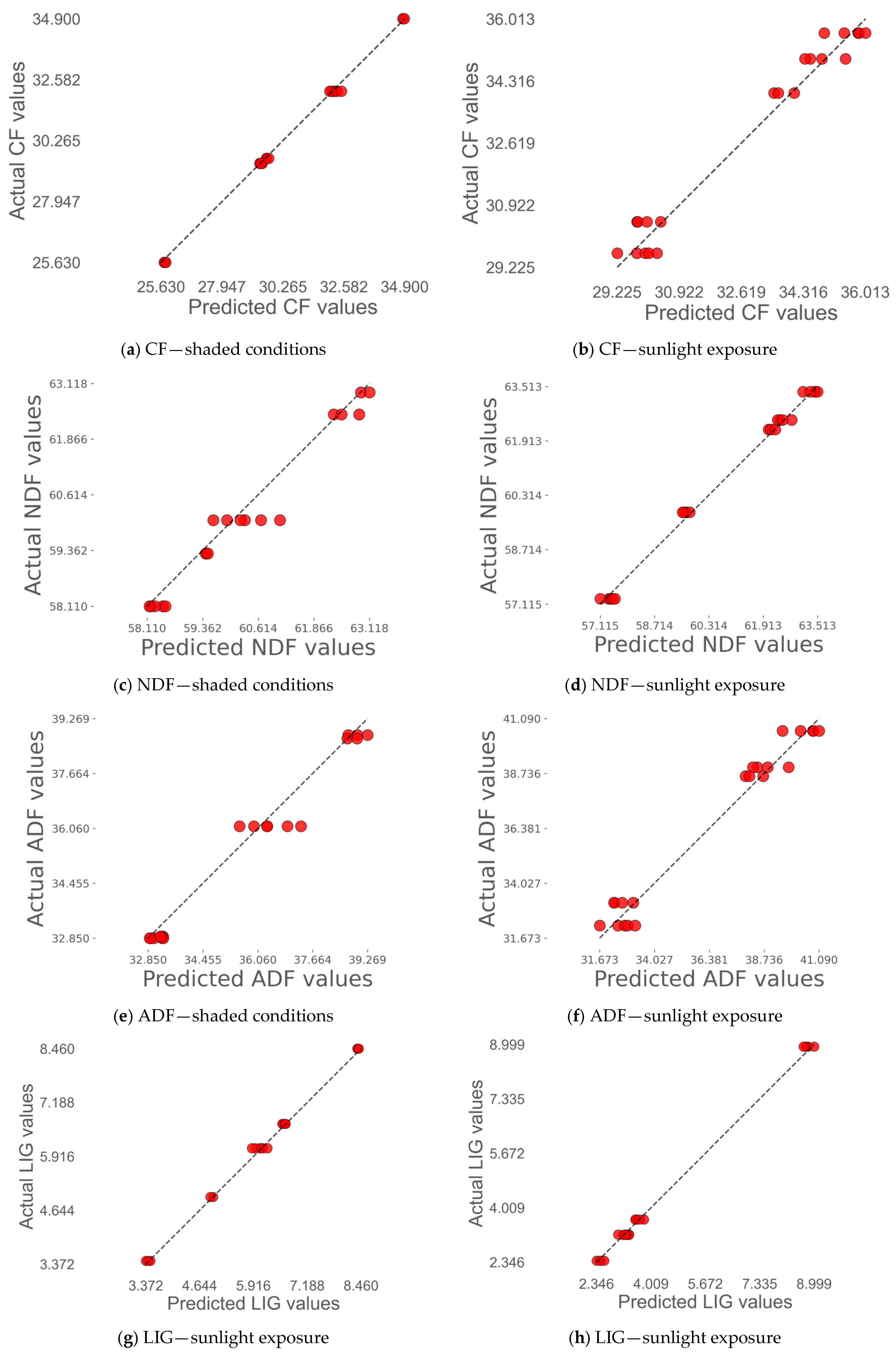
4.3.2. Prediction of Quality Traits

Similar to how biomass was predicted, the quality traits of the forage were processed using the six ML models with a cross-validation criterion. The graphical results are summarized in Figure 8.

Similar to the selection of biomass predictors, a permutation test identified the most relevant variables for the model.

Table 10. Quality traits predicted by ML models: In-field predictors and optical predictors indicated as x. R-H: Ridge hyperparameter, DT-H: Decision Tree hyperparameters, HT: Height of tussock, NP: Number of pixels, GR: Greenness, GLT: Green leaves per tussock.

Predicted Forage Variables	Condition				In-Field Predictors					Optical Predictors
		R-H	DT-H		D a t e	HT	GLT	GR	NP	C L R E	V A R I	N L I	E V I 2	R D V I	S A V I	S A R V I	S A R V I 2	R	N D V I	A R V I	A R V I 2
		α	MD	MF
CF	Sunlight	0.2	7	30		x	x		x				x				x	x	x		x
	Shaded	1.0	4	30	x					x	x	x	x			x	x			x
ADF	Sunlight	0.8	5	30	x	x					x	x	x		x	x	x
	Shaded	1.0	4	30	x		x		x		x	x	x		x		x
NDF	Sunlight	1.0	7	30	x	x					x	x	x		x	x	x
	Shaded	0.2	9	20	x	x					x	x	x	x	x		x
LIG	Sunlight	0.2	5	20	x	x					x	x	x		x	x	x
	Shaded	0.2	5	30						x	x	x	x			x	x			x
CP	Sunlight	0.2	4	30	x		x				x	x	x		x	x	x
	Shaded	0.2	9	30	x	x					x	x	x		x	x	x
EE	Sunlight	0.2			x	x	x				x	x	x		x		x
	Shaded	0.2	4	30	x	x	x				x	x	x		x		x
ASH	Sunlight	0.2	9	30	x	x					x	x	x		x	x	x
	Shaded	0.2	9	30	x			x		x	x	x	x			x				x

summarizes the results of quality traits predicted by various machine learning (ML) models and optical predictors. It provides insights into the most relevant predictors identified for each trait, offering a comprehensive overview of the relationships between optical parameters and the performance of the models.

5. Discussion

Forage biomass and quality prediction have seen tremendous development in recent years. The availability of satellite information and drone-based image capture has promoted a significant change in decision making in agriculture [33,34]. In fact, several commercial and research efforts using remote sensing tools have deployed new strategies to enhance accurate prediction. For instance, despite biomass forage prediction being lower than estimated by direct in-field measurements, image analysis provides over 60–80% accurate predictions when limited resources and data are available [33]. Reported machine learning (ML) models achieved an R² of 0.71 for biomass estimation, indicating a strong correlation between predicted and observed values [35]. However, the accuracy was lower for forage quality traits, reflecting the greater complexity and variability associated with these parameters. Additionally, the median normalized root mean square error (nRMSE) was approximately 13% for forage quality prediction, suggesting a moderate level of predictive reliability [36]. These results highlight the potential of the approach while also indicating areas for improvement in the estimation of forage quality attributes. Our study demonstrates high predictive accuracy, achieving R² values ranging from 0.938 to 0.998 for biomass and forage quality estimation. These results were obtained using 200 samples for model training with machine learning algorithms. The implementation of this approach requires a few informatic requirements, including sufficient computational capacity for data processing, access to sensor-based data collection, and software capable of handling machine learning models. These elements ensure the efficient application of AI-driven predictions in silvopastoral systems.

However, in some environmental scenarios with large variations, such as the tropics, remote sensing has shown low performance, mainly due to pasture diversity, especially when considering the presence of both grass and legumes in the plot [37,38]. Spectral characteristics and structural variability make it harder for machine learning models to generalize effectively; therefore, identifying either strategy or tools to increase predictability is fundamental [39]. Several strategies can be implemented to enhance model performance, including (1) Advanced Remote Sensing—Multispectral and hyperspectral imaging and sensors enhance species differentiation and biomass estimation accuracy; (2) Feature Engineering—Integrating soil properties, historical weather, and plant phenology improves model robustness; (3) Ensemble Learning—Combining models (e.g., random forests, gradient boosting) captures complex relationships more effectively; (4) Domain Adaptation—Transfer learning techniques enhance model adaptability across environmental conditions; (5) Automated Data Labeling—Expert-labeled and semi-supervised learning improve species differentiation; and (6) Mobile and Edge Computing—Real-time processing on mobile devices supports localized predictions, reducing reliance on centralized models. However, many of these are still in the research phase and in the process of building their scientific foundation. Therefore, at a practical level, the use of remote sensors and traditional vegetation indices remains common despite their low predictive capacity. For example, vegetation indices derived from remote sensors (drones or satellites) can be used for biomass estimation, with the Normalized Difference Vegetation Index (NDVI) being the most popular. However, under the experimental conditions, the NVDI was outperformed by other indexes for the prediction of biomass and quality traits of the forage. The combination of legumes and grasses can lead to low performance of some vegetation indexes like the NDVI, and information derived from wide spectra (hyperspectral sensors) or seasonal measurements [39,40] could enhance biomass prediction [41]. The low prediction capacity could be attributed to the spectral bands of commercial equipment detectors and satellite optical detectors, which are typically around 20–40 nm (see, for example, the bands of the optical sensors of the DJI drone and the Sentinel satellite) compared to the equipment used in this study, which has spectral bands of approximately 1 nm. Optical detection in broad bands (tens of nanometers) no longer corresponds to a single wavelength but rather to a spectral average within the band, incorporating neighboring wavelengths. This can introduce noise and generate inaccurate values in the measurement of intensity and reflectance, especially in the NIR bands whose slope is highly sensitive to changes in moisture and plant morphology, as in the case of deciduous trees [25].

In this work, the strategies mentioned above were used to enhance model performance. As a result, our findings demonstrate that it is possible to predict biomass and quality traits using linear regression ML models, such as LASSO, Ridge, and ElasticNet, with both optical and visual variables of tussocks as predictors. Furthermore, data engineering of VIS-NIR optical spectra to encode biomass and quality traits, combined with image segmentation and covariance strategies to achieve high performance by introducing categorical variables, were key highlights of this innovative approach. Additionally, the selection of eight features allowed for model simplification without compromising robustness. One of the most relevant predictors was tussock height, as observed for all parameters (biomass and quality traits) under sunlight exposure. In contrast, under shaded conditions, the predictors appeared to be more optical and categorical variables, reinforcing our hypothesis that this proposal of an optical system is more suitable for silvopastoral systems with trees present.

The results of this research directly address the practical management challenges in field-based livestock systems. The integration of VIS-NIR optical spectrometers, RGB cameras, and machine learning models into in-field forage monitoring will provide farmers with real-time data on pasture biomass and quality. This capability enables producers to make timely decisions on grazing management, improving feeding efficiency and pasture utilization. For example, having immediate access to accurate forage data will allow farmers to optimize grazing rotations, avoid overgrazing, and ensure that cattle receive the necessary nutrition. Additionally, this technology reduces the need for intensive laboratory analysis and costly work, directly benefiting producers by providing practical and cost-effective solutions that enhance productivity and sustainability.

Regarding practical implementation, machine learning (ML) models serve as the foundation for APIs, which play a crucial role in simplifying model development, enabling secure and efficient deployment, facilitating continuous learning, enhancing service recommendations, and improving the accessibility and usability of ML models across various domains, including web platforms and applications on operating systems such as Android and iOS [42].

The results represent a progression beyond recent proposals for using handheld VIS-NIR spectrometry in forage characterization [5,36]. Through the incorporation of other handheld equipment, such as smartphone cameras, we envision that ground-based technologies, assisted with data processing tools, offer a promising solution for predicting biomass and quality traits in forage. This study focuses on constructing prediction models using machine learning techniques, which are one of the main strategies for developing artificial intelligence systems. Supervised prediction techniques have been chosen as they tend to be more precise and reliable because of learning from labeled data.

Unlike spectrometers, multispectral cameras can generate 2D information (images) for imagery visualization. However, the specificity of this information in terms of vegetation identification is limited to using a few spectral bands. The availability of a greater amount of spectral data from a high-resolution spectral signature can uniquely characterize vegetation, a significant advantage in using high-resolution spectrometry on the ground. Optical information establishes a relationship with forage quality variables. The image provides valuable information on greenness and the number of pixels, which can improve prediction for other types of forage and even serve as a plant classifier. The study conducted here has focused on a single type of forage, and its validity can be extended to future research that confirms these findings in different species, distinguishing them by their shape, growth pattern, and greenness.

Silvopastoral systems, characterized by the coexistence of trees and pasture, present unique challenges for remote sensing technologies. In these arrangements, traditional remote sensing methods struggle due to limitations in capturing the canopy and the variations in the physical environment caused by tree cover [23,43]. While remote sensing is useful in many contexts, it often fails to capture the heterogeneous nature of these systems, which are limited by sensor resolution, the distance at which data is recorded, and environmental changes, for example, clouds on satellite images.

Scaling handheld sensors and machine learning techniques to different environments presents challenges such as sensor variability, environmental influences on readings, and difficulties in generalizing data across different climates and vegetation. Standardizing data collection with these devices is essential to reduce inconsistencies, while computational limitations may hinder real-time processing. Ensuring interoperability between data sources, addressing high costs and accessibility issues, and providing user training with intuitive interfaces are crucial for widespread adoption and usability.

Our findings suggest that ground-based technologies, providing more localized and specific data spectrometry, can bridge this gap, offering a more accurate and targeted solution for assessing forage quality in these complex systems. In addition, VIS-NIR spectrometer technology offers many more wavelengths (around one thousand) with high spectral precision (less than 1 nm) compared to the technical characteristics of multispectral cameras used in remote sensing, which are limited to only tens of wavelengths with low precision in terms of its optical band (between 20 and 40 nm of band).

It is important to acknowledge some potential challenges, such as the integration of multiple data sources—optical, environmental, and meteorological—which requires robust data processing and model calibration to ensure accuracy. Future research should focus on refining the models, enhancing data collection methods, sensor limitations, data variability, and computational constraints, and testing the technology under diverse environmental conditions to validate its effectiveness across different systems. Additionally, enhancing user adoption through intuitive tools and training is essential. Opportunities lie in leveraging advanced machine learning techniques, expanding datasets, and incorporating multispectral imaging for more precise forage assessment. Cloud-based solutions and mobile applications can improve accessibility, while a stronger focus on sustainability and precision agriculture can optimize resource use and support smart farming.

Another aspect to be tackled would be to ensure the adaptation and validation of these models with the limited wavelengths and optical characteristics of multispectral cameras, highlighting the inherent advantages of remote sensing technology. It is essential that these systems achieve appropriate technical refinement from an engineering standpoint yet remain simple enough to be adopted by stakeholders who are not experts.

Practical Applications

• Forage Monitoring and Management:

The practical applications of this development cover various areas within agricultural management, precision farming, and livestock management.

First, it facilitates forage monitoring and management, allowing livestock farmers to assess forage biomass and quality without the need for destructive sampling. This improves decision making regarding pasture management and livestock feed supplementation, optimizing available resources and reducing operational costs.

This work is particularly useful in silvopastoral systems, where the coexistence of trees and pastures presents challenges for traditional remote sensing with satellites and UAVs. By improving forage characterization in these environments, producers can more accurately adjust grazing strategies and livestock stocking rates, ensuring efficient utilization of grazing areas.

• Integration with digital tools and technological adoption to promote usability and practical applications.

To enhance usability and practicality, integration with digital tools and mobile applications is a key challenge. This development can be implemented on artificial intelligence-based platforms accessible from mobile devices, facilitating field monitoring. Additionally, a challenge lies in ensuring compatibility with APIs and integrating spectral technology with image processing technology to enable its use in an integrated system, including its incorporation into other agricultural and livestock applications, promoting greater technological adoption in the sector.

• Sustainability and data-driven decision making

In terms of forage yield prediction, this development would help anticipate changes in forage availability under different environmental conditions. This allows producers to take preventive measures against adverse climatic events, optimizing grazing planning and ensuring the sustainability of the production system.

Sustainability and precision agriculture also benefit from this approach, as spectral data-based models allow for the optimization of agricultural input usage. By understanding forage quality, costs on inputs can be reduced while minimizing environmental impact, promoting more efficient and sustainable production.

Furthermore, this development supports research and development in agricultural systems by promoting a machine-learning-based methodology that enables detailed analysis of pasture growth and nutritional quality using visual and optical predictors. One challenge is the “self-adjustment” of prediction models through the incorporation of more data, facilitating the validation of predictive models for different forage species and agroclimatic conditions, fostering innovation in the sector.

• Scalability and Future Prospects

Finally, from a technological development perspective, its scalability and adaptation to new technologies make it a flexible and versatile solution. The possibility of integration with cloud-based systems allows real-time data processing and analysis. These features ensure its applicability in various productive environments, strengthening data-driven decision making in the agricultural sector.

6. Conclusions

This research highlights the selection of key visual and optical parameters essential for model development, ensuring adaptability to other forage types. From an engineering perspective, the study underscores the integration of smartphones as a crucial component in enhancing technology accessibility and usability for stakeholders. This would be achieved using integration platforms (API, cloud, interactive interfaces), thereby facilitating the development of intelligent systems that address the real needs of producers in the context of animal welfare management.

This study demonstrates the potential of handheld proximal sensors combined with advanced machine learning techniques for accurate and cost-effective in-field forage quality prediction in silvopastoral systems. By incorporating Mahalanobis distance-based image segmentation and spectral feature extraction, we enhanced the precision of biomass and forage quality assessments, particularly for Mombasa grass.

Despite its advantages, the study has certain limitations. The accuracy of the models depends on the specific sensors used, which may not perform equally well with other devices from other manufacturers; however, other devices can be adapted to achieve similar results. Environmental factors such as lighting, humidity, and shadows in silvopastoral systems can affect image quality and spectral measurements. This issue can be addressed by using strategically placed spectral white calibration, as proposed in [12]. Additionally, the model was trained with data specific to Mombasa grass in a particular region and requires further validation for other forage species and agroclimatic conditions. The computational requirements of techniques such as Mahalanobis distance segmentation and spectral feature extraction may also pose challenges in low-resource environments. Furthermore, successful field implementation depends on digital infrastructure and user adoption, highlighting the need for accessible technology and adequate training for producers.

Future research should focus on refining these approaches, improving model adaptability, and expanding their application to other forage species and diverse environmental conditions.

References

1. Beeri, O.; Phillips, R.; Hendrickson, J.; Frank, A.B.; Kronberg, S. Estimating Forage Quantity and Quality Using Aerial Hyperspectral Imagery for Northern Mixed-Grass Prairie. Remote Sens. Environ. 2007, 110, 216–225. [Google Scholar] [CrossRef]
2. Geipel, J.; Bakken, A.K.; Jørgensen, M.; Korsaeth, A. Forage Yield and Quality Estimation by Means of UAV and Hyperspectral Imaging. Precis. Agric. 2021, 22, 1437–1463. [Google Scholar] [CrossRef]
3. Edvan, R.; Bezerra, L.; Marques, C.; Carneiro, M.S.; Oliveira, R.; Ferreira, R. Methods for Estimating Forage Mass in Pastures in a Tropical Climate. Rev. Ciências Agrárias 2016, 39, 36–45. [Google Scholar] [CrossRef]
4. Jank, L.; Valle, C.B.; Resende, R. Brazilian Society of Plant Breeding. Printed in Brazil Breeding Tropical Forages; Brazilian Society of Plant Breeding: Londrina, Brazil, 2011; Volume 1. [Google Scholar]
5. Mendes de Oliveira, D.; Pasquini, C.; Rita de Araújo Nogueira, A.; Dias Rabelo, M.; Lúcia Ferreira Simeone, M.; Batista de Souza, G. Comparative Analysis of Compact and Benchtop Near-Infrared Spectrometers for Forage Nutritional Trait Measurements. Microchem. J. 2024, 196, 109682. [Google Scholar] [CrossRef]
6. Gao, J.; Liang, T.; Liu, J.; Zhang, D.; Wu, C.; Feng, Q.; Xie, H. Hyperspectral remote sensing of forage stoichiometric ratios in the senescent stage of alpine grasslands. Field Crops Res. 2024, 313, 108027. [Google Scholar] [CrossRef]
7. Hennessy, A.; Clarke, K.; Lewis, M. Hyperspectral Classification of Plants: A Review of Waveband Selection Generalisability. Remote Sens. 2020, 12, 113. [Google Scholar] [CrossRef]
8. Tedesco, D.; Nieto, L.; Hernández, C.; Rybecky, J.; Min, D.; Sharda, A.; Hamilton, K.; Ciampitti, I. Remote Sensing on Alfalfa as an Approach to Optimize Production Outcomes: A Review of Evidence and Directions for Future Assessments. Remote Sens. 2022, 14, 4940. [Google Scholar] [CrossRef]
9. Condran, S.; Bewong, M.; Islam, M.Z.; Maphosa, L.; Zheng, L. Machine Learning in Precision Agriculture: A Survey on Trends, Applications and Evaluations over Two Decades. IEEE Access 2022, 10, 73786–73803. [Google Scholar] [CrossRef]
10. Liakos, K.; Busato, P.; Moshou, D.; Pearson, S.; Bochtis, D. Machine Learning in Agriculture: A Review. Sensors 2018, 18, 2674. [Google Scholar] [CrossRef]
11. Zhou, Z.; Morel, J.; Parsons, D.; Kucheryavskiy, S.V.; Gustavsson, A.M. Estimation of Yield and Quality of Legume and Grass Mixtures Using Partial Least Squares and Support Vector Machine Analysis of Spectral Data. Comput. Electron. Agric. 2019, 162, 246–253. [Google Scholar] [CrossRef]
12. Cevoli, C.; Di Cecilia, L.; Ferrari, L.; Fabbri, A.; Molari, G. Evaluation of Cut Alfalfa Moisture Content and Operative Conditions by Hyperspectral Imaging Combined with Chemometric Tools: In-Field Application. Biosyst. Eng. 2022, 222, 132–141. [Google Scholar] [CrossRef]
13. Zhang, Y.; Zhao, D.; Liu, H.; Huang, X.; Deng, J.; Jia, R.; He, X.; Tahir, M.N.; Lan, Y. Research Hotspots and Frontiers in Agricultural Multispectral Technology: Bibliometrics and Scientometrics Analysis of the Web of Science. Front. Plant Sci. 2022, 13, 955340. [Google Scholar] [CrossRef]
14. Liu, H.; Bruning, B.; Garnett, T.; Berger, B. Hyperspectral Imaging and 3D Technologies for Plant Phenotyping: From Satellite to Close-Range Sensing. Comput. Electron. Agric. 2020, 175, 105621. [Google Scholar]
15. Gates, D.M.; Keegan, H.J.; Schleter, J.C.; Weidner, V.R. Spectral Properties of Plants. Appl. Opt. 1965, 4, 11–20. [Google Scholar] [CrossRef]
16. Dymond, J.R.; Shepherd, J.D.; Qi, J. A Simple Physical Model of Vegetation Reflectance for Standardising Optical Satellite Imagery. Remote Sens. Environ. 2001, 75, 350–359. [Google Scholar] [CrossRef]
17. Edward, B. Physical and Physiological Basis for the Reflectance of Visible and Near-Infrared Radiation from Vegetation. Remote Sens. Environ. 1970, 1, 155–159. [Google Scholar]
18. Rao, N.R. Development of a Crop-Specific Spectral Library and Discrimination of Various Agricultural Crop Varieties Using Hyperspectral Imagery. Int. J. Remote Sens. 2008, 29, 131–144. [Google Scholar] [CrossRef]
19. Singh, V.; Sharma, N.; Singh, S. A Review of Imaging Techniques for Plant Disease Detection. Artif. Intell. Agric. 2020, 4, 229–242. [Google Scholar]
20. Zamft, B.M.; Conrado, R.J. Engineering Plants to Reflect Light: Strategies for Engineering Water-Efficient Plants to Adapt to a Changing Climate. Plant Biotechnol. J. 2015, 13, 867–874. [Google Scholar] [CrossRef]
21. Mangold, K.; Shaw, J.A.; Vollmer, M. The Physics of Near-Infrared Photography. Eur. J. Phys. 2013, 34, S51. [Google Scholar] [CrossRef]
22. Kothari, S.; Schweiger, A.K. Plant Spectra as Integrative Measures of Plant Phenotypes. J. Ecol. 2022, 110, 2536–2554. [Google Scholar]
23. Tucker, C. Spectral Estimation of Grass Canopy Variables. Remote Sens. Environ. 1977, 6, 11–26. [Google Scholar] [CrossRef]
24. Ahamed, T.; Tian, L.; Zhang, Y.; Ting, K.C. A Review of Remote Sensing Methods for Biomass Feedstock Production. Biomass Bioenergy 2011, 35, 2455–2469. [Google Scholar]
25. Araus, J.L.; Kefauver, S.C.; Vergara-Díaz, O.; Gracia-Romero, A.; Rezzouk, F.Z.; Segarra, J.; Buchaillot, M.L.; Chang-Espino, M.; Vatter, T.; Sanchez-Bragado, R.; et al. Crop Phenotyping in a Context of Global Change: What to Measure and How to Do It. J. Integr. Plant Biol. 2022, 64, 592–618. [Google Scholar]
26. Cook, C.W. Symposium on Nutrition of Forages and Pastures: Collecting Forage Samples Representative of Ingested Material of Grazing Animals for Nutritional Studies. J. Anim. Sci. 1964, 23, 265–270. [Google Scholar] [CrossRef]
27. Weiss, W.P.; Hall, M.B. Laboratory Methods for Evaluating Forage Quality. In Forages; Wiley Online Library: Hoboken, NJ, USA, 2020; pp. 659–672. ISBN 9781119436669. [Google Scholar]
28. Hernández Molina, D.D.; Gulfo Galaraga, J.M.; López López, A.M.; Serpa Imbett, C.M. Methods for estimating agricultural cropland yield based on the comparison of NDVI images analyzed by means of Image segmentation algorithms: A tool for spatial planning decisions. Ingeniare. Rev. Chil. Ing. 2023, 31, 224–235. [Google Scholar]
29. Wang, Z.; Wang, E.; Zhu, Y. Image Segmentation Evaluation: A Survey of Methods. Artif. Intell. Rev. 2020, 53, 5637–5674. [Google Scholar] [CrossRef]
30. Zhang, Y.; Huang, D.; Ji, M.; Xie, F. Image Segmentation Using PSO and PCM with Mahalanobis Distance. Expert Syst. Appl. 2011, 38, 9036–9040. [Google Scholar] [CrossRef]
31. Zhou, Z.H. Machine Learning; Springer Nature: Berlin/Heidelberg, Germany, 2021; ISBN 9789811519673. [Google Scholar]
32. Raheem, M.A.; Udoh, N.S.; Gbolahan, A.T. Choosing Appropriate Regression Model in the Presence of Multicolinearity. Open J. Stat. 2019, 09, 159–168. [Google Scholar] [CrossRef]
33. Théau, J.; Lauzier-Hudon, É.; Aubé, L.; Devillers, N. Estimation of Forage Biomass and Vegetation Cover in Grasslands Using UAV Imagery. PLoS ONE 2021, 16, e0245784. [Google Scholar] [CrossRef]
34. Nguyen, P.T.; Shi, F.; Wang, J.; Badenhorst, P.E.; Spangenberg, G.C.; Smith, K.F.; Daetwyler, H.D. Within and Combined Season Prediction Models for Perennial Ryegrass Biomass Yield Using Ground- and Air-Based Sensor Data. Front. Plant Sci. 2022, 13, 950720. [Google Scholar] [CrossRef] [PubMed]
35. Gámez, A.L.; Vatter, T.; Santesteban, L.G.; Araus, J.L.; Aranjuelo, I. Onfield Estimation of Quality Parameters in Alfalfa through Hyperspectral Spectrometer Data. Comput. Electron. Agric. 2024, 216, 108463. [Google Scholar] [CrossRef]
36. Wijesingha, J.; Astor, T.; Schulze-Brüninghoff, D.; Wengert, M.; Wachendorf, M. Predicting Forage Quality of Grasslands Using UAV-Borne Imaging Spectroscopy. Remote Sens. 2020, 12, 126. [Google Scholar] [CrossRef]
37. Kawamura, K.; Tanaka, T.; Yasuda, T.; Okoshi, S.; Hanada, M.; Doi, K.; Saigusa, T.; Yagi, T.; Sudo, K.; Okumura, K.; et al. Legume Content Estimation from UAV Image in Grass-Legume Meadows: Comparison Methods Based on the UAV Coverage vs. Field Biomass. Sci. Rep. 2024, 14, 31705. [Google Scholar] [CrossRef]
38. Villoslada Peciña, M.; Bergamo, T.F.; Ward, R.D.; Joyce, C.B.; Sepp, K. A Novel UAV-Based Approach for Biomass Prediction and Grassland Structure Assessment in Coastal Meadows. Ecol. Indic. 2021, 122, 107227. [Google Scholar] [CrossRef]
39. McCann, J.A.; Keith, D.A.; Kingsford, R.T. Measuring Plant Biomass Remotely Using Drones in Arid Landscapes. Ecol. Evol. 2022, 12, e8891. [Google Scholar] [CrossRef]
40. Bazzo, C.O.G.; Kamali, B.; Hütt, C.; Bareth, G.; Gaiser, T. A Review of Estimation Methods for Aboveground Biomass in Grasslands Using UAV. Remote Sens. 2023, 15, 639. [Google Scholar] [CrossRef]
41. Zhu, X.; Liu, D. Improving Forest Aboveground Biomass Estimation Using Seasonal Landsat NDVI Time-Series. ISPRS J. Photogramm. Remote Sens. 2015, 102, 222–231. [Google Scholar] [CrossRef]
42. Leenings, R.; Winter, N.R.; Plagwitz, L.; Holstein, V.; Ernsting, J.; Sarink, K.; Fisch, L.; Steenweg, J.; Kleine-Vennekate, L.; Gebker, J.; et al. PHOTONAI—A Python API for Rapid Machine Learning Model Development. PLoS ONE 2021, 16, e0254062. [Google Scholar] [CrossRef]
43. Cherney, J.H.; Digman, M.F.; Cherney, D.J. Handheld NIRS for Forage Evaluation. Comput. Electron. Agric. 2021, 190, 106469. [Google Scholar] [CrossRef]
Figure 1. Study setting: a paddock (in the rectangle) selected within the SBPM with Mombasa grass and featuring scattered trees (in circles).
Agriengineering 07 00111 g001
Figure 2. Spatial distribution of sampling geolocation in the paddock for understanding the heterogeneity of growth conditions within the silvopastoral system. The colored symbols are: blue for day 7, orange for day 14, green for day 21, red for day 28, and magenta for day 35 (a) All samples, (b) geolocation in the shaded condition, (c) geolocation under sunlight exposure.
Agriengineering 07 00111 g002
Figure 3. Illustration of the methodology for capturing spectral signatures using an SR-4VN500-5 Ocean Insight optical spectrometer with optical fiber and Ghersum tubes. (a) Set up for the four spectral captures. (b) Zenithal perspective to obtain the four (4) spectral signatures at different azimuthal positions around the tussock. (c) Measurements of each spectrum at a zenithal angle of 45° to capture canopy radiation.
Agriengineering 07 00111 g003
Figure 4. Unprocessed spectra taken from tussock 18 over five sessions. λ is the light wavelength in nm (nanometers), and %R is the percentage of reflectance. The red line indicates the mean of the four spectra on (a) day 7, (b) day 14, (c) day 21, (d) day 28, and (e) day 35 of regrowth.
Agriengineering 07 00111 g004aAgriengineering 07 00111 g004b
Figure 5. Steps to implement the Mahalanobis distance algorithm to segment images: (a) Unprocessed images. (b) Selected green pixel values (100 classes) were used to obtain the mean and inverse covariance matrix for executing the Mahalanobis algorithm. (c) Processed and segmented images.
Agriengineering 07 00111 g005
Figure 6. Radar diagram showing higher NIR covariance (CovNIR) compared to R (CovR), G (CovG), B (CovB), and RE (CovRE) covariance values. (a) CovNIR is higher compared to others. (b) CovNIR is higher compared to others but less than (a). (c) CovNIR is higher compared to (a).
Agriengineering 07 00111 g006aAgriengineering 07 00111 g006b
Figure 7. Predicted dry matter (g) values based on ML models. (a) ElasticNet ML model under shaded condition. (b) LASSO under sunlight exposure.
Agriengineering 07 00111 g007
Figure 8. Predicted quality traits vs. training set based on the Ridge ML model. (a,c,e,g,i,k,m) are predicted quality traits under shaded conditions; (b,d,f,h,j,l,n) are predicted quality traits under sunlight exposure.
Agriengineering 07 00111 g008aAgriengineering 07 00111 g008b