1. Introduction
Global food security requires a 50% increase in crop yields by 2050, yet achieving this goal is increasingly difficult due to shrinking arable land, resource inefficiencies, and climate change [
1]. Productivity in agriculture is also endangered by extreme weather events and soil erosion, lowering the overall resilience of crops [
2]. Weed competition is among the key limitations to improved crop yields, as weeds greatly compete with crops for nutrients, water, and light, leading to tremendous yield losses [
3]. Pesticides and manual weeding have been conventionally employed by farmers, but they are beset with high costs, inefficiencies, and environmental concerns [
4]. Accordingly, AI-based precision agriculture technologies have been a promising solution, facilitating automated and highly precise weed detection [
5]. Among these innovations, Unmanned Aerial Vehicles (UAVs) have been a vital enabler for precision agriculture, providing high-resolution imagery and real-time flexibility in comparison to conventional remote sensing methods [
6]. The integration of deep learning (DL) techniques with UAV-based imagery has also greatly enhanced automatic weed detection, particularly through the use of semantic segmentation techniques [
7]. It has also enhanced field boundary mapping, crop health assessment, and land use classification greatly [
8].
Still, irrespective of these technological advances, a few major challenges still persist. Most DL-based weed segmentation models fail to efficiently identify both local and global contextual features, resulting in segmentation failure, particularly in complicated weed/crop overlap situations [
9]. Also, these models tend to have low boundary accuracy, which complicates distinguishing between fine differences between crops and weeds in UAV images [
10]. But, yet another important limitation is the huge computational cost associated with cutting-edge deep learning models, precluding their deployment in practical implementations on resource-limited UAVs [
11]. Although DL algorithms have been found to provide improved accuracy, they do not generalize across diverse situations and struggle with inconsistencies wrought by dissimilar illumination conditions, diverse weed biotypes, and diverse field settings [
12].
To tackle these challenges, we propose MSEA-Net, a novel segmentation framework that enhances contextual feature representation, boundary delineation, and computational efficiency. The key contributions of this study are summarized as follows:
- 1.
To enhance feature representation and efficiency, we design the Multi-Scale Attention Fusion (MSAF) module, which fuses multi-scale features while integrating spatial-channel recalibration to refine the importance of different feature representations. Additionally, MSAF employs a compact hierarchical design that eliminates redundant convolutions, reducing computational complexity while preserving rich semantic information.
- 2.
To improve boundary delineation, we propose the Edge-Enhanced Bottleneck Attention (EEBA) module, which incorporates edge-aware processing to refine object boundaries. By leveraging low-level edge features, this module improves segmentation precision, particularly in complex weed/crop overlap regions where texture similarity often leads to misclassification.
- 3.
To ensure computational efficiency, we design a lightweight architecture that minimizes the number of parameters and computational overhead, making the model deployable on resource-constrained UAVs for real-time weed segmentation.
- 4.
The proposed model is highly robust to environmental variability and generalizes well across diverse agricultural conditions, including variable lighting, complex backgrounds, and overlapping weed/crop regions.
Through comprehensive evaluation, we demonstrate that MSEA-Net outperforms existing state-of-the-art methods in precision, recall, F1-score, and mean IoU, validating its effectiveness across different agricultural conditions. The model achieves high segmentation accuracy while maintaining a compact architecture, making it suitable for real-time deployment on UAVs and other edge devices. By addressing key limitations in current UAV-based weed segmentation approaches, such as poor generalization, boundary misclassification, and high computational demands, this work contributes to advancing automated weed detection systems. Ultimately, MSEA-Net supports the development of more efficient, scalable, and sustainable agricultural practices, reducing the need for manual intervention and excessive herbicide use and enabling data-driven weed management at scale.
2. Literature Review
Recent research has carried out an intensive and comprehensive analysis of a number of approaches that leverage artificial intelligence for weed detection. This analysis highlights the importance of such approaches in the advancement of precision agriculture, alongside their contribution towards encouraging sustainable practices in weed management [
13,
14]. CNN-based models have also seen extensive application in the area of weed detection. To this end, the problem is addressed by framing the issue as a supervised classification problem, which allows for enhanced detection of unwanted plants [
15,
16].
Deep learning models such as AlexNet, GoogLeNet, InceptionV3, and Xception were attempted for weed identification with a maximum accuracy of 97.7% for RGB image-based classification [
17]. Weed detection using YOLO resulted in real-time performance improvements over standard CNN models [
18]. For improving spatial accuracy, models including UNet, SegNet, and DeepLabV3+ were utilized. Comparative analysis on the dataset CoFly-WeedDB showed that UNet with EfficientNetB0 yielded the optimal segmentation accuracy compared to other architectures [
19]. Experiments using UNet and its variations for weed segmentation in ground-based RGB images reported an Intersection over Union (IoU) score of 56% when utilizing UNet++ [
20]. Custom CNN models have been utilized to classify weeds in soybean fields with 98% accuracy. Still, the use of image-level classification instead of pixel-wise segmentation restricted the accuracy of such models [
21]. MobileNetV2-based light-weight architectures were suggested for UAV weed identification in order to achieve computational efficiency at the expense of boundary accuracy [
22].
Likewise, AlexNet has also been employed in the classification of weeds in Chinese cabbage fields with 92.41% accuracy, 6% above the accuracy of traditional classifiers like Random Forest [
23]. These observations point to the delicate balance between model complexity and the possibility of real-time UAV-based weed detection. Integrating visible color indices with deep learning segmentation models has enhanced the classification of weeds, a perspective that heralds more accurate herbicide application [
24]. The exploration of CGAN-based weed segmentation has revealed that the C-U-Net model boosts the mean Intersection over Union (mIoU) by 10%. Nevertheless, challenges such as data imbalance, corrupted samples, and the requirement for a more powerful penalizer and discriminator persist [
25]. Beyond single-stage CNN architectures, researchers have also investigated multi-stage classification pipelines to enhance segmentation accuracy further. A three-step method integrating Hough Transform for detecting crop rows with CNN-based segmentation has been proposed for weed detection in bean and spinach fields. However, its high sensitivity to changes in the background reduced adaptability to diverse field conditions [
26]. FG-UNet has been suggested for segmenting weeds but performed poorly on dense and complex weed distributions, limiting its use in practical applications [
27]. A U-Net version specifically developed for UAV-based weed segmentation showed promise but was held back by its use of a limited dataset and a simple architecture to be adequately versatile to varied crop conditions and complicated segmentation tasks [
28]. A segmentation pipeline using ground-based data was also suggested, but its adaptability to accommodate UAV images and plant growth stages is restricted [
29]. In the same vein, SSU-Net was also made to be more efficient; nonetheless, its dependence on high-quality training data and the necessity for a robust adaptation algorithm are still tremendous challenges [
30].
Though there has been significant progress in UAV-based image segmentation, some issues remain. They include segmentation errors in complicated overlaps between weeds and crops, boundary imprecision, computational expensiveness, and poor generalization in varied environments. Our work addresses these limitations by developing more efficient algorithms, enhancing model generalization, and improving the accuracy of UAV-based image segmentation for practical agricultural applications.
3. Material and Methods
3.1. Overview of the MSEA-Net
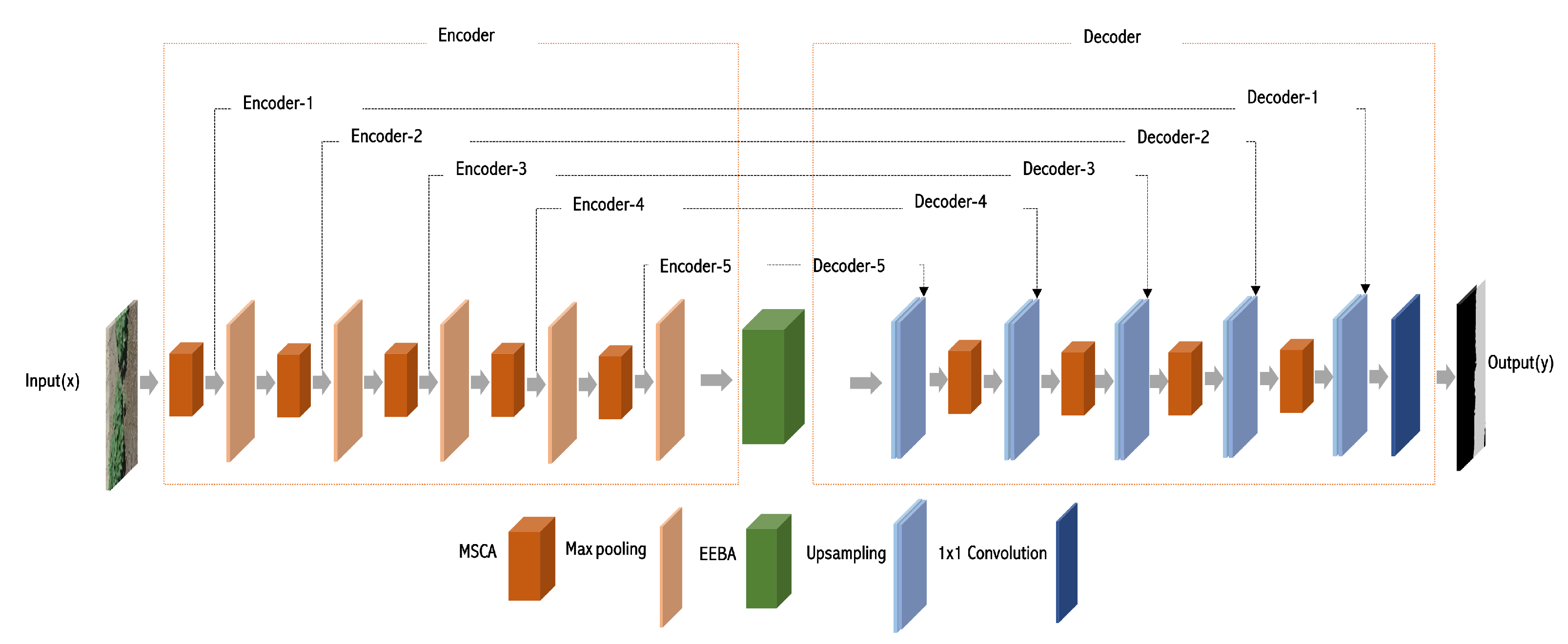
In this work, we propose MSEA-Net, a lightweight and efficient deep learning framework for accurate weed segmentation in precision agriculture. As illustrated in
Figure 1, MSEA-Net follows a hierarchical encoder–decoder architecture, where the encoder extracts multi-scale spatial features and the decoder reconstructs high-resolution segmentation maps. To achieve high segmentation accuracy with minimal computational overhead, MSEA-Net integrates two key modules: (1) the Multi-Scale Spatial-Channel Attention (MSCA) module (
Figure 2), which enhances multi-scale feature fusion and spatial-channel recalibration, and (2) the Edge-Enhanced Bottleneck Attention (EEBA) module (
Figure 3), which improves boundary delineation using edge information. The MSCA module employs hierarchical convolutions and spatial-channel recalibration to optimize multi-scale feature representation while reducing model complexity. Additionally, squeeze-and-excitation (SE) blocks are embedded to enhance channel-wise feature selection, where the EEBA module utilizes edge-aware processing to enhance object boundary refinement, effectively reducing weed/crop misclassification in complex agricultural settings. By incorporating these components into an optimized encoder–decoder framework, MSEA-Net achieves both high segmentation accuracy and computational efficiency. Its design facilitates robust feature extraction and precise boundary delineation while maintaining a lightweight architecture.
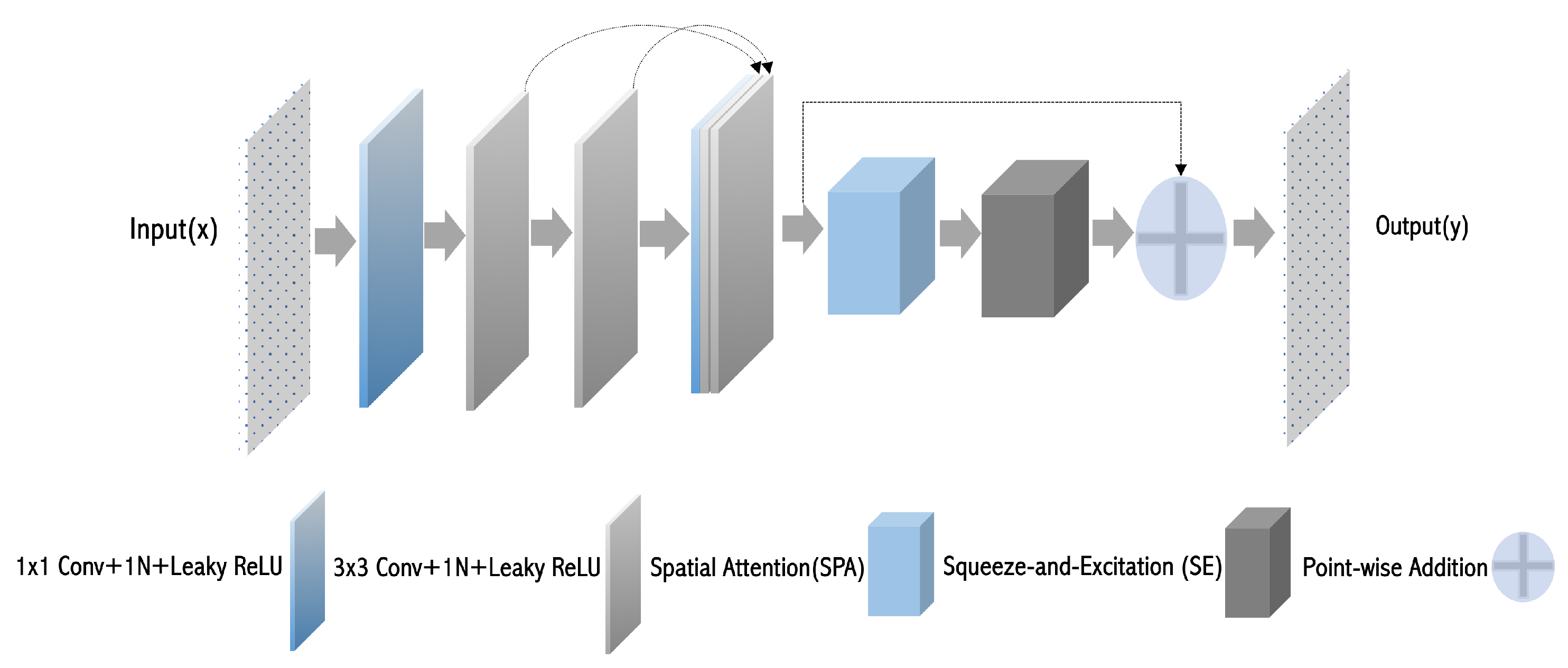
3.2. Multi-Scale Spatial-Channel Attention (MSCA) Module
A substantial body of research has shown that incorporating multi-scale features can significantly improve performance in image analysis tasks [
31,
32,
33]. However, many existing methods introduce increased parameter overhead and primarily focus on feature extraction while overlooking feature refinement and computational efficiency.
To address these limitations, the MSCA module is introduced, as illustrated in
Figure 2. Given an input feature map
, MSCA is specifically designed to extract and fuse multi-scale spatial features, allowing the model to effectively capture both local fine-grained details and global contextual information while optimizing computational efficiency. This is achieved through the integration of hierarchical convolutions, spatial attention mechanisms, and channel-wise recalibration, ensuring the extraction of meaningful multi-scale representations without excessive complexity.
3.2.1. Multi-Scale Feature Extraction and Fusion
To efficiently capture multi-scale information, the MSCA module employs a hierarchical convolutional structure. An initial
convolution reduces the feature map’s dimensionality, limiting computational overhead while preserving essential information. This is followed by two sequential
convolutions, which extract localized spatial patterns at different receptive fields. Instance normalization and LeakyReLU activation improve feature stability and non-linearity. This structure ensures that both local and global features are effectively extracted without excessive parameter growth. The extracted multi-scale features are then aggregated to form the fused representation:
where
represents the final fused feature representation, and
denote the feature maps extracted at different scales before concatenation. This operation ensures that fine and coarse spatial details are combined while preserving distinct multi-scale information.
3.2.2. Spatial Attention (SPA) Module
The SPA module, illustrated in
Figure 4, enhances spatially significant regions by selectively weighting feature map locations through a unified spatial refinement process. It employs depthwise convolutions, pointwise convolution, and residual connections to capture both localized and global spatial dependencies and enhance key regions for segmentation. The attention map is computed within this integrated refinement, and the refined spatial attention is fused with the original features via a residual connection to maintain stability and improve segmentation accuracy.
where
represents the refined feature map after applying spatial attention,
denotes the spatial attention map derived from the refinement process, and
is the concatenated multi-scale feature representation. This operation effectively reinforces spatial dependencies while maintaining stable and accurate feature representations.
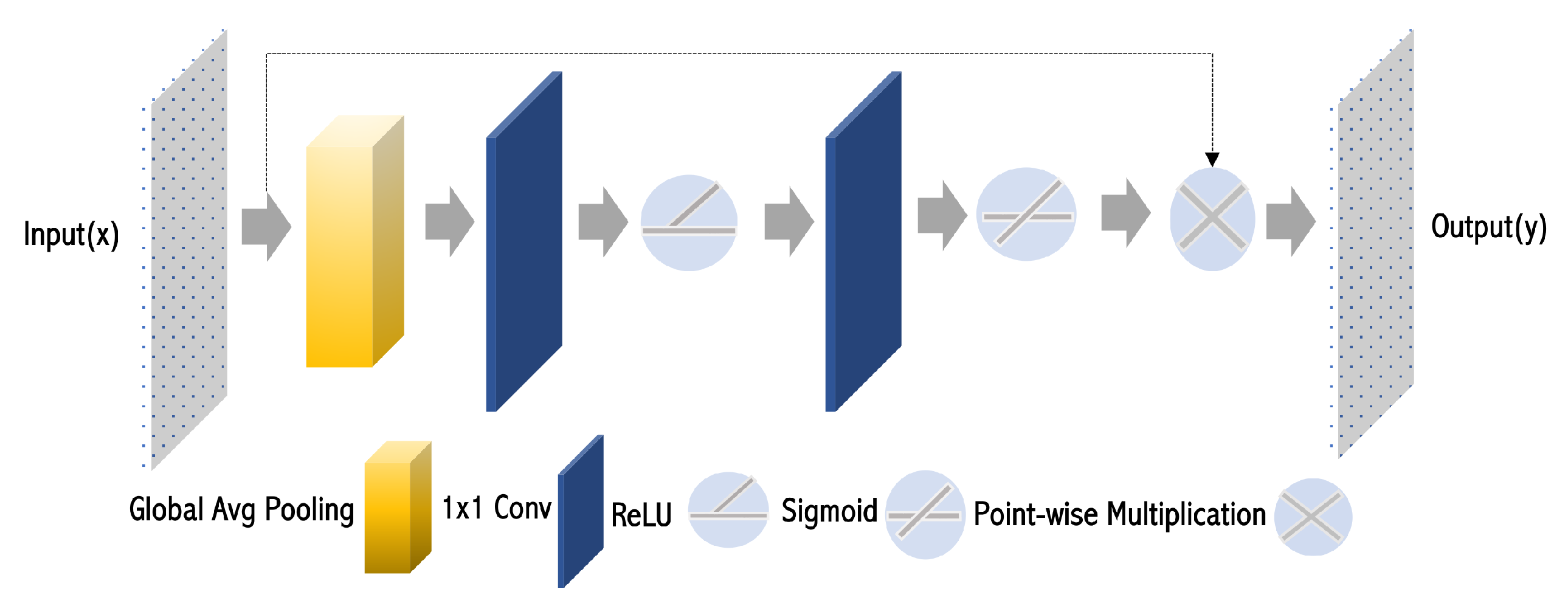
3.2.3. Channel-Wise Feature Enhancement
To further refine feature representations, a lightweight recalibration mechanism is applied using a squeeze-and-excitation (SE) block [
34], as illustrated in
Figure 5. SE enhances the most informative feature channels while suppressing redundant activations, allowing the model to focus on key feature responses. This recalibration is performed through global average pooling followed by channel-wise scaling, ensuring better feature discrimination.
To maintain the integrity of the multi-scale information, a residual skip connection is introduced, fusing the refined features with the original multi-scale representations:
This output integrates hierarchical feature extraction, spatial refinement, and recalibrated channel representations, making it robust for segmentation tasks.
3.3. Edge-Enhanced Bottleneck Attention (EEBA) Module
The EEBA module integrates edge-aware information with spatially refined features to enhance object boundary delineation while preserving global contextual information. This is particularly beneficial in segmentation tasks where precise boundary detection is essential, such as in precision agriculture. The overall structure of the EEBA module is illustrated in
Figure 3.
To enhance boundary precision, EEBA extracts edge-aware features from the encoder’s bottleneck feature map using the Sobel operator, which highlights regions of significant intensity change:
Here,
represents the encoder’s bottleneck feature map, and the Sobel operator extracts edge-aware features by detecting abrupt intensity variations, which typically correspond to object boundaries. This enhances segmentation accuracy, particularly in regions with fine structural details. These edge-aware features provide structural information that aids in distinguishing fine object boundaries, reducing segmentation errors in regions with high weed/crop overlap. To ensure that edge-aware features focus on significant spatial regions, they are refined using the SPA module, which enhances spatial dependencies, ensuring a stronger focus on key segmentation areas:
The SPA module refines the extracted edge features by selectively enhancing their spatial dependencies. This ensures that only the most relevant boundary information is retained while suppressing noise, leading to better feature representation for segmentation.
The refined edge-aware features are then fused with the encoder bottleneck output to integrate both fine-grained edge information and global feature representations:
By adding the refined edge-aware features to the original encoder output , the fused representation preserves both high-level contextual information and precise boundary details. This integration improves segmentation accuracy by maintaining structural integrity while incorporating semantic understanding. To improve efficiency while preserving structural details, the fused features undergo downsampling, reducing spatial resolution while retaining essential boundaries for decoding. The final EEBA output remains compact yet informative, ensuring precise segmentation with minimal computational overhead.
3.4. Loss Function
Effective weed segmentation requires loss functions that address class imbalance and ensure precise boundary delineation. Given that weeds often occupy a smaller proportion of the image than crops or background, appropriate loss selection is crucial to prevent model bias and misclassification.
3.4.1. Dice–Focal Loss
Binary weed segmentation involves distinguishing weeds from crops and background, often in imbalanced datasets. Dice–Focal Loss is adopted to enhance segmentation performance while mitigating class imbalance. Dice Loss optimizes the overlap between predicted and ground truth masks, ensuring robust segmentation even when weeds are irregularly shaped or sparsely distributed:
However, Dice Loss alone does not prioritize difficult-to-classify pixels. To address this, Focal Loss is incorporated, placing greater emphasis on misclassified regions:
The combined Dice–Focal Loss is formulated as:
where
balances the contributions of Dice and Focal Loss, and
adjusts the weighting for hard-to-classify pixels. This combination improves segmentation of small, dispersed weeds while addressing class imbalance.
3.4.2. Cross-Entropy Loss
Multi-class weed segmentation requires differentiation between multiple vegetation types. Cross-Entropy Loss is employed to ensure that underrepresented classes are adequately learned while maintaining overall classification accuracy:
where
C is the number of classes,
represents the ground truth probability for pixel
i in class
c, and
is the predicted probability for the same class. Unlike Dice–Focal Loss, which is designed for binary tasks, Cross-Entropy Loss effectively handles multiple class probabilities, ensuring that all vegetation types are properly segmented. Its selection ensures accurate classification in complex weed segmentation tasks with highly imbalanced class distributions.
4. Experiments
4.1. Dataset
4.1.1. CoFly-WeedDB
CoFly-WeedDB consists of 201 high-resolution RGB images captured over a cotton field in Greece using a DJI Phantom Pro 4 UAV. The images were taken from an altitude of 5 m, ensuring sufficient detail for precise segmentation. Each image includes pixel-level annotations categorizing the scene into three weed types—Johnson grass (Sorghum halepense), field bindweed (Convolvulus arvensis), and purslane (Portulaca oleracea)—along with the background. The dataset comprises images with a resolution of 1280 × 720 pixels; however, a significant class imbalance is evident. Pixel counts for Johnson grass, field bindweed, and background are approximately , , and , respectively, while purslane pixels total only . This imbalance presents a considerable challenge for segmentation tasks. We focused on distinguishing weeds from the background to improve model performance.
4.1.2. Motion-Blurred UAV Images of Sorghum Fields
For the second dataset, we utilized a publicly available UAV-captured dataset from an experimental sorghum field in Southern Germany [
36]. A consumer-grade drone—DJI Mavic 2 Pro equipped with a 20 MP Hasselblad camera (L1D-20c)—was employed for data collection, capturing images at a resolution of 5472 × 3648 pixels, with a ground sampling distance (GSD) of 1 mm, ensuring precision in distinguishing sorghum and weeds at early growth stages. Further technical specifications can be found in the publicly available source:
https://www.sciencedirect.com/science/article/pii/S0168169922006962?via%3Dihub#s0010, accessed on 10 October 2024. The dataset includes pixel-level annotations with three classes, i.e., sorghum, weeds, and soil. Expert supervision was employed to ensure high-quality ground truth. To facilitate model training and evaluation, 6300 image patches of 256 × 256 pixels were extracted from 19 images.
4.2. Implementation Details
Before being fed into the network, all images were preprocessed into 256 × 256 patches. To enhance generalization, various data augmentation techniques were applied, including horizontal and vertical flipping, random rotations, and grid distortion. The dataset was split into training (80%), validation (10%), and test (10%) sets. All hyperparameters were tuned using the validation set. To prevent overfitting, early stopping was employed, with training halted if the validation loss failed to improve over 20 consecutive epochs. All experiments were implemented in Python (all experiments were carried out using Python version 3.8.9) using the PyTorch (the implementation was conducted using PyTorch version 2.4.0) framework and conducted on an NVIDIA GeForce RTX 4090 (the experiments were performed on an NVIDIA GeForce RTX 4090 D GPU, manufactured by NVIDIA Corporation and procured from
https://global.jd.com/ (Beijing, China)). The hyperparameter settings used in the experiments are detailed in
Table 2.
4.3. Benchmark Method
To validate the effectiveness of the proposed model, we reproduce and compare it with several segmentation architectures and backbone CNNs used in [
19]. The segmentation models include SegNet, UNet, and DeepLabV3+, while the backbone CNNs are VGG16, ResNet50, DenseNet121, EfficientNetB0, and MobileNetV2. All comparisons are conducted using the same hyperparameters and identical preprocessing, training, and validation setups to ensure a fair and consistent benchmarking process.
4.4. Evaluation Metrics
The performance of the proposed model and benchmark methods is evaluated using the following metrics, as summarized in the comparison table:
Mean IoU (Intersection over Union): Represents the average overlap between predicted segmentation and ground truth across all classes, providing a standard measure of segmentation accuracy.
Precision: Defined as the ratio of correctly predicted positive pixels to the total predicted positive pixels, it evaluates the model’s ability to avoid false positives.
Recall: Calculated as the ratio of correctly predicted positive pixels to the total actual positive pixels, this metric assesses the model’s sensitivity.
F1-Score: The harmonic mean of precision and recall, balancing these two complementary metrics to capture overall prediction performance.
IoU (Background and Weed): Class-specific IoU scores computed separately for the background and weed classes to highlight per-class segmentation quality.
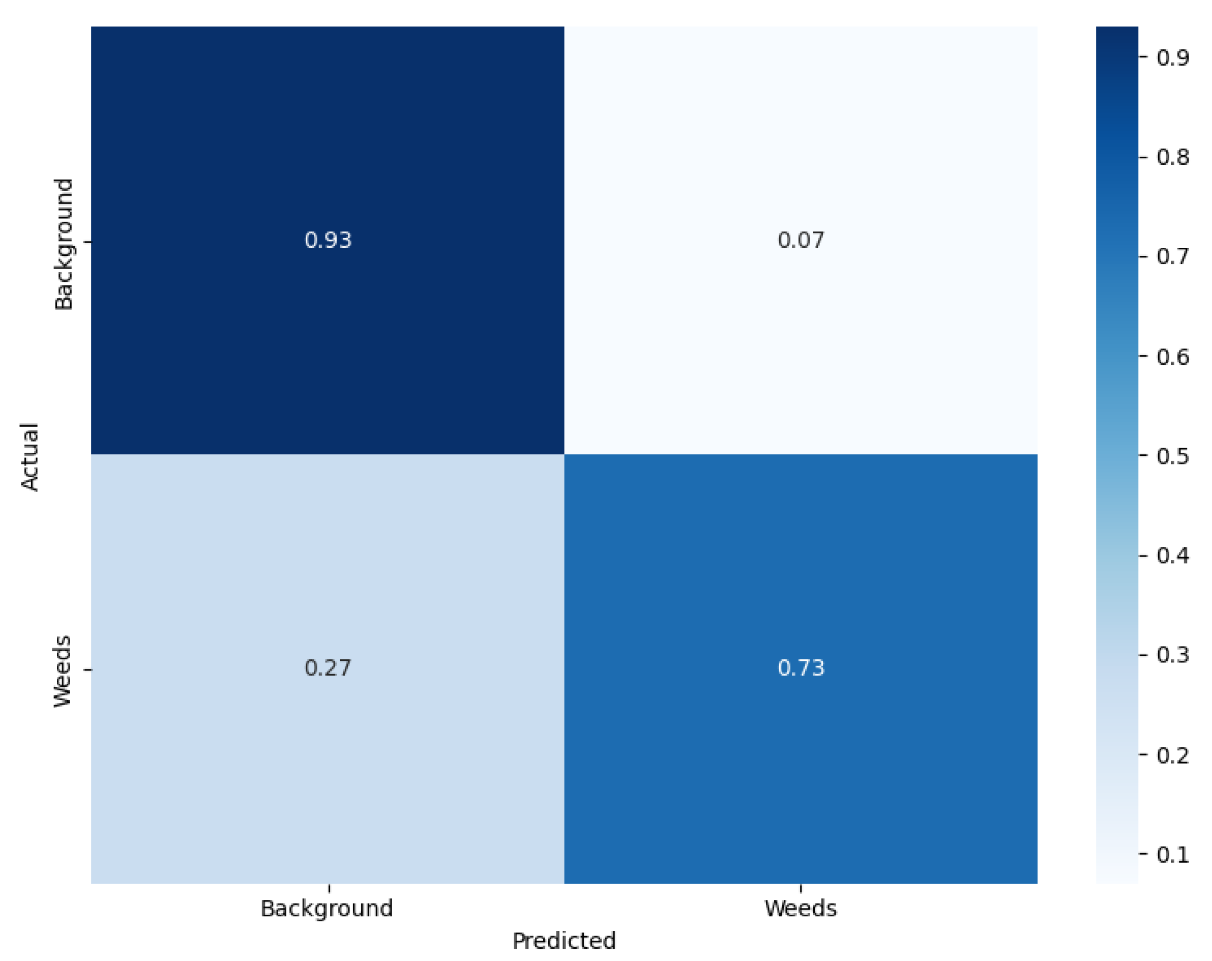
Confusion Matrix (Figure 6 and Figure 7): Summarizes true/false positives and negatives per class. Basis for precision, recall, and F1-score calculations.
Model Size: The total storage size of the trained model, expressed in megabytes (MB), indicates its memory efficiency.
Average Inference Time per Image: The average duration required to process a single image during inference, reflecting the model’s speed and usability in real-time applications.
These metrics collectively provide a holistic evaluation of segmentation performance, computational efficiency, and resource demands, ensuring a transparent and fair comparison among all evaluated models.
5. Results
5.1. Comparisons with Benchmarks on Segmentation Datasets
The proposed model is evaluated against benchmark methods across two UAV-based image segmentation datasets.
Table 3 and
Table 4 provide a comprehensive comparison of segmentation models using different backbone CNNs. The evaluation metrics include mean IoU, precision, recall, F1-score, IoU for background, crop, and weeds.
Quantitative Comparisons with Benchmarks
Table 3 and
Table 4 provide a comprehensive comparison of MSEA-Net with various benchmark models across key segmentation metrics, including mean IoU, precision, recall, F1-score, and per-class IoU scores. On the Colfy-WeedDB dataset (
Table 3), MSEA-Net achieves the highest mean IoU (71.35%), outperforming models like DenseNet121 SegNet (67.56%) and EfficientNetB0 SegNet (67.24%). It also demonstrates superior weighted precision (90.33%) and weighted recall (90.03%), reinforcing its robustness in segmentation tasks. In addition to the tabulated results, we have provided
Figure 8 and
Figure 9 for visual comparison of these metrics, further highlighting MSEA-Net’s consistent performance advantages over baseline models. The model attains an IoU of 88.72% for the background class and 53.99% for the weed class, outperforming alternative architectures in distinguishing key regions. On the Motion-Blurred UAV Images of Sorghum Fields dataset (
Table 4), MSEA-Net again achieves the highest mean IoU (87.42%), surpassing other architectures such as UNet with EfficientNetB0 (85.34%) and UNet with DenseNet121 (84.46%). It also demonstrates superior precision (93.54%), recall (92.61%), and F1-score (93.07%), highlighting its robustness in multi-class segmentation. The model performs exceptionally well in per-class segmentation, achieving an IoU of 99.19% for the background class, 84.00% for the crop class, and 79.08% for the weed class, significantly outperforming models such as SegNet with DenseNet121 (81.64%) and DeepLabV3+ with MobileNetV2 (64.55%). In terms of computational efficiency, MSEA-Net maintains only 6.74 M parameters and a model size of 25.74 MB, making it significantly more efficient than larger models such as UNet with DenseNet121 (32.56 M parameters, 124.21 MB) while delivering superior segmentation accuracy. Other architectures, including SegNet with ResNet50 (63.39% IoU) and DeepLabV3+ with DenseNet121 (62.35% IoU), show lower performance, reinforcing MSEA-Net’s effectiveness. These results establish MSEA-Net as a state-of-the-art solution, balancing high segmentation accuracy with reduced computational complexity across diverse datasets.
5.2. Statistical Validation of MESA-Net Across Multiple Folds
To validate the consistency of the MESA-Net, we provide the five-fold cross-validation results for the proposed MESA-Net on the Motion-Blurred UAV Images of Sorghum Fields [
36] dataset. The confidence interval (CI) for each performance metric is calculated at a 95% confidence level, based on Equation (
11), which offers a statistical estimate of model performance stability across the five folds [
37].
where
,
z,
, and
n represent the sample mean, confidence level, sample standard deviation, and sample size, respectively. CI was preferred over
p-values in this analysis, as relying solely on
p-values can be misleading in interpreting model performance [
38].
Table 5 reports the performance metrics across all five folds, including mean IoU, precision, recall, and F1-score. The model achieved the highest Mean IoU of 87.62% in Fold-4, with the lowest at 86.78% in Fold-3. The confidence intervals at
indicate that MESA-Net is statistically robust, with minimal variation across folds: ±0.31% for IoU, ±0.22% for precision, ±0.31% for recall, and ±0.18% for F1-score. These results highlight the consistency and reliability of MESA-Net in multi-class UAV-based weed segmentation tasks.
Examples of Visual Segmentation Results
We present visual segmentation results in
Figure 10,
Figure 11,
Figure 12 and
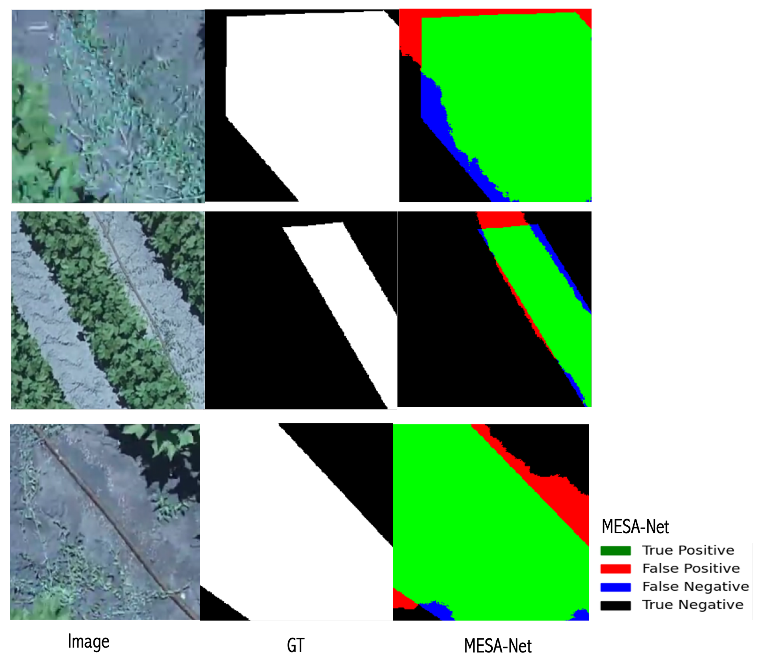
Figure 13 where we compare our model’s performance against ground truth on multiple test images. From
Figure 10, we observe that our model achieves excellent segmentation accuracy when distinguishing between weed and background in binary segmentation. Specifically, black denotes the background (true negatives), red highlights areas where the model incorrectly predicted weed as the other (false positives), green marks the correctly predicted regions of weed (true positives), and blue indicates missed regions (false negatives). The prediction overlay in this figure clearly distinguishes between green for true positives, red for false positives, and blue for false negatives, demonstrating our model’s ability to accurately separate weed and background regions. In cases where weed appears against the background, the model effectively distinguishes between them, accurately identifying weed as true positives while minimizing false positives and false negatives.
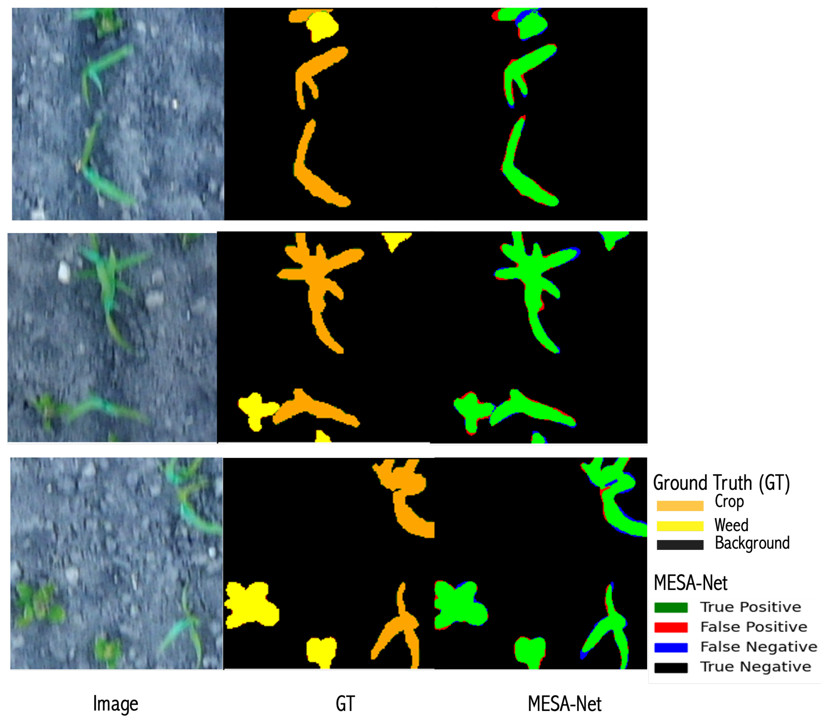
In
Figure 11, we observe a similar trend but in a multi-class segmentation scenario, where crop, weed, and background are considered distinct classes. Here, the ground truth and predicted masks are overlaid, with black denoting the background (true negatives), red highlighting the incorrect predictions for both crop and weed (false positives), and green marking the correctly predicted crop and weed regions (true positives). The prediction overlay clearly distinguishes the true positives in green, false positives in red, and false negatives in blue, demonstrating the model’s superior segmentation performance across both crop and weed classes. The model performs exceptionally well with minimal false positives and false negatives, achieving a high degree of accuracy and alignment with the ground truth. Overall, visual comparisons across both binary and multi-class segmentation tasks show that our model is robust, with highly accurate segmentation results and very few errors. Most of the observed false positives and false negatives occur in challenging regions such as shadowed areas, dense weed/crop overlaps, and regions with strong background interference.
5.3. Ablation Study
5.3.1. Effectiveness of Multi-Scale Spatial-Channel Attention (MSCA) Module
The MSCA module significantly improves segmentation performance, as demonstrated in the results in
Table 6 and
Table 7. Removing MSCA leads to a sharp decline in segmentation accuracy across both datasets. For the Colfy-WeedDB dataset (
Table 6), the mean IoU drops drastically from 71.35% (with MSCA) to 57.05% (without MSCA), showing a 14.3% decline. The IoU (Bg) decreases from 88.72% to 75.12%, and IoU (Weed) falls from 53.99% to 38.98%. Similarly, for the Motion-Blurred UAV Images of Sorghum Fields dataset (
Table 7), the mean IoU drops from 87.42% (with MSCA) to 87.22% (without MSCA), while the IoU (Weed) score decreases from 79.08% to 78.47%. When MSCA is removed selectively from either the encoder or decoder, the segmentation performance still declines but to a lesser extent. For the Colfy-WeedDB dataset, removing MSCA from the encoder reduces the mean IoU to 66.88%, while removing it from the decoder results in a mean IoU of 67.61%. Likewise, in the Motion-Blurred UAV Images of Sorghum Fields dataset, excluding MSCA from the encoder lowers the mean IoU to 87.07%, whereas its removal from the decoder reduces the mean IoU to 86.90%. These results indicate that MSCA plays a vital role in both feature extraction (encoder) and refinement (decoder) stages.
In addition to performance degradation, the removal of MSCA impacts the model’s computational efficiency. For instance, excluding MSCA in the decoder increases the parameters to 10.85 M and the model size to 41.39 MB in both datasets. This demonstrates that MSCA not only enhances segmentation accuracy but also maintains computational efficiency by preventing unnecessary model bloat.
5.3.2. Effectiveness of Edge-Enhanced Bottleneck Attention (EEBA) Module
The Edge-Enhanced Bottleneck Attention (EEBA) Module plays a crucial role in accurately delineating object boundaries. The impact of EEBA can be observed in both datasets. For the Motion-Blurred UAV Images of Sorghum Fields dataset, removing EEBA leads to a drop in the mean IoU from 87.42% to 86.51%. The IoU (Weed) decreases from 79.08% to 76.71%, demonstrating that EEBA plays an essential role in precise weed segmentation. Similarly, in Colfy-WeedDB, the mean IoU decreases from 71.35% to 68.47%, while the IoU (Weed) drops from 53.99% to 49.99%. When both MSCA and EEBA are removed together, performance degradation is more severe. For the Motion-Blurred UAV Images of Sorghum Fields dataset, the mean IoU declines to 86.75%, and IoU (Weed) drops further to 77.52%. In Colfy-WeedDB, the mean IoU falls drastically to 62.15%, with background and weed IoUs reducing to 81.22% and 43.07%, respectively. These results highlight the complementary effect of EEBA and MSCA in improving model accuracy. Despite its significant impact on performance, EEBA does not increase the model’s parameters (06.74 M) or its size (25.74 MB) across both datasets. This demonstrates that EEBA enhances boundary detection without adding computational overhead, making it a highly efficient mechanism for improving segmentation performance.
The results from both datasets clearly indicate that the MSCA module and EEBA mechanism work synergistically to enhance segmentation performance while maintaining computational efficiency. Removing MSCA results in a substantial performance drop, with particularly severe consequences in Colfy-WeedDB, where segmentation becomes significantly less accurate. The EEBA module further refines boundary detection without increasing model complexity, making it an effective lightweight enhancement. Together, these components enable MSEA-Net to achieve high accuracy in UAV-based agricultural image segmentation.
5.3.3. Computational Complexity
The computational comparison demonstrates that MSEA-Net is significantly more efficient than traditional CNN-based models. With only 6.74 M parameters and a model size of 25.74 MB, MSEA-Net is much lighter than models like VGG16 and ResNet50, which have up to 32.56 M parameters and require over 120 MB of memory. This makes MSEA-Net a strong choice for resource-constrained environments such as UAVs or embedded devices, where memory and processing power are limited. Additionally, MSEA-Net achieves an average inference time of 0.0020 s per image, comparable to faster models like MobileNetV2, which supports its use in real-time applications. In contrast, heavier models such as VGG16 and ResNet50 experience slower inference times, which may hinder their deployment in time-sensitive scenarios. Overall, MSEA-Net offers a practical balance of size, speed, and accuracy, making it well suited for efficient deployment without compromising performance.
6. Discussion
This study introduced MSEA-Net, a lightweight deep learning model specifically designed for efficient and accurate weed segmentation using UAV imagery in complex agricultural environments. The core objective of MSEA-Net was to address significant challenges prevalent in UAV-based weed segmentation tasks, including environmental variability, insufficient contextual representation, inaccurate boundary detection, and the need for real-time performance on resource-constrained platforms, all while maintaining computational efficiency suitable for UAV deployment.
On the Motion-Blurred UAV Images of Sorghum Fields dataset, MSEA-Net achieved a mean IoU of 87.42% on the test set and 88.50% on the validation set (
Table 4 and
Table 8), outperforming benchmark models such as UNet with EfficientNetB0 (85.34% IoU) and SegNet with DenseNet121 (81.64% IoU). The weed class IoU reached 79.08%, exceeding the closest baseline, which achieved 74.82% (UNet with EfficientNetB0). Cross-validation results further demonstrated generalization, with a mean IoU of 87.21 ± 0.31% and an F1-score of 93.02% ± 0.18 (
Table 5).
On the CoFly-WeedDB dataset, MSEA-Net also outperformed all baselines, achieving mean IoU of 71.35%, precision of 90.33%, and weed class IoU of 53.99% and 55.02% (
Table 3 and
Table 9). By comparison, the best-performing baseline, SegNet with DenseNet121, reached 67.56% mean IoU and 47.46% weed IoU. These results confirm that MSEA-Net achieved higher segmentation accuracy across both datasets, particularly improving weed segmentation, which is typically more challenging due to smaller object size and intra-class variability.
Ablation studies (
Table 6 and
Table 7) showed the impact of the MSCA and EEBA modules. Removing MSCA reduced mean IoU by 14.3% on CoFly-WeedDB and weed IoU by 0.61% on the Sorghum dataset. EEBA’s removal reduced weed IoU by 2.37% on Sorghum. Despite these refinements, the model remained compact with 6.74 M parameters and 25.74 MB size, and achieved average inference time of 0.002 s per image (
Table 10), confirming its suitability for real-time UAV deployment.
Failure cases were observed, as shown in
Figure 10 and
Figure 11, particularly at patch borders, in shadowed regions, and with partially visible plants, where false positives and false negatives occurred. These errors were due to loss of context at patch edges and difficulties in low-contrast segmentation. Introducing sliding window patching with overlap could mitigate such issues. In addition, class imbalance in CoFly-WeedDB affected segmentation of underrepresented weed species, even with Dice–Focal Loss, indicating a need for more balanced data.
Overall, MSEA-Net consistently outperformed baseline models across both datasets in mean IoU, precision, and weed class segmentation while maintaining computational efficiency. The combination of multi-scale attention, edge-aware refinement, and lightweight design supports its use in UAV-assisted weed detection across varied field conditions.
7. Conclusions
In this study, we proposed MSEA-Net, a lightweight and efficient deep learning-based segmentation framework for UAV-assisted weed detection, addressing key challenges such as environmental variability, weak contextual representation, and inaccurate boundary detection. The Multi-Scale Spatial-Channel Attention (MSCA) module enhances multi-level spatial feature learning, ensuring better generalization across diverse agricultural conditions while minimizing computational complexity. Additionally, the Edge-Enhanced Bottleneck Attention (EEBA) module improves boundary refinement by integrating Sobel-based edge detection, reducing weed/crop misclassification errors. The lightweight design of MSEA-Net, with reduced parameters and compact model size, enables real-time performance and suitability for deployment on resource-constrained devices such as UAVs.
Extensive evaluations on publicly available datasets demonstrated that MSEA-Net achieves superior segmentation accuracy, with a mean Intersection over Union (IoU) of 71.35% on CoFly-WeedDB and 87.42% on the Sorghum dataset, along with consistently high precision, recall, and F1-score. Furthermore, with only 6.74 M parameters, a model size of 25.74 MB, and an average inference time of 0.0020 s per image, MSEA-Net offers strong computational efficiency, making it well suited for real-time UAV deployment in resource-constrained agricultural applications.
Despite the promising results, this study has some limitations. While the proposed method achieves high accuracy, generalizing it to diverse agricultural environments remains a challenge. Future work will focus on improving robustness through self-supervised learning and domain adaptation techniques. Additionally, although MSEA-Net is optimized for real-time UAV deployment, further computational optimizations, such as model pruning and quantization, will be explored to enhance efficiency. Another limitation is the reliance on publicly available datasets, which may not fully capture real-world complexities. To address this, we plan to create a diverse UAV-acquired dataset and explore multi-modal data fusion, such as hyperspectral and thermal imaging, to improve segmentation accuracy in dynamic agricultural settings.
By advancing UAV-based weed segmentation, this research contributes to sustainable precision agriculture by enabling accurate, resource-efficient, and scalable weed management solutions. These improvements have the potential to reduce herbicide dependency and optimize crop yields, fostering a more sustainable and technology-driven approach to modern agriculture.
Author Contributions
Conceptualization, A.S., B.C. and A.A.A.; methodology, A.S. and B.C.; software, B.C., S.A.B. and X.F.; validation, B.C., A.A.A. and S.A.B.; formal analysis, B.C. and A.A.A.; investigation, B.C.; resources, B.C.; data curation, A.S., B.C., A.A.A., S.A.B. and X.F.; writing—original draft preparation, A.S.; writing—review and editing, A.S., B.C., A.A.A., S.A.B. and X.F.; visualization, S.A.B. and X.F.; supervision, B.C.; project administration, B.C.; funding acquisition, B.C. All authors have read and agreed to the published version of the manuscript.
Funding
This work was supported by the Intelligent Agricultural Machinery Innovation Research and Development Project (202301) of Hunan Province, China.
Data Availability Statement
Acknowledgments
The authors would like to express their sincere gratitude to Central South University for providing research facilities and resources. Additionally, we appreciate the insightful discussions and constructive feedback from our colleagues, which helped improve this work. We also extend our thanks to those who assisted in data collection, preprocessing, and initial analysis.
Conflicts of Interest
The authors declare that they have no known competing financial interests or personal relationships that could have appeared to influence the work reported in this paper.
References
- Chakraborty, S.; Newton, A.C. Climate change, plant diseases and food security: An overview. Plant Pathol. 2011, 60, 2–14. [Google Scholar] [CrossRef]
- Brown, M.; Antle, J.; Backlund, P.; Carr, E.; Easterling, W.; Walsh, M.; Ammann, C.; Attavanich, W.; Barrett, C.; Bellemare, M.; et al. Climate Change, Global Food Security, and the U.S. Food System; Technical Report; U.S. Global Change Research Program: Washington, DC, USA, 2015. [Google Scholar] [CrossRef]
- Berquer, A.; Bretagnolle, V.; Martin, O.; Gaba, S. Disentangling the effect of nitrogen input and weed control on crop–weed competition suggests a potential agronomic trap in conventional farming. Agric. Ecosyst. Environ. 2023, 345, 108232. [Google Scholar] [CrossRef]
- Monteiro, A.; Santos, S. Sustainable Approach to Weed Management: The Role of Precision Weed Management. Agronomy 2022, 12, 118. [Google Scholar] [CrossRef]
- Adhinata, F.D.; Wahyono; Sumiharto, R. A comprehensive survey on weed and crop classification using machine learning and deep learning. Artif. Intell. Agric. 2024, 13, 45–63. [Google Scholar] [CrossRef]
- Mohsan, S.A.H.; Othman, N.Q.H.; Li, Y.; Alsharif, M.H.; Khan, M.A. Unmanned aerial vehicles (UAVs): Practical aspects, applications, open challenges, security issues, and future trends. Intell. Serv. Robot. 2023, 16, 109–137. [Google Scholar] [CrossRef]
- Sachithra, V.; Subhashini, L.D. How artificial intelligence uses to achieve the agriculture sustainability: Systematic review. Artif. Intell. Agric. 2023, 8, 46–59. [Google Scholar] [CrossRef]
- Sapkota, R.; Ahmed, D.; Karkee, M. Comparing YOLOv8 and Mask R-CNN for instance segmentation in complex orchard environments. Artif. Intell. Agric. 2024, 13, 84–99. [Google Scholar] [CrossRef]
- Zhang, J.; Maleski, J.; Jespersen, D.; Waltz, F.C.; Rains, G.; Schwartz, B. Unmanned Aerial System-Based Weed Mapping in Sod Production Using a Convolutional Neural Network. Front. Plant Sci. 2021, 12, 702626. [Google Scholar] [CrossRef]
- Moazzam, S.I.; Khan, U.S.; Qureshi, W.S.; Nawaz, T.; Kunwar, F. Towards automated weed detection through two-stage semantic segmentation of tobacco and weed pixels in aerial Imagery. Smart Agric. Technol. 2023, 4, 100142. [Google Scholar] [CrossRef]
- Sivakumar, A.N.V.; Li, J.; Scott, S.; Psota, E.; Jhala, A.J.; Luck, J.D.; Shi, Y. Comparison of Object Detection and Patch-Based Classification Deep Learning Models on Mid- to Late-Season Weed Detection in UAV Imagery. Remote Sens. 2020, 12, 2136. [Google Scholar] [CrossRef]
- Sunil, G.C.; Koparan, C.; Ahmed, M.R.; Zhang, Y.; Howatt, K.; Sun, X. A study on deep learning algorithm performance on weed and crop species identification under different image background. Artif. Intell. Agric. 2022, 6, 242–256. [Google Scholar] [CrossRef]
- Vasileiou, M.; Kyrgiakos, L.S.; Kleisiari, C.; Kleftodimos, G.; Vlontzos, G.; Belhouchette, H.; Pardalos, P.M. Transforming weed management in sustainable agriculture with artificial intelligence: A systematic literature review towards weed identification and deep learning. Crop Prot. 2024, 176, 106522. [Google Scholar] [CrossRef]
- Upadhyay, A.; Zhang, Y.; Koparan, C.; Rai, N.; Howatt, K.; Bajwa, S.; Sun, X. Advances in ground robotic technologies for site-specific weed management in precision agriculture: A review. Comput. Electron. Agric. 2024, 225, 109363. [Google Scholar] [CrossRef]
- Nathalie, C.; Munier-Jolain, N.; Dugué, F.; Gardarin, A.; Strbik, F.; Moreau, D. The response of weed and crop species to shading. How to predict their morphology and plasticity from species traits and ecological indexes? Eur. J. Agron. 2020, 121, 126158. [Google Scholar] [CrossRef]
- Sabzi, S.; Abbaspour-Gilandeh, Y.; Arribas, J.I. An automatic visible-range video weed detection, segmentation and classification prototype in potato field. Heliyon 2020, 6, e03685. [Google Scholar] [CrossRef]
- Subeesh, A.; Bhole, S.; Singh, K.; Chandel, N.S.; Rajwade, Y.A.; Rao, K.V.; Kumar, S.P.; Jat, D. Deep convolutional neural network models for weed detection in polyhouse grown bell peppers. Artif. Intell. Agric. 2022, 6, 47–54. [Google Scholar] [CrossRef]
- Gallo, I.; Rehman, A.U.; Dehkordi, R.H.; Landro, N.; Grassa, R.L.; Boschetti, M. Deep Object Detection of Crop Weeds: Performance of YOLOv7 on a Real Case Dataset from UAV Images. Remote Sens. 2023, 15, 539. [Google Scholar] [CrossRef]
- Shahi, T.B.; Dahal, S.; Sitaula, C.; Neupane, A.; Guo, W. Deep Learning-Based Weed Detection Using UAV Images: A Comparative Study. Drones 2023, 7, 624. [Google Scholar] [CrossRef]
- Fathipoor, H.; Shah-Hosseini, R.; Arefi, H. Crop and Weed Segmentation on Ground-Based Images Using Deep Convolutional Neural Network. ISPRS Ann. Photogramm. Remote Sens. Spat. Inf. Sci. 2023, 10, 195–200. [Google Scholar] [CrossRef]
- dos Santos Ferreira, A.; Freitas, D.M.; da Silva, G.G.; Pistori, H.; Folhes, M.T. Weed detection in soybean crops using ConvNets. Comput. Electron. Agric. 2017, 143, 314–324. [Google Scholar] [CrossRef]
- Razfar, N.; True, J.; Bassiouny, R.; Venkatesh, V.; Kashef, R. Weed detection in soybean crops using custom lightweight deep learning models. J. Agric. Food Res. 2022, 8, 100308. [Google Scholar] [CrossRef]
- Ong, P.; Teo, K.S.; Sia, C.K. UAV-based weed detection in Chinese cabbage using deep learning. Smart Agric. Technol. 2023, 4, 100181. [Google Scholar] [CrossRef]
- Xu, B.; Fan, J.; Chao, J.; Arsenijevic, N.; Werle, R.; Zhang, Z. Instance segmentation method for weed detection using UAV imagery in soybean fields. Comput. Electron. Agric. 2023, 211, 107994. [Google Scholar] [CrossRef]
- Ullah, H.S.; Bais, A. Evaluation of model generalization for growing plants using conditional learning. Artif. Intell. Agric. 2022, 6, 189–198. [Google Scholar] [CrossRef]
- Bah, M.D.; Hafiane, A.; Canals, R. Deep Learning with Unsupervised Data Labeling for Weed Detection in Line Crops in UAV Images. Remote Sens. 2018, 10, 1690. [Google Scholar] [CrossRef]
- Lin, J.; Zhang, X.; Qin, Y.; Yang, S.; Wen, X.; Cernava, T.; Chen, X. FG-UNet: Fine-grained feature-guided UNet for segmentation of weeds and crops in UAV images. Pest Manag. Sci. 2024, 81, 856–866. [Google Scholar] [CrossRef]
- Zou, K.; Chen, X.; Zhang, F.; Zhou, H.; Zhang, C. A Field Weed Density Evaluation Method Based on UAV Imaging and Modified U-Net. Remote Sens. 2021, 13, 310. [Google Scholar] [CrossRef]
- Gao, J.; Liao, W.; Nuyttens, D.; Lootens, P.; Xue, W.; Alexandersson, E.; Pieters, J. Cross-domain transfer learning for weed segmentation and mapping in precision farming using ground and UAV images. Expert Syst. Appl. 2024, 246, 122980. [Google Scholar] [CrossRef]
- Machidon, A.L.; Krasovec, A.; Pejovic, V.; Machidon, O.M. SqueezeSlimU-Net: An Adaptive and Efficient Segmentation Architecture for Real-Time UAV Weed Detection. IEEE J. Sel. Top. Appl. Earth Obs. Remote Sens. 2025, 18, 5749–5764. [Google Scholar] [CrossRef]
- Zhao, H.; Shi, J.; Qi, X.; Wang, X.; Jia, J. Pyramid scene parsing network. In Proceedings of the 30th IEEE Conference on Computer Vision and Pattern Recognition, CVPR 2017, Honolulu, HI, USA, 21–26 July 2017; pp. 6230–6239. [Google Scholar] [CrossRef]
- Kuang, H.; Menon, B.K.; Sohn, S.I.; Qiu, W. EIS-Net: Segmenting early infarct and scoring ASPECTS simultaneously on non-contrast CT of patients with acute ischemic stroke. Med. Image Anal. 2021, 70, 101984. [Google Scholar] [CrossRef]
- Chen, L.C.; Zhu, Y.; Papandreou, G.; Schroff, F.; Adam, H. Encoder-decoder with atrous separable convolution for semantic image segmentation. In Proceedings of the European Conference on Computer Vision (ECCV), Munich, Germany, 8–14 September 2018; pp. 801–818. [Google Scholar] [CrossRef]
- Hu, J.; Shen, L.; Sun, G. Squeeze-and-Excitation Networks. In Proceedings of the IEEE Conference on Computer Vision and Pattern Recognition, Salt Lake City, UT, USA, 18–22 June 2018. [Google Scholar]
- Krestenitis, M.; Raptis, E.K.; Kapoutsis, A.C.; Ioannidis, K.; Kosmatopoulos, E.B.; Vrochidis, S.; Kompatsiaris, I. CoFly-WeedDB: A UAV image dataset for weed detection and species identification. Data Brief 2022, 45, 108575. [Google Scholar] [CrossRef] [PubMed]
- Genze, N.; Ajekwe, R.; Güreli, Z.; Haselbeck, F.; Grieb, M.; Grimm, D.G. Deep learning-based early weed segmentation using motion blurred UAV images of sorghum fields. Comput. Electron. Agric. 2022, 202, 107388. [Google Scholar] [CrossRef]
- Dekking, F.M.; Kraaikamp, C.; Lopuhaä, H.P.; Meester, L.E. A Modern Introduction to Probability and Statistics; Springer: Berlin/Heidelberg, Germany, 2005. [Google Scholar] [CrossRef]
- Pandis, N. Confidence intervals rather than P values. Am. J. Orthod. Dentofac. Orthop. 2013, 143, 293–294. [Google Scholar] [CrossRef] [PubMed]
Figure 1.
Proposed MSEA-Net: A hierarchical encoder–decoder network that integrates Multi-Scale Spatial-Channel Attention (MSCA) and Edge-Enhanced Bottleneck Attention (EEBA) modules, leveraging spatial and channel attention to efficiently extract and refine features for accurate image segmentation.
Figure 2.
Multi-Scale Spatial-Channel Attention (MSCA) Module: Captures and fuses multi-scale features using hierarchical convolutions, spatial attention (SPA), and squeeze-and-excitation (SE) blocks.
Figure 2.
Multi-Scale Spatial-Channel Attention (MSCA) Module: Captures and fuses multi-scale features using hierarchical convolutions, spatial attention (SPA), and squeeze-and-excitation (SE) blocks.
Figure 3.
Edge-Enhanced Bottleneck Attention (EEBA) module: Extracts and fuses edge-aware and spatial features to enhance bottleneck representation for decoding.
Figure 3.
Edge-Enhanced Bottleneck Attention (EEBA) module: Extracts and fuses edge-aware and spatial features to enhance bottleneck representation for decoding.
Figure 4.
Spatial Attention Module: Combines pointwise convolutions, ReLU activation, and spatial gating with residual connections to enhance spatial dependencies.
Figure 4.
Spatial Attention Module: Combines pointwise convolutions, ReLU activation, and spatial gating with residual connections to enhance spatial dependencies.
Figure 5.
Squeeze-and-excitation (SE) block: Enhances channel dependencies by emphasizing significant features.
Figure 5.
Squeeze-and-excitation (SE) block: Enhances channel dependencies by emphasizing significant features.
Figure 6.
Confusion matrix for MSEA-Net on the CoFly-WeedDB. The matrix shows class-wise prediction accuracy for background and weed classes, highlighting the model’s ability to minimize misclassification under imbalanced data conditions.
Figure 6.
Confusion matrix for MSEA-Net on the CoFly-WeedDB. The matrix shows class-wise prediction accuracy for background and weed classes, highlighting the model’s ability to minimize misclassification under imbalanced data conditions.
Figure 7.
Confusion matrix for MSEA-Net on the Sorghum dataset. The matrix illustrates prediction accuracy across background, crop, and weed classes, demonstrating effective multi-class segmentation performance with low error rates.
Figure 7.
Confusion matrix for MSEA-Net on the Sorghum dataset. The matrix illustrates prediction accuracy across background, crop, and weed classes, demonstrating effective multi-class segmentation performance with low error rates.
Figure 8.
Performance comparison of MESA-Net and various backbone CNNs on the Colfy-WeedDB. MESA-Net outperforms other models in terms of mean IoU, precision, recall, and F1-score, indicating its superior capability for weed segmentation tasks.
Figure 8.
Performance comparison of MESA-Net and various backbone CNNs on the Colfy-WeedDB. MESA-Net outperforms other models in terms of mean IoU, precision, recall, and F1-score, indicating its superior capability for weed segmentation tasks.
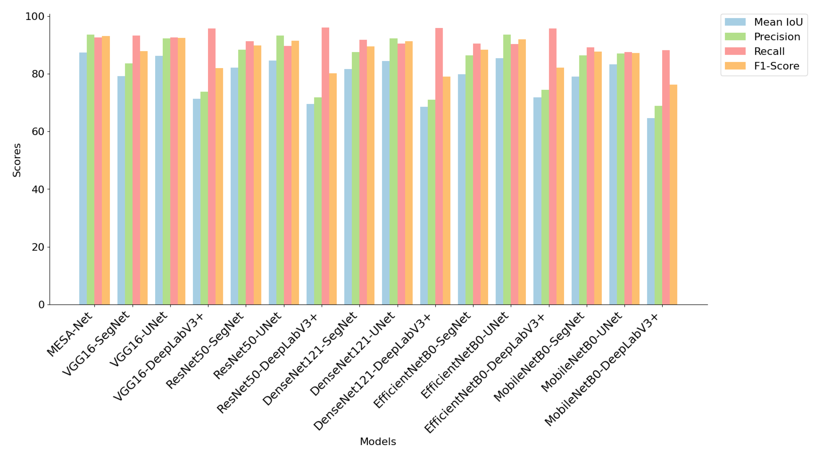
Figure 9.
Performance comparison of MESA-Net and various backbone CNNs on the Motion-Blurred UAV Images of Sorghum Fields dataset. MESA-Net outperforms other models in terms of mean IoU, precision, recall, and F1-score, indicating its superior capability for weed segmentation tasks.
Figure 9.
Performance comparison of MESA-Net and various backbone CNNs on the Motion-Blurred UAV Images of Sorghum Fields dataset. MESA-Net outperforms other models in terms of mean IoU, precision, recall, and F1-score, indicating its superior capability for weed segmentation tasks.
Figure 10.
Visual segmentation results for weed detection in a binary segmentation scenario, distinguishing between weed and background. True positives are in green, false positives in red, and false negatives in blue, with MSEA-Net demonstrating excellent accuracy and minimal errors.
Figure 10.
Visual segmentation results for weed detection in a binary segmentation scenario, distinguishing between weed and background. True positives are in green, false positives in red, and false negatives in blue, with MSEA-Net demonstrating excellent accuracy and minimal errors.
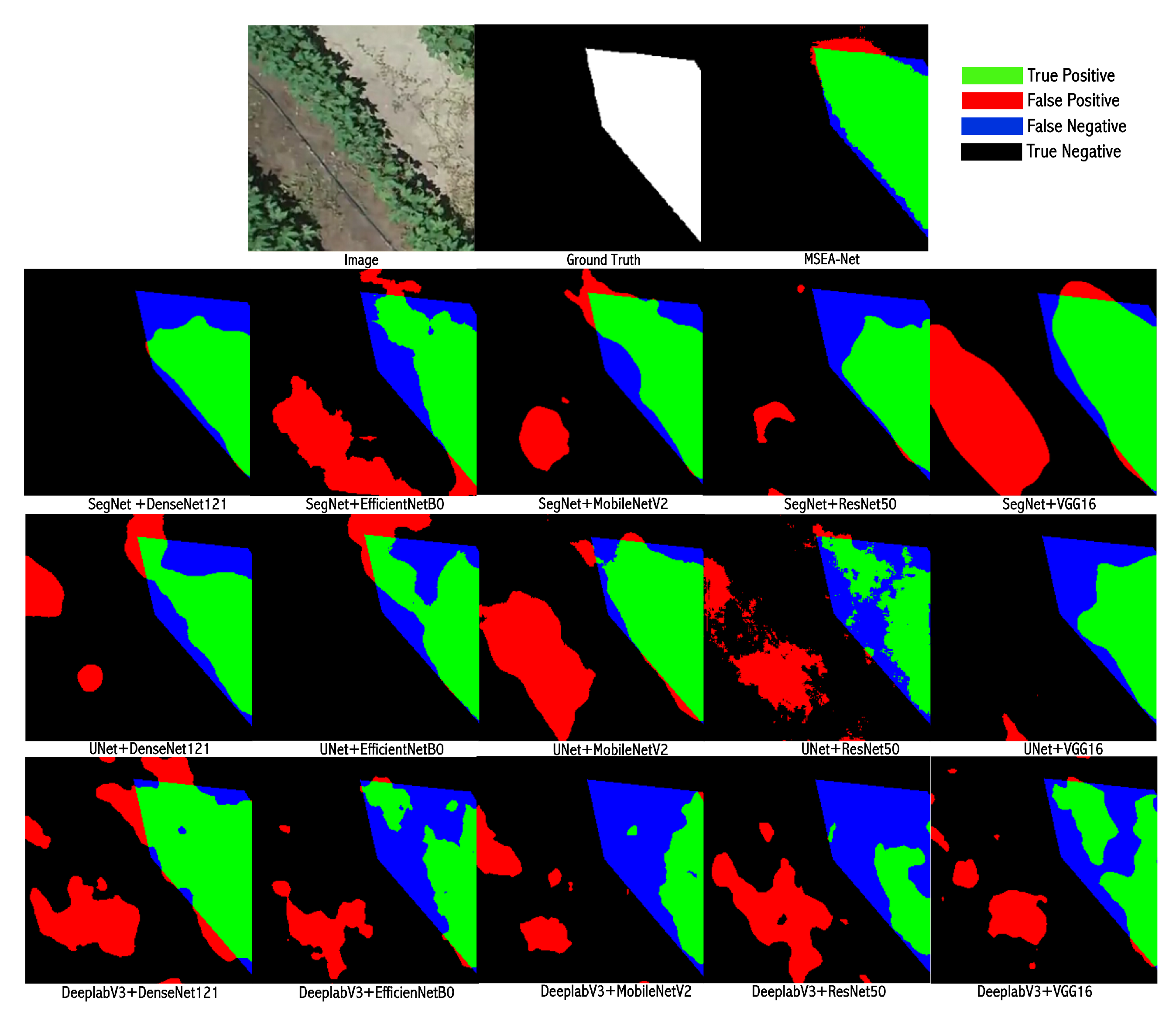
Figure 11.
Visual segmentation results in a multi-class scenario, where crop, weed, and background are considered distinct classes. True positives are in green, false positives in red, and false negatives in blue, with MSEA-Net demonstrating superior performance and minimal errors across all classes.
Figure 12.
Visual segmentation results for weed detection in a binary segmentation scenario.
Figure 12.
Visual segmentation results for weed detection in a binary segmentation scenario.
Figure 13.
Visual segmentation results in a multi-class scenario.
Figure 13.
Visual segmentation results in a multi-class scenario.
Table 1.
Dataset overview.
Table 1.
Dataset overview.
| Dataset | Original Images | Patches | Weed Threshold |
|---|
| (Resolution) | (256 × 256) | (Augmentations) |
|---|
| CoFly-WeedDB [35] | 201 images | 786 | Min. 3% weed |
| (1280 × 720) | (Flip, Rotation, Grid Distortion) |
| Motion-Blurred UAV Images of Sorghum Fields [36] | 19 images | 6300 | Min. 3% weed |
| (5472 × 3648) | (Flip, Rotation, Grid Distortion) |
Table 2.
Hyperparameter settings.
Table 2.
Hyperparameter settings.
| Hyperparameter | Value |
|---|
| Epochs | 200 |
| Learning Rate (LR) | 0.002 |
| Batch Size | 64 |
| Patience | 20 |
| Optimizer | Adam |
Table 3.
Comparative evaluation of MESA-Net and backbone CNNs on Colfy-WeedDB dataset (testing set).
Table 3.
Comparative evaluation of MESA-Net and backbone CNNs on Colfy-WeedDB dataset (testing set).
| Backbone CNN | Model | Mean IoU | Precision | Recall | F1-Score | IoU (Bg) | IoU (Weed) |
|---|
| VGG16 | SegNet | 65.38 | 88.26 | 85.23 | 86.20 | 86.25 | 46.60 |
| UNet | 64.22 | 87.09 | 88.06 | 87.12 | 86.28 | 41.03 |
| DeepLabV3+ | 61.56 | 85.15 | 85.92 | 85.45 | 79.31 | 37.75 |
| ResNet50 | SegNet | 63.39 | 86.06 | 86.55 | 86.27 | 85.90 | 46.29 |
| UNet | 65.57 | 87.48 | 88.32 | 87.63 | 87.15 | 43.20 |
| DeepLabV3+ | 63.57 | 86.13 | 86.40 | 86.26 | 84.68 | 40.30 |
| DenseNet121 | SegNet | 67.56 | 88.26 | 88.90 | 88.43 | 87.66 | 47.46 |
| UNet | 67.13 | 87.97 | 88.56 | 88.17 | 87.10 | 46.06 |
| DeepLabV3+ | 62.35 | 85.61 | 85.21 | 85.40 | 81.52 | 41.88 |
| EfficientNetB0 | SegNet | 67.24 | 87.95 | 87.88 | 87.92 | 85.25 | 47.11 |
| UNet | 66.72 | 87.82 | 88.47 | 88.02 | 87.09 | 46.40 |
| DeepLabV3+ | 61.84 | 85.53 | 86.63 | 85.82 | 81.81 | 35.41 |
| MobileNetV2 | SegNet | 64.06 | 87.52 | 84.58 | 85.56 | 87.10 | 45.06 |
| UNet | 65.42 | 87.06 | 87.47 | 87.24 | 84.02 | 47.21 |
| DeepLabV3+ | 59.87 | 84.25 | 85.16 | 84.61 | 84.35 | 27.17 |
| MESA-Net | MESA-Net | 71.35 | 90.33 | 90.03 | 90.17 | 88.72 | 53.99 |
Table 4.
Comparative evaluation of MESA-Net and backbone CNNs on Motion-Blurred UAV Images of Sorghum Fields dataset (testing set).
Table 4.
Comparative evaluation of MESA-Net and backbone CNNs on Motion-Blurred UAV Images of Sorghum Fields dataset (testing set).
| Backbone CNN | Model | Mean IoU | Precision | Recall | F1-Score | IoU (Bg) | IoU (Crop) | IoU (Weed) |
|---|
| VGG16 | SegNet | 79.12 | 83.52 | 93.23 | 87.86 | 97.62 | 74.69 | 65.05 |
| UNet | 86.15 | 92.23 | 92.58 | 92.40 | 98.60 | 82.83 | 77.01 |
| DeepLabV3+ | 71.25 | 73.71 | 95.65 | 81.94 | 96.30 | 68.52 | 48.93 |
| ResNet50 | SegNet | 82.04 | 88.40 | 91.26 | 89.79 | 98.14 | 78.22 | 69.75 |
| UNet | 84.52 | 93.23 | 89.71 | 91.38 | 98.49 | 81.09 | 74.02 |
| DeepLabV3+ | 69.43 | 71.77 | 96.00 | 80.21 | 95.96 | 69.64 | 42.70 |
| DenseNet121 | SegNet | 81.64 | 87.56 | 91.69 | 89.54 | 98.08 | 77.67 | 69.19 |
| UNet | 84.46 | 92.33 | 90.40 | 91.34 | 98.52 | 81.14 | 73.73 |
| DeepLabV3+ | 68.50 | 70.94 | 95.90 | 79.00 | 95.81 | 72.27 | 37.41 |
| EfficientNetB0 | SegNet | 79.90 | 86.44 | 90.46 | 88.37 | 97.87 | 75.88 | 65.96 |
| UNet | 85.34 | 93.62 | 90.27 | 91.88 | 98.60 | 82.59 | 74.82 |
| DeepLabV3+ | 71.86 | 74.39 | 95.66 | 82.16 | 96.68 | 72.06 | 68.30 |
| MobileNetV2 | SegNet | 78.96 | 86.30 | 89.21 | 87.71 | 97.84 | 74.70 | 64.33 |
| UNet | 83.27 | 87.06 | 87.47 | 87.24 | 84.02 | 47.21 | 70.54 |
| DeepLabV3+ | 64.55 | 68.81 | 88.23 | 76.22 | 95.48 | 60.38 | 37.78 |
| MESA-Net | MESA-Net | 87.42 | 93.54 | 92.61 | 93.07 | 99.19 | 84.00 | 79.08 |
Table 5.
Five-fold cross-validation performance of MESA-Net on Motion-Blurred UAV Images of Sorghum Fields dataset.
Table 5.
Five-fold cross-validation performance of MESA-Net on Motion-Blurred UAV Images of Sorghum Fields dataset.
| Fold | Mean IoU | Precision | Recall | F1-Score |
|---|
| Fold-1 | 86.91 | 93.12 | 92.30 | 92.75 |
| Fold-2 | 87.42 | 93.54 | 92.61 | 93.07 |
| Fold-3 | 86.78 | 93.41 | 92.18 | 92.89 |
| Fold-4 | 87.62 | 93.67 | 92.89 | 93.22 |
| Fold-5 | 87.33 | 93.68 | 92.93 | 93.17 |
| CI | 87.21 ± 0.31 | 93.48 ± 0.22 | 92.58 ± 0.31 | 93.02 ± 0.18 |
Table 6.
Ablation study results on Colfy-WeedDB dataset.
Table 6.
Ablation study results on Colfy-WeedDB dataset.
| Method | Mean IoU | IoU (Bg) | IoU (Weed) | Param (M) | Model Size (MB) |
|---|
| MEA-Net | 71.35 | 88.72 | 53.99 | 06.74 | 25.74 |
| w/o MSCA | 57.05 | 75.12 | 38.98 | 10.49 | 40.05 |
| w/o EEBA | 68.47 | 86.94 | 49.99 | 6.74 | 25.74 |
| w/o MSCA in Enc | 66.88 | 84.71 | 48.99 | 06.39 | 24.40 |
| w/o MSCA in Dec | 67.61 | 85.57 | 49.56 | 10.85 | 41.39 |
| w/o MSCA & EEBA | 62.15 | 81.22 | 43.07 | 09.60 | 36.63 |
Table 7.
Ablation study results on Motion-Blurred UAV Images of Sorghum Fields dataset.
Table 7.
Ablation study results on Motion-Blurred UAV Images of Sorghum Fields dataset.
| Method | Mean IoU | IoU (Bg) | IoU (Crop) | IoU (Weed) | Param (M) | Model Size (MB) |
|---|
| MEA-Net | 87.42 | 99.19 | 84.00 | 79.08 | 06.74 | 25.74 |
| w/o MSCA | 87.22 | 99.18 | 84.00 | 78.47 | 10.49 | 40.05 |
| w/o EEBA | 86.51 | 99.18 | 83.62 | 76.71 | 06.74 | 25.74 |
| w/o MSCA in Enc | 87.07 | 99.19 | 84.33 | 77.69 | 06.39 | 24.40 |
| w/o MSCA in Dec | 86.90 | 99.19 | 83.63 | 77.55 | 10.85 | 41.39 |
| w/o MSCA & EEBA | 86.75 | 99.18 | 83.55 | 77.52 | 09.60 | 36.63 |
Table 8.
Comparative evaluation of MESA-Net and backbone CNNs on Motion-Blurred UAV Images of Sorghum Fields dataset (validation set).
Table 8.
Comparative evaluation of MESA-Net and backbone CNNs on Motion-Blurred UAV Images of Sorghum Fields dataset (validation set).
| Backbone CNN | Model | Mean IoU | Precision | Recall | F1-Score | IoU (Bg) | IoU (Crop) | IoU (Weed) |
|---|
| VGG16 | SegNet | 80.05 | 84.20 | 94.00 | 88.45 | 97.92 | 75.45 | 66.30 |
| UNet | 86.90 | 92.80 | 93.15 | 92.97 | 98.85 | 83.30 | 78.05 |
| DeepLabV3+ | 72.40 | 74.20 | 96.10 | 82.35 | 96.65 | 69.20 | 50.05 |
| ResNet50 | SegNet | 83.00 | 89.10 | 92.00 | 90.52 | 98.40 | 79.05 | 71.00 |
| UNet | 85.20 | 93.80 | 90.50 | 92.10 | 98.75 | 81.90 | 75.00 |
| DeepLabV3+ | 70.15 | 72.60 | 96.35 | 81.05 | 96.20 | 70.45 | 44.15 |
| DenseNet121 | SegNet | 82.40 | 88.30 | 92.25 | 90.20 | 98.30 | 78.90 | 70.50 |
| UNet | 85.00 | 92.85 | 91.10 | 91.97 | 98.70 | 81.85 | 74.50 |
| DeepLabV3+ | 69.30 | 72.00 | 96.00 | 80.50 | 96.10 | 73.05 | 39.70 |
| EfficientNetB0 | SegNet | 80.80 | 87.00 | 91.00 | 89.00 | 98.10 | 76.75 | 67.20 |
| UNet | 86.00 | 94.00 | 91.00 | 92.50 | 98.85 | 83.00 | 75.50 |
| DeepLabV3+ | 73.20 | 75.10 | 96.00 | 83.00 | 97.10 | 73.55 | 69.50 |
| MobileNetV2 | SegNet | 79.80 | 87.00 | 90.00 | 88.40 | 98.00 | 75.80 | 66.00 |
| UNet | 84.20 | 88.50 | 88.90 | 88.70 | 84.50 | 49.00 | 72.00 |
| DeepLabV3+ | 65.80 | 70.00 | 89.50 | 77.50 | 95.90 | 62.75 | 39.30 |
| MESA-Net | MESA-Net | 88.28 | 94.03 | 93.12 | 93.55 | 99.40 | 85.10 | 80.34 |
Table 9.
Comparative evaluation of MESA-Net and backbone CNNs on Colfy-WeedDB dataset (validation set).
Table 9.
Comparative evaluation of MESA-Net and backbone CNNs on Colfy-WeedDB dataset (validation set).
| Backbone CNN | Model | Mean IoU | Precision | Recall | F1-Score | IoU (Bg) | IoU (Weed) |
|---|
| VGG16 | SegNet | 66.45 | 88.92 | 85.80 | 86.75 | 87.02 | 47.88 |
| UNet | 65.78 | 87.85 | 88.65 | 88.24 | 86.91 | 42.76 |
| DeepLabV3+ | 62.93 | 86.10 | 86.75 | 86.42 | 80.15 | 38.65 |
| ResNet50 | SegNet | 64.82 | 87.01 | 87.30 | 87.15 | 86.72 | 47.10 |
| UNet | 66.32 | 88.10 | 88.90 | 88.50 | 88.02 | 44.85 |
| DeepLabV3+ | 64.00 | 86.72 | 87.01 | 86.86 | 85.50 | 41.30 |
| DenseNet121 | SegNet | 68.12 | 89.02 | 89.35 | 89.18 | 88.30 | 48.56 |
| UNet | 67.80 | 88.75 | 89.10 | 88.92 | 87.90 | 47.72 |
| DeepLabV3+ | 63.58 | 86.20 | 85.85 | 86.02 | 82.05 | 42.95 |
| EfficientNetB0 | SegNet | 67.88 | 88.55 | 88.30 | 88.42 | 86.01 | 48.35 |
| UNet | 67.35 | 88.25 | 88.90 | 88.57 | 88.10 | 47.88 |
| DeepLabV3+ | 62.49 | 86.10 | 87.20 | 86.64 | 82.95 | 36.87 |
| MobileNetV2 | SegNet | 65.10 | 88.00 | 85.23 | 86.45 | 87.50 | 46.05 |
| UNet | 66.00 | 87.72 | 88.00 | 87.86 | 85.12 | 48.55 |
| DeepLabV3+ | 60.32 | 85.00 | 85.75 | 85.37 | 85.10 | 28.55 |
| MESA-Net | MESA-Net | 72.50 | 91.10 | 90.80 | 90.94 | 89.55 | 55.02 |
Table 10.
Computational complexity.
Table 10.
Computational complexity.
| Backbone CNN | Model | Param (M) | Model Size (MB) | Avg Inference Time (s) |
|---|
| VGG16 | SegNet | 24.72 | 92.29 | 0.0029 |
| UNet | 23.75 | 90.61 | 0.0018 |
| DeepLabV3+ | 09.86 | 37.50 | 0.0014 |
| ResNet50 | SegNet | 20.95 | 79.93 | 0.0025 |
| UNet | 32.56 | 124.21 | 0.0019 |
| DeepLabV3+ | 03.68 | 14.04 | 0.0017 |
| DenseNet121 | SegNet | 14.85 | 56.65 | 0.0026 |
| UNet | 12.15 | 46.33 | 0.0020 |
| DeepLabV3+ | 03.53 | 13.48 | 0.0017 |
| EfficientNetB0 | SegNet | 10.21 | 38.96 | 0.0024 |
| UNet | 10.12 | 38.59 | 0.0014 |
| DeepLabV3+ | 02.20 | 8.38 | 0.0016 |
| MobileNetV2 | SegNet | 10.91 | 41.63 | 0.0023 |
| UNet | 08.05 | 30.70 | 0.0012 |
| DeepLabV3+ | 02.17 | 08.28 | 0.0014 |
| MESA-Net | MESA-Net | 06.74 | 25.74 | 0.0020 |
| Disclaimer/Publisher’s Note: The statements, opinions and data contained in all publications are solely those of the individual author(s) and contributor(s) and not of MDPI and/or the editor(s). MDPI and/or the editor(s) disclaim responsibility for any injury to people or property resulting from any ideas, methods, instructions or products referred to in the content. |
© 2025 by the authors. Licensee MDPI, Basel, Switzerland. This article is an open access article distributed under the terms and conditions of the Creative Commons Attribution (CC BY) license (https://creativecommons.org/licenses/by/4.0/).


