Optimization and Experiment of a Subsoiling Mechanism for Hilly and Mountainous Farmland Based on the Discrete Element Method

Abstract

In response to the poor soil loosening effect of the previous bionic four-bar deep loosening mechanism, this study optimized the bionic motion trajectory according to agronomic requirements, established a trajectory synthesis optimization model of the Stephenson III six-bar mechanism, and solved it using an improved differential evolution algorithm to design a six-bar deep loosening mechanism achieving the optimized trajectory. Based on the Box–Behnken experiment, a regression model of the mechanism’s process parameters and performance indicators was established, and multiple indicators were integrated into a single objective via a satisfaction function. The optimal process parameters obtained were: entry angle 99.61°, shovel distance 185 mm, forward speed 0.29 $\mathrm{m}/\mathrm{s}$, and input speed $5\pi$ rad/s. A comparative simulation using the Discrete Element Method (DEM) showed that, compared to the bionic four-bar mechanism, the six-bar mechanism reduces resistance by 9.91%, increases soil-breaking capacity by 4.23%, reduces shallow disturbance by 14.43%, increases deep disturbance by 29.54%, and improves overall disturbance effect by 42.71%, verifying the effectiveness of agronomic-driven bionic trajectory optimization. Indoor soil tank experiments measured an average resistance of 258.83 N, with a relative error of 8.67% compared to the simulation result (281.32 N). The experiments and simulations were consistent in soil-breaking layer range, soil layer disturbance range, and soil discharge state, validating the model and the six-bar deep loosening mechanism.

1. Introduction

The hilly and mountainous farmland in China accounts for 66% of the total arable land resources. The mechanized tillage method is mainly based on small rotary tiller. The operation method for ploughing shallow soil layers can affect the soil particle structure, promoting the intensification of water erosion and wind erosion. In addition, the widespread application of pesticides and fertilizers has worsened soil compaction, coupled with the continuous compaction to the soil by traditional tillage tools [1]. The deep and medium-depth soil below 150–200 mm from the surface has evolved into a solid, thick, and hard plough pan, which greatly reduces soil porosity and seriously hinders the smooth infiltration of water and gases in the soil [2].

Xue et al. [3] designed a suspended small subsoiling machine that can control the angle between the adjustment plate and the ground to adjust the tillage depth, with a maximum depth of up to 300 mm. This design must be used in conjunction with a tractor. Hu et al. [4] designed a handheld self-propelled small subsoiling machine, powered by a horizontal bar diesel engine and relying on a tracked walking mechanism for subsoiling. There is very little research on active walking type subsoiling machines that are disconnected from traction power. It is necessary to develop small-sized subsoiling equipment suitable for hilly and mountainous farmlands with low tillage resistance and with a good soil disturbance effect.

We have combined functional biomimetic methods to design a four-bar subsoiling mechanism that can reproduce the excavation trajectory of moles [5,6]. It was found that, although the mechanism has obvious advantages in comprehensive tillage performance, its soil disturbance effect is still not good. This study optimized the biomimetic trajectory based on subsoiling agronomy as the improved subsoiling trajectory and designs a new subsoiling mechanism that has better tillage performance.

Linkage mechanism path synthesis can be transformed into nonlinear mathematical programming and solved using intelligent optimization algorithms. Acharyya et al. [7] used the Genetic Algorithm (GA), Differential Evolution (DE), and Particle Swarm Optimization (PSO) algorithms to solve the path synthesis without prescribed timing, with 10 target trajectory points in a four-bar mechanism. The results showed that DE had the smallest solution error for high-dimensional synthesis tasks. Peñuñuri et al. [8] used DE to complete path synthesis with prescribed timing for a four-bar mechanism with 18 target trajectory points. Cabrera et al. [9] used GA to complete path synthesis without prescribed timing for six target track points. Bulatović et al. [10] took the given path as a combination of a rectilinear segment and a circular arc as the target trajectory. By controlling decreases in allowed deviations, a six-bar mechanism was obtained to realize satisfactory motion. Shiakolas et al. [11] presented a methodology that combines Differential Evolution, Evolutionary Optimization, and the Geometric Centroid of Precision Positions technique for mechanism synthesis. The methodology was applied to the synthesis of six-bar linkages for dwell and dual-dwell mechanisms with prescribed timing and transmission angle constraints.

The interaction between soil and soil components can be simulated using discrete element model parameters [12]. Wang et al. [13] designed a biomimetic disc trencher and used the discrete element method to analyze the interaction between the trencher and soil. The conclusion was drawn that the biomimetic disc trencher has significant resistance reduction performance. The discrete element method was also used to analyze the impact of different structures of trenchers on soil disturbance. Zeng et al. [14] developed a discrete element model for a soil–tool–covering interaction to simulate the soil and cover disturbances produced by four different chisel tools, and soil box test results were consistent with the simulation results. Shaikh et al. [15] used the discrete element method to analyze the interaction between a single grouser shoe and clay loam terrain. It was found that the established Discrete Element Method (DEM) model is reliable to analyze the contact mechanism between soil and tool. Hoseinian et al. [16] used a Hertz Mindlin with bonding contact model to simulate soil aggregate behavior and established a discrete element model for the interaction between a dual sideway-share subsurface tillage implement and soil to analyze the its tillage resistance and soil disturbance performance. Tang et al. [17] established a rice soil model using the Computational Fluid Dynamics—Discrete Element Method (CFD-DEM) coupling method, selected the Johnson–Kendall–Roberts (JKR) contact model, and calibrated the surface energy parameters of the JKR model using a soil box tilt test. The relative error of the working resistance is less than 15%. Very recently, the integration of DEM with machine learning has shown promising potential for optimizing soil–tool interaction and predicting tillage forces, as demonstrated in studies on subsoiling mechanisms [18].

The main purpose of this study is to (1) adopt an improved difference algorithm to solve the Stephenson III type six-bar deep loosening mechanism that can reproduce the improved deep loosening trajectory. (2) Use the discrete element method to analyze the tillage performance of the six-bar subsoiling mechanism. (3) Conduct indoor soil box tests on the six-bar subsoiling mechanism.

2. Materials and Methods

2.1. Optimization of the Bionic Subsoiling Trajectory Based on Subsoiling Agronomy

We have mapped the trajectory of the mole’s forefoot during a digging cycle to a bionic subsoiling trajectory as shown in Figure 1a. However, the bionic subsoiling trajectory with a convex shape during the excavation stage caused significant disturbance to the shallow soil by the subsoiler, resulting in poor soil disturbance effect. Conservative tillage requires subsoiling machines to disturb and lift shallow soil as little as possible to ensure the smoothness of the topsoil layer. The original bionic subsoiling trajectory is improved.

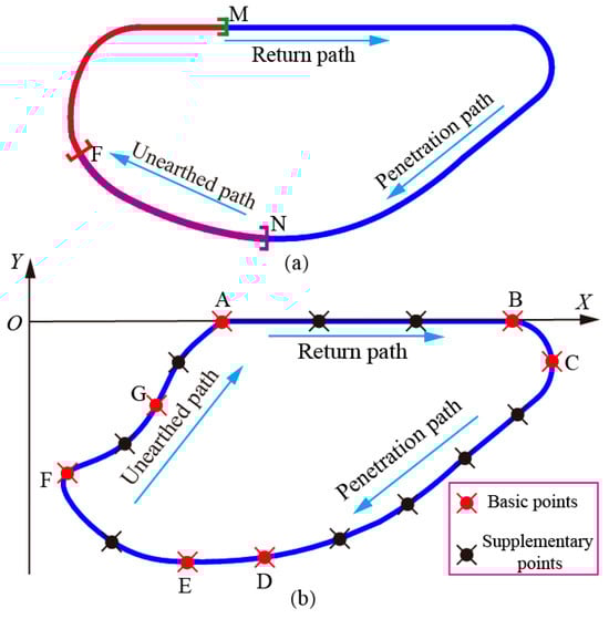
Figure 1. (a) The original bionic subsoiling trajectory, (b) The optimized ideal subsoiling trajectory.

The original bionic subsoiling trajectory is shown in Figure 1a. The N-F-M segment is the unearthed trajectory, where the N-F segment corresponds to the disturbance stage of the subsoiler in the middle and deep soil layers. The curvature radius of this trajectory is increased to allow it to disturb the middle and deep soil layers more extensively. The F-M segment corresponds to the stage where the subsoiler disturbs the shallow soil. It can be concluded that the subsoiler will significantly lift the shallow soil due to the convex shape of this trajectory, causing a large range of disturbance to the shallow soil, leading to excessive moisture loss through evaporation [19]. Based on the principle that the motion trajectory of a tillage tool directly governs its soil disturbance behavior [20], the F-M segment is improved to an inner concave shape to immediately evacuate the shallow soil after the subsoiler disturbs the middle and deep soil, avoid causing extensive overturning of the shallow soil. The optimized improved subsoiling trajectory is shown in Figure 1b. A rectangular coordinate system was established on this trajectory, A, B, C, D, E, F, G are basic type value points, and nine supplementary type value points were evenly inserted into the basic type value points to more accurately discretize the trajectory. The coordinates of 16 points are shown in Table 1 and are defined as improved target trajectory points. The subsoiling mechanism that reproduces the improved trajectory has the potential to improve the soil disturbance effect, increase the damaging range of the plough pan, and reduce tillage resistance.

Table 1. Coordinates of Ideal Target Trajectory Points.

No.	1	2	3	4	5	6	7	8
Pxd	594	642	602	542	476	398	312	223
Pyd	0	−45	−105	−154	−206	−244	−266	−271
No.	9	10	11	12	13	14	15	16
Pxd	135	85	141	184	214	262	374	486
Pyd	−247	−171	−143	−95	−45	0	0	0

2.2. Path Synthesis for the Stephenson III Six-Bar Subsoiling Mechanism

For the path synthesis of complex trajectories, without prescribed timing, with super multiple value points, the six-bar mechanism has the advantages of high accuracy and large solution domain, which is conducive to quickly searching for solutions with high accuracy under additional constraints. In addition, the six-bar mechanism has stable structure and strong load-bearing capacity and is suitable for high-load conditions such as subsoiling. The kinematic chain of the six-bar mechanism can be topologically divided into the Watt type and Stephenson type. Watt I, Stephenson I, and Stephenson II each contain two three-rod linkages, which is not conducive to the lightweight design of the subsoiling mechanism. Because of the existence of three pairs of side links in Watt II, the solution domain of the complex trajectory can be reduced, and the output dyad (actuator rod and second rocker) of the Stephenson III mechanism establishes a direct and dedicated load path to the frame, effectively separating the motion-generation function from the force-bearing function, so the Stephenson type III six-bar mechanism was chosen to reproduce the improved subsoiling trajectory.

2.2.1. Establishment of the Position Function

The Stephenson III six-bar mechanism is composed of a group of Grashof four-bar mechanisms and a group of 2R kinematic chains. The frame and the four-bar mechanism’s coupler link have evolved into three rods. The schematic diagram of the predetermined six-bar subsoiling mechanism is shown in Figure 2, where $r_1$, $r_2$, $r_3$, $r_4$, $r_5$, $r_6$, $r_7$, respectively, represent the lengths of the first frame AD, crank AB, coupler link BC, first rocker CD, actuator rod EF, second rocker FG, and second frame AG. ${\theta }_0$ is the angle between the first frame and the X-axis. ${\theta }_1$ is the angle between the first frame and the second frame. ${\theta }_2$ is the angle between the crank and the first frame, which is defined as the input angle. $\gamma$ is the angle between the coupler link and the first frame. $\psi$ is the angle between the coupler link and the horizontal direction. $\alpha$ is the angle between the actuator rod and the horizontal direction. $\zeta$ is the angle between the second rocker and line GE. $\eta$ is the angle between line GE and the X-axis counterclockwise direction. p₁ and q₁ are vectors for determining the position of point E on the coupler link, while p₂ and q₂ are vectors for determining the position of point P on the actuator rod. The P point on the execution rod is the expected point to achieve the desired subsoiling trajectory.

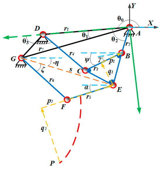
Figure 2. The schematic diagram of the predetermined six-bar subsoiling mechanism.

The position functions of point B and point D are expressed by Equations (1) and (2):

$$\begin{array}{l}{x}_B=x_A+r_2\cdot \cos ({\theta }_2+{\theta }_0)\\ y_B=y_A+r_2\cdot \sin ({\theta }_2+{\theta }_0)\end{array}$$

(1)

$$\begin{array}{l}{x}_D=x_A+r_1\cdot \cos {\theta }_0\\ y_D=y_A+r_1\cdot \sin {\theta }_0\end{array}$$

(2)

The closed-loop vector equation of the Grashof four-bar mechanism ABCD is expressed by Equation (3):

$$r_2{e}^{i{\theta }_2}+r_3{e}^{i\gamma }=r_4{e}^{i{\theta }_3}+r_1$$

(3)

According to Euler’s formula in Equation (4):

$$\begin{array}{l}{r}_2\cdot \cos {\theta }_2+r_3\cdot \cos \gamma -r_4\cdot \sin {\theta }_3-r_1=0\\ r_2\cdot \sin {\theta }_2+r_3\cdot \sin \gamma -r_4\cdot \sin {\theta }_3=0\end{array}$$

(4)

Solving the equation system yields:

$$\gamma =2\arctan ({\displaystyle \frac{K_2^{\prime }-\sqrt{K_1^{\prime 2}+K_2^{\prime 2}-K_3^{\prime 2}}}{K_1^{\prime }-K_3^{\prime }}})$$

(5)

where

$$\begin{array}{l}{K}_1^{\prime }=2a^{\prime }{r}_3,K_2^{\prime }=2b^{\prime }{r}_3,K_3^{\prime }={a^{\prime }}^2+{b^{\prime }}^2+r_3^2-r_4^2\\ a^{\prime }=r_2\cos {\theta }_2-r_1\\ b^{\prime }=r_2\sin {\theta }_2\end{array}$$

(6)

From this, the position of point E can be determined as shown in Equation (7):

$$\begin{array}{l}{x}_E=x_B+p_1\cdot \cos \psi +q_1\cdot \cos ({\displaystyle \frac{\pi }{2}}+\psi )\\ y_E=y_B+p_1\cdot \sin \psi +q_1\cdot \sin ({\displaystyle \frac{\pi }{2}}+\psi )\end{array}$$

(7)

where

$$\psi =\arctan ({\displaystyle \frac{y_B-y_C}{y_B-y_C}})$$

(8)

$$\begin{array}{l}{x}_C=x_B+r_3\cdot \cos ({\theta }_0+\gamma )\\ y_C=y_B+r_3\cdot \sin ({\theta }_0+\gamma )\end{array}$$

(9)

The distance s between point E and point G is expressed by Equation (10):

$$s=\sqrt{{(y_E-y_A-y_{DA}-y_{GD})}^2+{(x_E-x_A-x_{DA}-x_{GD})}^2}$$

(10)

where

$$\begin{array}{l}{x}_{DA}=x_D-x_A\\ y_{DA}=y_D-y_A\\ x_{GD}=x_G-x_D\\ y_{GD}=y_G-y_D\end{array}$$

(11)

$$\begin{array}{l}{x}_G=x_A+r_7\cdot \cos ({\theta }_0+{\theta }_1)\\ y_G=y_A+r_7\cdot \sin ({\theta }_0+{\theta }_1)\end{array}$$

(12)

From this, the position of point F can be determined as shown in Equation (13):

$$\begin{array}{l}{x}_F=x_A+x_{DA}+x_{GD}+r_6\cdot \cos (\eta -\zeta )\\ y_F=y_A+y_{DA}+y_{GD}+r_6\cdot \sin (\eta -\zeta )\end{array}$$

(13)

where

$$\zeta =\arccos ({\displaystyle \frac{r_6^2+s^2-r_5^2}{2s{r}_6}})$$

(14)

$$\eta =\arctan ({\displaystyle \frac{y_E-y_A-y_{DA}-y_{GD}}{x_E-x_A-x_{DA}-x_{GD}}})$$

(15)

Finally, the position function of point P can be obtained as shown in Equation (16):

$$\begin{array}{l}{x}_P=x_E+p_2\cdot \cos \alpha +q_1\cdot \cos ({\displaystyle \frac{\pi }{2}}+\alpha )\\ y_P=y_E+p_2\cdot \sin \alpha +q_2\cdot \sin ({\displaystyle \frac{\pi }{2}}+\alpha )\end{array}$$

(16)

where

$$\alpha =\arctan ({\displaystyle \frac{y_F-y_E}{x_F-x_E}})$$

(17)

2.2.2. Establishment and Solution of the Optimization Model

To pass through 16 ideal target trajectory points in sequence, the objective function is to minimize the position error in the form of the sum of the squares of the Euclidean distances between the ideal target trajectory points $(P_{xd}^i,P_{yd}^i)$ and the corresponding time order P points $(x_p^i,y_p^i)$ as shown in Equation (18):

$$f_{obj}={\displaystyle \sum _{i=1}^{16}\left[{\left(P_{xd}^i-x_p^i(X)\right)}^2+{\left(P_{yd}^i-y_p^i(X)\right)}^2\right]}$$

(18)

The vector X composed of design variables is expressed by Equation (19):

$$X=\left[r_1,r_2,r_3,r_4,r_5,r_6,r_7,p_1,q_1,p_2,q_2,{\theta }_0,{\theta }_1,x_0,y_0,{\theta }_2^1,{\theta }_2^2,\dots {\theta }_2^{16}\right]$$

(19)

The constraint conditions are:

(a)

The Grashof condition for ensuring full rotation of the crank:

$$\left[Max(r_1,r_2,r_3,r_4)+Min(r_1,r_2,r_3,r_4)\right]\le \left\{Sum(r_1,r_2,r_3,r_4)-\left[Max(r_1,r_2,r_3,r_4)+Min(r_1,r_2,r_3,r_4)\right]\right\}$$

(b)

The order conditions for increasing or decreasing the input angle ${\theta }_2$ in order:

$$\begin{array}{l}if{\theta }_2^j=Min\{{\theta }_2^i\},{\theta }_2^j<{\theta }_2^{\mathrm{mod}(j+1,N)}<\dots <{\theta }_2^{\mathrm{mod}(j+N,N)},\\ if{\theta }_2^j=Max\{{\theta }_2^i\},{\theta }_2^j>{\theta }_2^{\mathrm{mod}(j+1,N)}>\dots >{\theta }_2^{\mathrm{mod}(j+N,N)}\end{array}$$

(c)

The assembly conditions for the second rocker and the actuator rod:

$$\begin{array}{l}Max(s)\le r_5+r_6\\ Min(s)\ge \left|r_5-r_6\right|\end{array}$$

(d)

The range of parameters to be solved:

${\theta }_0$ is limited to intervals $\left(\pi ,{\displaystyle \frac{3\pi }{2}}\right)$ and every rod length to intervals $\left(0,500\right)$, and other parameters are continuously adjusted and selected within a reasonable range.

Add conditions (a), (b), and (c) as penalty functions to the objective function, and establish an optimization model as shown in Equation (20):

$$Min\left\{{\displaystyle \sum _{i=1}^{16}\left[{\left(P_{xd}^i-x_p^i(X)\right)}^2+{\left(P_{yd}^i-y_p^i(X)\right)}^2\right]}+\mathrm{M}{h}_1(X)+\mathrm{M}{h}_2(X)+\mathrm{M}{h}_3(X)\right\}$$

(20)

where $h_1(X)$ is taken as 0 when the condition (a) is met, otherwise it is taken as 1. $h_2(X)$ is taken as 0 when the condition (b) is met, otherwise it is taken as 1. $h_3(X)$ is taken as 0 when the condition (c) is met, otherwise it is taken as 1. M is the penalty coefficient, taken as 100.

2.3. EDEM Simulation Model and Simulation Parameters

For the six-bar subsoiling mechanism synthesized in Section 2.2.2, the P point is used as the position of the subsoiler tip, and combined with the optimized process parameter group in Section 3.2.3, a bionic six-bar subsoiling mechanism (B-6-S-M) that can reproduce the ideal subsoiling trajectory was designed, and ADAMS-EDEM coupling simulation was conducted for subsoiling (Figure 3). Compare it with the bionic 4-bar subsoiling mechanism (B-4-S-M) designed by our research team to reproduce the excavation trajectory of moles under the same conditions. Observing the tillage process, it can be seen that the two types of subsoiling mechanisms were in the soil penetration stage from 0 to 0.12 s, in the unearthed stage from 0.12 to 0.32 s, and in the return stage from 0.32 to 0.4 s.

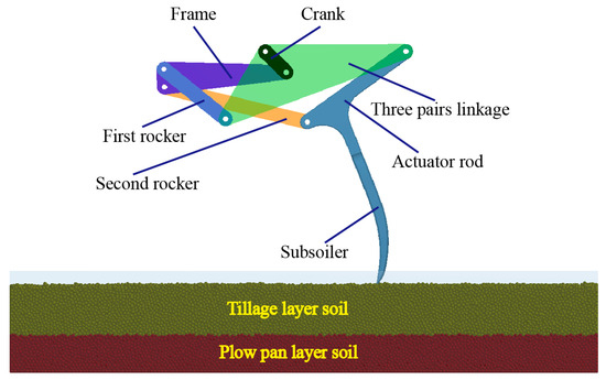
Figure 3. Discrete Element Simulation Model for B-6-S-M.

The EDEM simulation parameters refer to our team’s prior calibration results [6]. The specific material and contact parameters are summarized in Table 2. In [6], these parameters were rigorously calibrated through a series of experiments, including angle-of-repose tests for the cultivated layer and shear tests for the plough pan layer. The cultivated layer parameters were obtained from the angle-of-repose tests, whereas the plough pan was modeled using a bonding contact model, with cohesion and shear strength determined from the shear tests. The calibration process also included a Plackett–Burman experimental design for sensitivity screening, followed by Box–Behnken experiments to further optimize the key parameters.

Table 2. The required parameters in EDEM.

Parameter Type Check	Parameter Name	Value
Material parameter	Soil particle radius (mm)	6
	soil particle density (g/cm3)	1.85
	Poisson’s ratio of soil particles	0.38
	Shear modulus of soil (Pa)	1 × 106
	Subsoiling shovel material density—65 Mn (kg/m3)	7800
	Poisson’s ratio of subsoiler material	0.3
	Shear modulus of subsoiler material (Pa)	7 × 109
Contact parameters	Coefficient of restitution for soil–soil	0.202
	Coefficient of soil–soil friction	0.326
	Coefficient of soil–soil rolling friction	0.02
	Coefficient of restitution for soil—65 Mn	0.35
	Coefficient of soil—65 Mn static friction	0.85
	Coefficient of soil—65 Mn rolling friction	0.1
	Soil JKR surface energy (J/m3)	5.03
	Normal stiffness per unit area (N/m3)	6,892,525
	Tangential stiffness per unit area (N/m3)	7,151,484
	Critical normal stress (Pa)	4,995,000
	Critical tangential stress (Pa)	751,133
	Bond radius (mm)	6.5

2.4. Evaluation Indicators for Tillage Performance

Average tillage resistance is one of the important indicators for evaluating tillage performance [21]. Subsoiling requires breaking the plough pan and significantly disturbing the middle and deep layers of soil to promote the transport of water and nutrients to crop roots. Meanwhile, excessive disturbance of shallow soil will accelerate water evaporation, which is not conducive to water resource protection and crop absorption of water [22]. Therefore, a reasonable soil disturbance effect should cause greater disturbance to the middle and deep layers of soil and minimize disturbance to the shallow layers of soil as much as possible. In addition, the more soil is discharged, the greater the improvement of soil internal porosity. Under the premise of a good soil disturbance effect, the greater the amount of soil that is discharged, the better the tillage performance [23]. Based on our previous research on establishing the discrete element soil model, after the simulation of subsoiling, detection domains were established in the middle and deep layers of soil, shallow soil layer, and areas outside the surface. The number of broken bonds can reflect the breaking ability of the subsoiling mechanism in the plough pan, and the number of soil particles outside the surface can reflect the dumping capacity. The number of soil particles that generate velocity can represent soil disturbance. The disturbance effect is evaluated by the ratio of the disturbance amount t in the middle and deep layers of soil to the disturbance amount s in the shallow layers of soil as shown in Equation (21):

$$k={\displaystyle \frac{t}{s}}$$

(21)

where $k$ is the disturbance coefficient, and the soil disturbance coefficient reflects the ratio of effective soil loosening volume to the total disturbed soil volume. A higher value indicates more efficient subsoiling performance, which is desirable for achieving better root growth conditions and soil structure improvement.

3. Results and Discussion

3.1. Optimization of Six-Bar Subsoiling Mechanism and Process Parameters Based on IDE

Optimization Model Solution

To rigorously evaluate the performance of the optimization model established in Section 2, the Improved Differential Evolution (IDE) algorithm was employed to resolve the six-bar deep-loosening mechanism, and the resultant optimized dimensional parameters are summarized in Table 3. Figure 4a is a schematic diagram of the solution mechanism, with ADG as the three-pair frame rod, AB as the crank, BCE as the three-pair coupler link, CD as the first rocker, GF as the second rocker, and EF as the actuator rod. The iteration curve of the objective function is shown in Figure 4b. When the iteration reaches 8000~10,000 times, the objective function converges to 438, with a solution error of 0.007. The comparison between the ideal target trajectory points and the occurrence trajectory is shown in Figure 4c. All target trajectory points are accurately distributed on the occurrence trajectory.

Table 3. The dimensional parameters of the solution mechanism (length unit: mm; angle unit: rad).

$r_1$	$r_2$	$r_3$	$r_4$	$r_5$	$r_6$	$r_7$	$x_0$
415.97	100.27	266.18	269.29	412.64	498.25	417.21	331.13
$y_0$	$p_1$	$q_1$	$p_2$	$q_2$	${\theta }_0$	${\theta }_1$	${\theta }_2^1$
705.62	243.67	−411.23	−547.18	−588.89	3.1152	0.1480	5.1987
${\theta }_2^2$	${\theta }_2^3$	${\theta }_2^4$	${\theta }_2^5$	${\theta }_2^6$	${\theta }_2^7$	${\theta }_2^8$	${\theta }_2^9$
5.7731	6.1343	0.1044	0.3413	0.5824	0.8514	1.1793	1.6287
${\theta }_2^{10}$	${\theta }_2^{11}$	${\theta }_2^{12}$	${\theta }_2^{13}$	${\theta }_2^{14}$	${\theta }_2^{15}$	${\theta }_2^{16}$	Error
2.5113	3.1323	3.4827	3.7350	4.0528	4.4073	4.7596	0.007

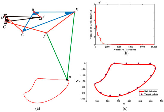
Figure 4. IDE solution results. (a) Schematic diagram of the synthesized six-bar mechanism and its coupler curve, (b) typical response, (c) comparison between the trajectory of point P on the coupler link.

Nominal dimensions are listed to two decimal places for clear presentation, but conventional processing/assembly tolerances are inevitable. This study adopts ISO 2768-1 general tolerances (±0.1–0.2 mm) [24], H7/h6 fits for rotating pairs, and bushings/needle bearings and achieves an assembly accuracy of ±0.2° through fixture alignment.

3.2. Box–Behnken Experimental Results and Process Parameter Optimization

3.2.1. Results of the Box–Behnken Test

The penetration angle is defined as the angle between the subsoiler and the ground when cutting into the soil. It determines the posture of the subsoiler and affects the tillage effectiveness. The study by Hang et al. [21] showed that the distance between shovel teeth has a significant impact on soil disturbance. In addition, the input speed and forward speed of tillage tools also have a significant impact on tillage resistance and soil disturbance performance. The tillage performance is evaluated by four indicators: average tillage resistance, the number of broken bonds in the plough pan, disturbance coefficient, and the number of soil particles outside the surface. Taking the four process parameters of the six-bar subsoiling mechanism, namely the penetration angle (A), distance between shovel teeth (B), forward speed (C), and input speed (D), as experimental factors, and using the average tillage resistance ($f_1$), the number of broken bonds in plough pan ($f_2$), soil disturbance coefficient ($f_3$), and soil discharge amount ($f_4$) as response indicators, a Box–Behnken experiment with four factors and three levels was designed to optimize the working parameters of the subsoiling mechanism. The experimental scheme and results are shown in Table 4. The range of experimental factors is determined by single-factor experiments.

Table 4. Box–Behnken design.

Number	A (°)	B (mm)	C (m/s)	D (r/min)	${\mathit{f}}_1$ (N)	${\mathit{f}}_2$	${\mathit{f}}_3$	${\mathit{f}}_4$
1	97.50	222.50	0.20	150.00	315.04	16,151	1.03	8994
2	120.00	185.00	0.35	120.00	291.37	15,647	1.09	5888
3	97.50	222.50	0.35	120.00	251.07	14,413	0.92	5198
4	75.00	222.50	0.35	150.00	310.81	15,633	0.95	8148
5	75.00	260.00	0.35	120.00	277.74	14,481	0.86	4718
6	97.50	222.50	0.20	90.00	221.71	14,203	0.88	3572
7	97.50	185.00	0.35	150.00	310.76	15,721	1.15	9852
8	97.50	185.00	0.20	120.00	270.94	15,634	1.04	6335
9	75.00	222.50	0.20	120.00	341.1	15,282	0.92	7694
10	97.50	260.00	0.20	120.00	261.89	15,227	0.87	5622
11	120.00	222.50	0.35	90.00	239.63	13,793	0.93	2870
12	75.00	222.50	0.35	90.00	238.66	13,033	0.92	2450
13	120.00	222.50	0.35	150.00	354.15	16,132	1.12	9112
14	97.50	260.00	0.35	90.00	219.00	13,590	0.87	2917
15	97.50	260.00	0.35	150.00	289.1	14,716	0.92	7325
16	97.50	185.00	0.50	120.00	248.38	13,863	1.04	4634
17	97.50	222.50	0.50	150.00	290.62	15,120	0.97	7696
18	75.00	222.50	0.50	120.00	271.11	13,577	0.96	4061
19	97.50	222.50	0.50	90.00	207.42	12,312	0.92	2487
20	97.50	185.00	0.35	90.00	220.46	13,648	1.00	3136
21	97.50	222.50	0.35	120.00	251.12	14,433	0.93	5186
22	120.00	260.00	0.35	120.00	273.77	14,647	0.93	5081
23	97.50	260.00	0.50	120.00	240.14	13,501	0.9	4207
24	97.50	222.50	0.35	120.00	251.23	14,435	0.93	5164
25	75.00	185.00	0.35	120.00	279.22	15,168	1.07	5119
26	97.50	222.50	0.35	120.00	251.54	14,410	0.94	5187
27	120.00	222.50	0.20	120.00	293.44	16,011	1.00	6101
28	120.00	222.50	0.50	120.00	279.24	14,063	0.97	4890
29	97.50	222.50	0.35	120.00	251.59	14,422	0.92	5183

3.2.2. Regression Model Evaluation and Experimental Results Analysis

Design-Expert 13 software was used to analyze experimental data and fit the data using quadratic polynomial functions to obtain regression models between various response indicators and experimental factors.

(a)

Regression model for average tillage resistance is shown in Equation (22):

$$\begin{array}{l}{f}_1=4.20e^{-3}{D}^2+299.39C^2-3.88e^{-4}{B}^2+6.50e^{-2}{A}^2-0.56CD\\ -4.89e^{-3}BD+3.60e^{-2}BC+1.57e^{-2}AD+4.13AC-4.78e^{-3}AB\\ +0.11D-645.87C+1.03B-14.89A+909.79\end{array}$$

(22)

The $R^2$ and $R_{adj}^2$ values are 0.9548 and 0.9095, respectively, indicating that the regression model has good predictive ability for experimental data. The variance analysis of the average tillage resistance regression model is shown in Table 5. The overall p value of the model is less than 0.0001, indicating that the regression model is highly significant. From the p value of each factor, it can be determined that C and D have a significant impact on the average tillage resistance. The degree of influence of the four influencing factors on the average tillage resistance is D, C, B, and A in descending order [25].

Table 5. Variance analysis of the average tillage resistance.

Source	Sum of Squares	DF	Mean Square	F Value	p Value
Model	34,264.03	14	2447.43	21.10	<0.0001
A	14.00	1	14.00	0.12	0.7334
B	294.92	1	294.92	2.54	0.1331
C	2329.93	1	2329.93	20.09	0.0005
D	22,846.41	1	22,846.41	197.00	<0.0001
AB	64.96	1	64.96	0.56	0.4666
AC	778.13	1	778.13	6.71	0.0214
AD	448.80	1	448.80	3.87	0.0693
BC	0.16	1	0.16	1.414 × 10−3	0.9705
BD	102.01	1	102.01	0.88	0.3642
CD	25.65	1	25.65	0.22	0.6454
A2	7015.70	1	7015.70	60.50	<0.0001
B2	1.94	1	1.94	0.017	0.8990
C2	294.34	1	294.34	2.54	0.1335
D2	92.56	1	92.56	0.80	0.3868
Residual	1623.56	14	115.97
Lack of fit	1623.33	10	162.33	2806.11	<0.0001
Pure error	0.23	4	0.058

(b)

Regression model for the number of broken bonds in the plough pan is shown in Equation (23):

$$\begin{array}{l}{f}_2=-9.56e^{-2}{D}^2+1125.56C^2+9.79e^{-2}{B}^2+0.67A^2+47.78CD\\ -0.21BD+2.00BC-9.67e^{-2}AD-18.00AC-9.27e^{-2}AB\\ +98.32D-\mathrm{10,806.78}C-17.80B-81.15A+\mathrm{15,487.42}\end{array}$$

(23)

The $R^2$ and $R_{adj}^2$ values are 0.9701 and 0.9402, respectively, indicating that the regression model has good predictive ability for experimental data. From Table 6, it can be seen that the regression model shows a highly significant level, with B, C, and D having a significant impact on the number of broken bonds in the plough pan.

Table 6. Variance analysis of the number of broken bonds in the plough pan.

Source	Sum of Squares	DF	Mean Square	F Value	p Value
Model	2.559 × 107	14	1.828 × 106	32.43	<0.0001
A	8.107 × 105	1	8.107 × 105	14.38	0.0020
B	1.032 × 106	1	1.032 × 106	18.31	0.0008
C	8.454 × 106	1	8.454 × 106	149.97	<0.0001
D	1.385 × 107	1	1.385 × 107	245.79	<0.0001
AB	24,492.25	1	24,492.25	0.43	0.5205
AC	14,762.25	1	14,762.25	0.26	0.6168
AD	17,030.25	1	17,030.25	0.30	0.5912
BC	506.25	1	506.25	8.981 × 10−3	0.9258
BD	2.242 × 105	1	2.242 × 105	3.98	0.0660
CD	1.849 × 105	1	1.849 × 105	3.28	0.0916
A2	7.529 × 105	1	7.529 × 105	13.36	0.0026
B2	1.230 × 105	1	1.230 × 105	2.18	0.1618
C2	4160.14	1	4160.14	0.074	0.7898
D2	48,169.50	1	48,169.50	0.85	0.3709
Residual	7.892 × 105	14	56,368.59
Lack of fit	7.886 × 105	10	78,864.71	614.69	<0.0001
Pure error	513.20	4	128.30

(c)

Regression model for the disturbance coefficient is shown in Equation (24):

$$\begin{array}{l}{f}_3=2.47e^{-5}{D}^2+0.10C^2+2.29e^{-5}{B}^2+5.88e^{-5}{A}^2-5.56e^{-3}CD\\ -2.22e^{-5}BD+1.33e^{-3}BC+5.93e^{-5}AD-5.19e^{-3}AC+1.48e^{-5}AB\\ -3.10e^{-3}D+0.82C-1.18e^{-2}B-1.87e^{-2}A+3.28\end{array}$$

(24)

The $R^2$ and $R_{adj}^2$ values are 0.9837 and 0.9674, respectively, indicating that the regression model has good predictive ability for experimental data. According to Table 7, the regression model shows a highly significant level, with A, B, D, AD, A², and B² having a significant impact on the disturbance coefficient.

Table 7. Variance analysis of the soil disturbance coefficients.

Source	Sum of Squares	DF	Mean Square	F Value	p Value
Model	0.16	14	0.011	60.32	<0.0001
A	0.011	1	0.011	57.49	<0.0001
B	0.090	1	0.090	479.80	<0.0001
C	3.333 × 10−5	1	3.33 × 10−5	0.18	0.6800
D	0.032	1	0.032	170.52	<0.0001
AB	6.250 × 10−4	1	6.250 × 10−4	3.33	0.0896
AC	1.225 × 10−3	1	1.225 × 10−3	6.52	0.0230
AD	6.400 × 10−3	1	6.400 × 10−3	34.07	<0.0001
BC	2.250 × 10−4	1	2.250 × 10−4	1.20	0.2923
BD	2.500 ×10−3	1	2.500 × 10−3	13.31	0.0026
CD	2.500 × 10−3	1	2.500 × 10−3	13.31	0.0026
A2	5.741 × 10−3	1	5.741 × 10−3	30.56	<0.0001
B2	6.746 × 10−3	1	6.746 × 10−3	35.91	<0.0001
C2	3.284 × 10−5	1	3.284 × 10−5	0.17	0.6822
D2	3.211 × 10−3	1	3.211 × 10−3	17.09	0.0010
Residual	2.630 × 10−3	14	1.879 × 10−4
Lack of fit	2.350 × 10−3	10	2.350 × 10−4	3.36	0.1272
Pure error	2.800 × 10−4	4	7.000 × 10−5

(d)

Regression model for soil discharge amount is shown in Equation (25):

$$\begin{array}{l}{f}_4=0.49D^2+6975.56C^2-1.81e^{-2}{B}^2+0.27A^2-11.83CD\\ -0.51BD+12.71BC+0.20AD+179.41AC-0.12AB\\ +74.83D-\mathrm{29,529.44}C+65.55B-106.42A+89.69\end{array}$$

(25)

The $R^2$ and $R_{adj}^2$ values are 0.9766 and 0.9531, respectively, indicating that the regression model has good predictive ability for experimental data. From Table 8, it can be seen that the regression model reaches a highly significant level, and the impact of C and D on the soil discharge amount is extremely significant.

Table 8. Variance analysis of the soil discharge amount.

Source	Sum of Squares	DF	Mean Square	F Value	p Value
Model	1.103 × 108	14	7.879 × 106	41.69	<0.0001
A	2.558 × 105	1	2.558 × 105	1.35	0.2641
B	2.162 × 106	1	2.162 × 106	11.44	0.0045
C	8.915 × 106	1	8.915 × 106	47.17	<0.0001
D	9.461 × 107	1	9.461 × 107	500.59	<0.0001
AB	41,209.00	1	41,209.00	0.22	0.6477
AC	1.467 × 106	1	1.467 × 106	7.76	0.0146
AD	73,984.00	1	73,984.00	0.39	0.5416
BC	20,449.00	1	20,449.00	0.11	0.7471
BD	1.332 × 106	1	1.332 × 106	7.05	0.0189
CD	11,342.25	1	11,342.25	0.060	0.8100
A2	1.214 × 105	1	1.214 × 105	0.64	0.4362
B2	4193.06	1	4193.06	0.022	0.8837
C2	1.598 × 105	1	1.598 × 105	0.85	0.3734
D2	1.257 × 106	1	1.257 × 106	6.65	0.0219
Residual	2.646 × 106	14	1.890 × 105
Lack of fit	2.645 × 106	10	2.645 × 105	1736.97	<0.0001
Pure error	609.20	4	152.30

Although the lack of fit was significant, the high R² and adjusted R² values (both > 0.9), together with the strong significance of the main factors, indicate that the regression model still possesses excellent predictive capability and is reliable for optimization within the studied factor ranges. (Although the lack of fit term was statistically significant, this is not uncommon in response surface methodology studies, especially when higher-order interactions beyond the quadratic model may exist. Importantly, the regression models in this study still exhibited high coefficients of determination ($R^2$ > 0.95, $R_{adj}^2$ > 0.90), and the main experimental factors (C and D) were highly significant. These results indicate that the models retain strong predictive capability and reliability within the studied factor ranges and thus can be effectively applied for optimization purposes).

3.2.3. Process Parameter Optimization Based on Satisfaction Function Method

The satisfaction function method is a commonly used multiresponse optimization method, whose basic principle is to convert multiple response indicators into a single comprehensive satisfaction through weighting [26]. A regression model comprehensively reflects the four response indicators through a satisfaction function. For the average tillage resistance, it is hoped that the smaller the value, the better, and it is transformed into a smaller satisfaction function. For the other three indicators, the larger the expected value, the better, and it will be converted into a satisfaction function. The upper and lower limits of the four indicators are taken from the single factor test results in Table 3, with each response weight set at 0.25.

The satisfaction function of average tillage resistance is expressed by Equation (26):

$$d_1=\left\{\begin{array}{c}0\hspace{1em}\hspace{1em}\hspace{1em}\hspace{1em} f_1<207.42\\ {\displaystyle \frac{354.15-f_1}{354.15-207.42}}\hspace{1em}207.42\le f_1\le 354.15\\ 1\hspace{1em}\hspace{1em}\hspace{1em}\hspace{1em} f_1>354.15\end{array}\right.$$

(26)

The satisfaction function of the number of broken bonds is expressed by Equation (27):

$$d_2=\left\{\begin{array}{c}\hfill 0\hspace{1em}\hspace{1em}\hspace{1em}\hspace{1em} f_2<\mathrm{12,312}\hfill \\ {\displaystyle \frac{f_2-\mathrm{12,312}}{\mathrm{16,151}-\mathrm{12,312}}}\hspace{1em}\mathrm{12,312}\le f_2\le \mathrm{16,151}\\ \hfill 1\hspace{1em}\hspace{1em}\hspace{1em}\hspace{1em} f_2>\mathrm{16,151}\hfill \end{array}\right.$$

(27)

The satisfaction function of soil disturbance coefficient is expressed by Equation (28):

$$d_3=\left\{\begin{array}{c}\hfill 0\hspace{1em}\hspace{1em}\hspace{1em}\hspace{1em}{f}_3<0.86\hfill \\ {\displaystyle \frac{f_3-0.86}{1.15-0.86}}\hspace{1em}0.86\le f_3\le 1.15\\ \hfill 1\hspace{1em}\hspace{1em}\hspace{1em}\hspace{1em}{f}_3>1.15\hfill \end{array}\right.$$

(28)

The satisfaction function of soil discharge amount is expressed by Equation (29):

$$d_4=\left\{\begin{array}{c}\hfill 0\hspace{1em}\hspace{1em}\hspace{1em}\hspace{1em}{f}_4<2450\hfill \\ {\displaystyle \frac{f_4-2450}{9852-2450}}\hspace{1em}2450\le f_4\le 9852\\ \hfill 1\hspace{1em}\hspace{1em}\hspace{1em}\hspace{1em}{f}_4>9852\hfill \end{array}\right.$$

(29)

The overall comprehensive satisfaction function is expressed by Equation (30):

$$Q= (d_1\cdot d_2\cdot d_3\cdot d_4{)}^{0.25}$$

(30)

An optimization model for the satisfaction function can be established as shown in Equation (31):

$$Max[({\displaystyle \frac{354.15-f_1}{354.15-207.42}}\times {\displaystyle \frac{f_2-\mathrm{12,312}}{\mathrm{16,151}-\mathrm{12,312}}}\times {\displaystyle \frac{f_3-0.86}{1.15-0.86}}\times {\displaystyle \frac{f_4-2450}{9852-2450}}){]}^{0.25}$$

$$\mathrm{s}.\mathrm{t}.\left\{\begin{array}{c}75\le A\le 120\\ 185\le B\le 260\\ 0.2\le C\le 0.5\\ 90\le D\le 150\end{array}\right.$$

(31)

The optimization model was solved using the genetic algorithm. Figure 5 shows the iteration curve of the satisfaction function. After about 100 iterations, the satisfaction function value converged to the optimal solution, corresponding to the optimal combination of process parameters: A is 99.61°, B is 185 mm, C is 0.29 m/s, and D is $5\mathrm{\pi }$ rad/s. The predicted values of the corresponding response indicators under the optimal solution are: $f_1$ is 305.36 N, $f_2$ is 16,352, $f_3$ is 1.16, and $f_4$ is 9922. Using the optimal parameter combination for discrete element simulation of the six-bar subsoiling mechanism, the value of the response index was obtained as follows: average tillage resistance was 316.12 N, and the relative error of the predicted value was 3.40%. The number of broken bonds in the plough pan is 15,591, with a relative error of 4.88%. The soil disturbance coefficient is 1.26, with a relative error of 7.93%. The soil discharge amount is 10,326, with a relative error of 3.91%, which verifies the reliability of the optimization model and the accuracy of the optimal process parameter group.

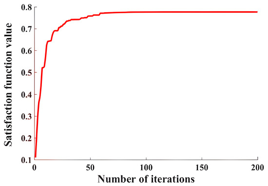
Figure 5. The iteration curve of the satisfaction function.

3.3. Comparison of Tillage Performance

3.3.1. Tillage Resistance

Figure 6 shows the curve of tillage resistance with time for B-4-S-M and B-6-S-M. During the soil penetration stage, due to the same subsoiling trajectory of the two mechanisms, there is not much difference in resistance. During the unearthed stage, B-6-S-M experienced significantly less tillage resistance than B-4-S-M due to the implementation of the concave improved F-A trajectory. The average tillage resistance of B-4-S-M and B-6-S-M were 350.89 N and 316.12 N, respectively, and the average resistance decreased from 350.89 N to 316.12 N, a reduction of 9.91%. As shown in Figure 7, the visualization cloud diagram of the subsoiler’s resistance under the driving of two mechanisms at 0.13 s and 0.20 s was used to represent the stress situation during the soil penetration and un-earthed stages. The color represents the size, and the red area on the surface of the subsoiler driven by B-6-S-M is significantly less than that of B-4-S-M, which intuitively indicates that B-6-S-M has resistance reduction performance.

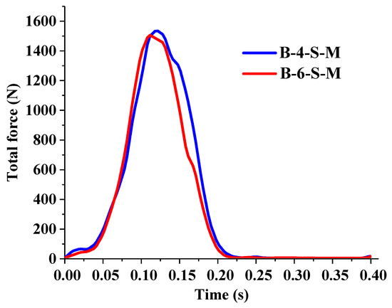
Figure 6. Variation curve of tillage resistance.

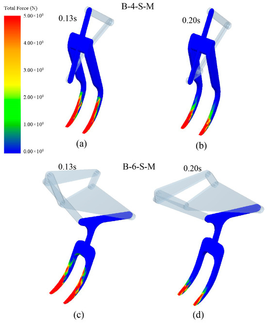
Figure 7. The visualization cloud diagram of the subsoiler’s resistance: (a,b) B-4-S-M, (c,d) B-6-S-M.

3.3.2. Soil Disturbance Performance

In Figure 8, the curves of the number of broken bonds in the plough pan over time under the action of the two subsoiling mechanisms are shown. The numbers of broken bonds by B-4-S-M and B-6-S-M are 14,958 and 15,591, respectively, indicating that the destructive ability of B-6-S-M on the plough pan soil has increased by 4.23%. Figure 9 shows a visualization of the broken bonds by the subsoiler. B-6-S-M acts on the plough pan for a longer time, resulting in a greater range and intensity of damage to the plough pan.

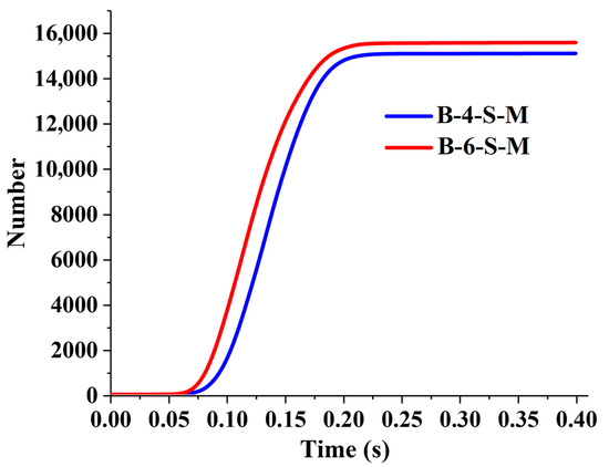
Figure 8. The curve of the number of broken bonds in the plough pan.

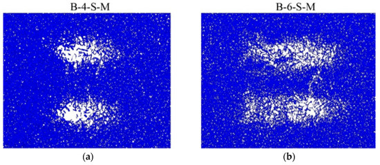
Figure 9. Visualization of the broken bonds by (a) B-4-S-M, (b) B-6-S-M.

Figure 10 shows a visualized cloud diagram of particle velocity under the action of the two subsoiling mechanisms during the unearthed stage, with colors representing size. Due to the optimization of the trajectory during the unearthed stage, B-6-S-M causes significantly less disturbance to the topsoil layer than B-4-S-M. Figure 11 and Figure 12 show the particle number curves (soil disturbance curves) for the production speed of middle-depth and shallow soil layers, respectively. The disturbance of B-6-S-M to the middle and deep soil is always greater than that of B-4-S-M. During the interaction between the two subsoiling mechanisms and the shallow soil, the disturbance of B-6-S-M to the shallow soil is significantly smaller than that of B-4-S-M. Under the action of B-4-S-M and B-6-S-M, the numbers of particles that generated velocity in shallow soil were 6481 and 5888, respectively, and the numbers of particles that generated velocity in deep soil were 6217 and 8044, respectively. B-6-S-M reduced the disturbance to shallow soil by 14.43%, increased the disturbance to deep soil by 29.54%, and the disturbance coefficients of B-4-S-M and B-6-S-M were 0.96 and 1.37, respectively, improving the disturbance effect by 42.71%.

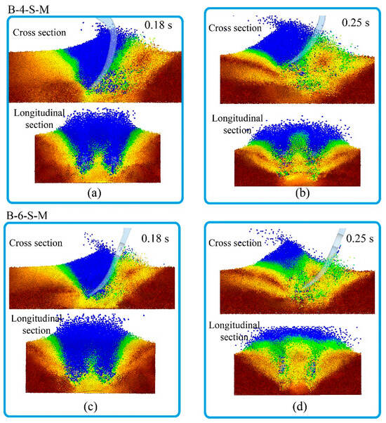
Figure 10. Visualized cloud diagram of particle velocity during the unearthed stage for (a,b) B-4-S-M, (c,d) B-6-S-M.

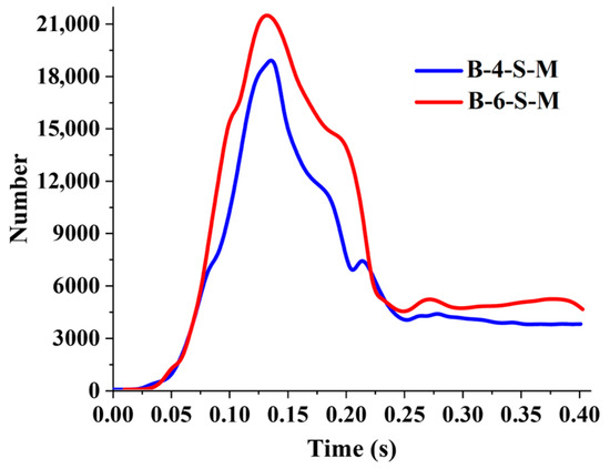
Figure 11. Soil disturbance curves of middle-depth soil layer.

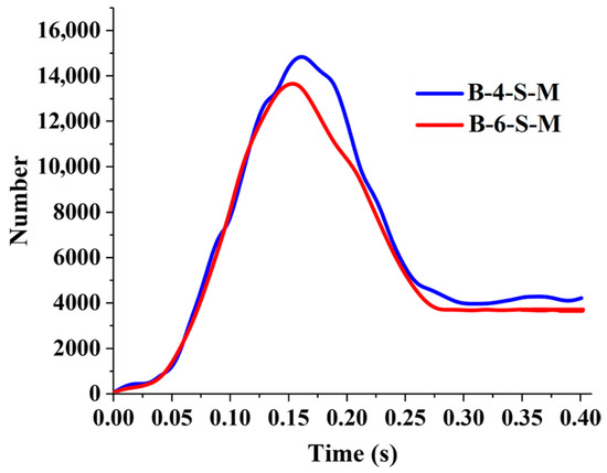
Figure 12. Soil disturbance curves of shallow soil layer.

The curves of the discharge amount of the two subsoiling mechanisms are shown in Figure 13. During the period of 0.05 to 0.2 s, the subsoiler disturbed the middle and deep layers of soil, and the soil discharge of B-6-S-M was greater than that of B-4-S-M, indicating that B-6-S-M had a greater disturbance amplitude on the plough pan and could better improve the porosity of the middle and deep soil layers. In the following time period, B-6-S-M caused less disturbance to shallow soil, so the soil discharged amount was less than that of B-4-S-M.

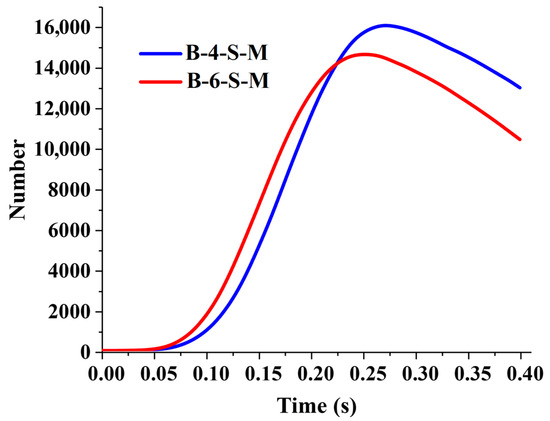
Figure 13. The variation curves of the discharge amount.

3.4. Finite Element Analysis of Subsoiler

In order to better restore the stress and strain generated in the process of subsoiler tillage, the force data of the subsoiler when it breaks into the bottom of the plough pan (0.08 s), shovels into the bottom of the plough pan (0.12 s), and leaves the plough pan (0.18 s) were imported from EDEM 2020 to the ANSYS 2020R2 Workbench Statics module for coupling analysis. Figure 14 shows the force data export interface in EDEM, and Figure 15 shows the coupling interface of the force data export between Workbench and EDEM.

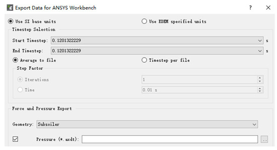
Figure 14. Export of force data in EDEM.

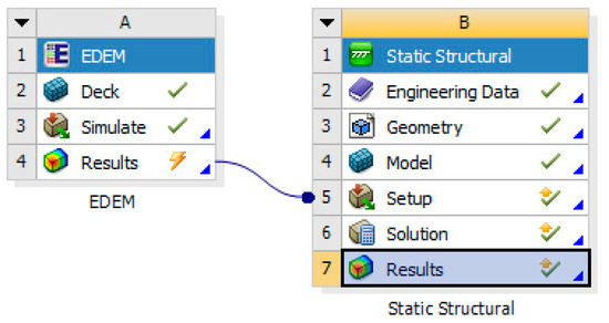
Figure 15. EDEM–Workbench coupling module.

Figure 16 shows the total deformation and equivalent stress cloud map of the subsoiler at three times. The maximum deformation part of the subsoiler is at the shovel tip, and the deformation gradually decreases from the shovel tip to the shovel handle. The total deformation when breaking into the plough pan is 3.4915 mm, when digging into the bottom layer, the total deformation is 2.5533 mm, when leaving the plough pan, the maximum deformation is 3.1572 mm, and when digging into the bottom layer, the total deformation is the maximum, and the maximum deformation is less than 0.1 mm, meeting the design requirements of 65 Mn material for the subsoiler. The stress of the subsoiler gradually decreases and diffuses outward from the handle and tooth root, with the maximum stress at the connection between the execution rod and the shovel handle. The maximum stresses at three times are 11.548 Mpa, 21.752 Mpa, and 17.453 Mpa, respectively. When the shovel enters the bottom, the stress is the highest, and the maximum stress is far less than the yield strength of 65 Mn, proving that the subsoiler can meet the strength requirements.

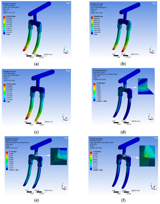
Figure 16. Total Deformation and Equivalent Stress Contour Plots of the Subsoiler Shovel: (a–c) Subsoiler’s deformation cloud map when breaking into the plough pan, digging into the bottom layer, and leaving the plough pan, (d–f) Subsoiler’s equivalent force cloud diagram when breaking into the plough pan, digging into the bottom layer, and leaving the plough pan.

3.5. Experiment

3.5.1. Prototype Processing and Assembly

With reference to the assembled six-bar subsoiling mechanism model prototype in Solidworks, an indoor soil bin test was conducted (Figure 17). In accordance with the design scheme of the discrete element soil model, the length, width, and height of the indoor soil bin were set to 100 cm, 60 cm, and 35 cm, respectively. Appropriate amounts of cultivated layer soil and plough pan soil were excavated from the test field. During the filling of the soil bin, 15 cm thick plough pan soil was first added and squeezed down to 12 cm thick with a wooden board to simulate the compact and hard characteristics of the plough pan soil, and then 18 cm thick cultivated layer soil was placed into the soil bin.

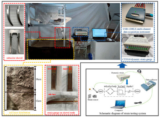
Figure 17. Soil bin test.

A worm gear reduction motor with a power of 1.5 kW (Hangzhou Saili Reduction Equipment Factory, Hangzhou, China), a reduction ratio of 1:15, and a torque of 132 Nm was selected as the driving motor. During operation, the subsoiler shovel must penetrate the ground surface and fragment the hard, compact plough pan. Should the strength of the shovel teeth be insufficient, deformation or fracture is highly probable. Consequently, the material chosen for manufacturing the subsoiler shovel must possess both adequate strength and good wear resistance. Manganese steel, which exhibits high strength and excellent wear resistance, is well-suited to harsh operating conditions involving impact, compression, and abrasion. For this reason, 65 Mn steel (Jiaxing Lankalan Intelligent Equipment Co., Ltd., Pinghu City, China) was selected for fabricating the teeth of the bionic subsoiler shovel, as illustrated in Figure 17. A pair of shovel teeth are fixedly attached to the shovel handle via bolts.

Dynamic changes in the tillage resistance of the subsoiler shovel were collected using strain gauges and a testing system. The testing system consists of hardware and software components. The hardware includes 120–100 AA strain gauges (with a resistance of 120 Ω and a sensitivity of 2) (Ningzhou Yinzhou Xiaying Chenyue Mechanical & Electrical Equipment Business Department, Ningbo, China), a CT5310 dynamic strain gauge (equipped with 10 channels), and a USB-1208LS multichannel data acquisition instrument (Shanghai Chengke Electronics Co., Ltd., Shanghai, China). The software component is the DAQmni 4.1 data processing software.

The bridge connection scheme is shown in Figure 18, using a half-bridge single-compensation form, with the workpiece connected to the AB bridge. A strain gauge is attached to the block with the same material but without stress, and it is put together with the test piece so that it is in the same temperature field. As a temperature-compensation piece, it is connected to the BC bridge, and other bridge arms are linked inside the instrument.

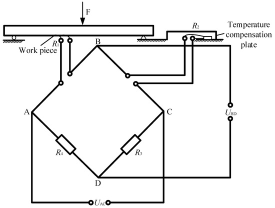
Figure 18. Bridge connection scheme of strain gauge.

To reduce the errors caused by instrument manufacturing accuracy and experimental operations, the parameters that determine the strain load relationship are calibrated. The linear relationship between strain and load F can be expressed as Equation (32):

$$\mathrm{\Delta }\epsilon =aF+b$$

(32)

where a and b are calibration coefficients.

As shown in Figure 19, the test piece is loaded and unloaded using a hydraulic universal testing machine, and the load and strain values are read during the steady phase. Ten tests are performed on each group of adhesive positions, and one set of calibration coefficient values is obtained every two tests. The average of five sets of coefficients is taken as the final calibration coefficient for each group of adhesive positions, as shown in Table 9. The strain data can be converted into load data through Equation (33), and the working resistance curve can be plotted.

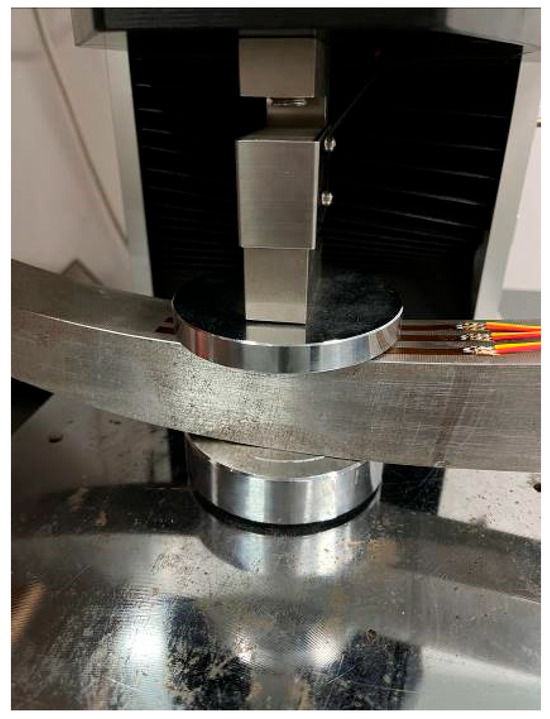
Figure 19. Hydraulic universal testing machine.

Table 9. Calibration results.

Coefficient	Upper End of Soil Contact Surface	Lower End of Soil Contact Surface
a	0.65	0.62
b	3.86	2.53

As shown in Figure 17, three strain gauge are pasted on the upper and lower ends of the subsoiler contact surface, and one strain gauge is pasted on both sides. In the process of pasting, the pasting part was polished, rust removed, marked, and positioned, the part surface was wiped off with acetone cotton, the strain gauge lead was welded to the terminal, the adhesive (502 glue) was evenly applied on the bottom of the strain gauge to paste the train gauge at the appropriate position, and some terminals were pasted.

The signal wires on the strain gauges are connected to the dynamic strain gauge, which consists of a Wheatstone bridge, a filter, and an amplifier. It can amplify the tiny voltage signals output by the bridge before transmitting them. Finally, the signals are displayed on a computer with data processing software installed via the data acquisition instrument. During the operation of the subsoiling mechanism, data is collected using DAQmni software. The output voltage variation curves are observed, and the data is exported. The strain data is converted using the following Formula (33):

$$\mathrm{\Delta }\epsilon ={\displaystyle \frac{4\times (U_1-U_0)\times {10}^6}{k_1\times U_2\times n\times Ks}}$$

(33)

where $\mathrm{\Delta }\epsilon$ is the strain value, $U_1$ and $U_0$ are the load output voltage and no-load output voltage, respectively (unit: V), $k_1$ is the sensitivity coefficient of the strain gauge, $U_2$ and Ks are the bridge pressure and instrument gain coefficient, respectively (both are given when the instrument leaves the factory), and n is the number of useful bridge arms.

Based on the principle of the strain testing system and the mapping relationship between the output voltage of the bridge and the load, the resistances acting on the upper end, lower end, and both side faces of the soil-contacting surface of the subsoiler shovel during tillage were measured respectively. The actual tillage resistance of the subsoiler shovel can be obtained by summing up the resistances on these three contact surfaces.

The evaluation scheme for soil disturbance is as follows: after laying the plough pan soil in the soil bin, a subsoiling operation is carried out to observe the appearance and morphology of the plough pan soil after being broken, which are then compared with the visual images from the simulation results. The soil disturbed by the subsoiler shovel during the soil emergence stage is retained, and the disturbance and soil discharge status of each soil layer are observed on the corresponding cross-sections, which are further compared with the visual images from the simulation results.

3.5.2. Experimental Result Analysis

Under the conditions of the optimal process parameter group, DEM simulations of subsoiling and indoor soil bin subsoiling tests were conducted respectively, with a comparative analysis performed on the subsoiling effects.

Figure 20 shows a comparison between the prototype test and simulation process of a six-bar subsoiling mechanism at three different times. The mechanism cuts into the soil, lifts the soil, and causes appropriate disturbance. When leaving the soil, some soil is excluded from the surface, and the simulation and experimental subsoiling process are basically consistent.

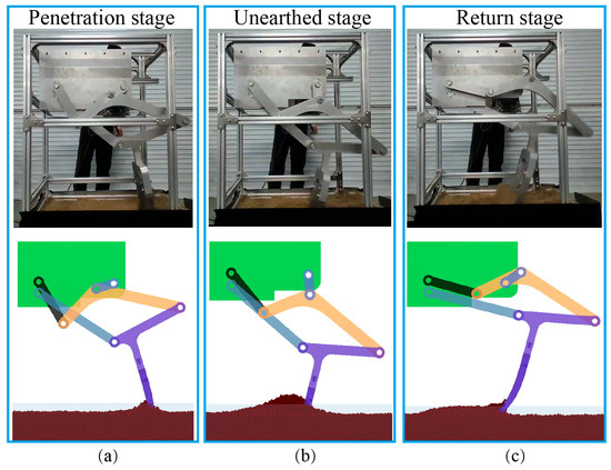
Figure 20. Soil disturbance process (a) Penetration stage, (b) Unearthed stage, and (c) Return stage.

Figure 21 shows a comparison of the total tillage resistance curves between the experiment and simulation. The variation patterns of the two curves are consistent with the analysis in Section 3.1. Due to the difficulty of measuring the concentrated stress generated at the tip of the subsoiler using the adhesive strain measurement method, the measured tillage resistance is generally slightly lower than the simulation value. During the penetration stage, the stress concentration at the shovel tip is relatively high, and the deviation is relatively large. The unearthed stage mainly involves the force on the front shovel surface with a small deviation. During the return stage, the shovel tip is subjected to resistance from the surface soil, resulting in a certain deviation. The simulated and measured values of tillage resistance at each sampling point have average levels of 281.32 N and 258.83 N, respectively, with a relative error of 8.67%. This indicates that the model established in this study can accurately simulate the actual tillage resistance of subsoiling.

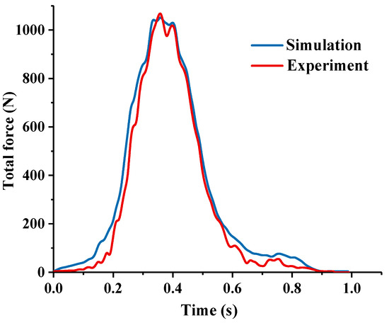
Figure 21. Tillage resistance variation curve in experiments and simulations.

Figure 22 shows the comparison between the test results and the simulation results of the damage to the plough bottom after deep loosening. The range and depth of the damage to the plough bottom caused by the deep loosening shovel in the test are basically consistent with the simulation results.

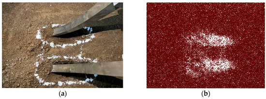
Figure 22. Plough pan breakage condition: (a) Experiment, (b) Simulation.

Figure 23 shows the comparison of the test results and simulation results of the soil disturbance situation. The disturbance range and soil discharge conditions of each soil layer in the test are basically consistent with the simulation results and conform to the analysis in Section 3.2, verifying that the discrete element simulation can accurately simulate the soil disturbance behavior of deep loosening shovels.

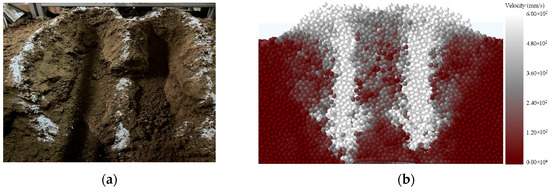
Figure 23. The Soil layer disturbance and discharge condition: (a) Experiment, (b) Simulation.

Limitations: Due to equipment constraints, the soil box test was performed as a single verification run without replicates or error bars. The goal here is model–experiment agreement under a representative condition; comprehensive statistical inference across soil types is deferred to future work, where replicated tests with error bars on clay and loam soils will be conducted.

4. Conclusions

Based on the agricultural needs and our research on a bionic four-bar subsoiling mechanism, an improved bionic subsoiling trajectory was given, A new six-bar subsoiling mechanism of the Stephenson III type that can reproduce the trajectory is proposed, and its structure parameters are optimized, combined with an improved difference algorithm. Its optimal process parameters are obtained using the satisfaction function method. Combining the discrete element method, the tillage performances of the four-bar subsoiling mechanism and the six-bar subsoiling mechanism were compared. The finite element analysis of the subsoiler was conducted using the EDEM Workbench coupling simulation method, and indoor soil box experiments were conducted on the physical prototype. The following conclusions can be drawn:

(1)

When the improved differential algorithm was used to solve the path generation optimization model, the objective function converges to 438 when iterated to 80,000~10,000 times, with a solution error of 0.007. All target trajectory points were accurately distributed on the occurring trajectory. It is proved that the improved differential algorithm can accurately solve the Stephenson III type six-bar mechanism that can reproduce the improved subsoiling trajectory.

(2)

The satisfaction function method was used to convert multiple response indicators into a single comprehensive satisfaction function. The satisfaction function was optimized and the optimal process parameter combination of the six-bar subsoiling mechanism was obtained: the penetration angle was 99.61°, the shovel distance was 185 mm, the forward speed was 0.29 ms⁻¹, and the input speed was $5\pi$ rad/s.

(3)

Under the optimal combination of process parameters, the tillage performances of the four-bar subsoiling mechanism and the six-bar subsoiling mechanism were com-pared using the discrete element method. The results showed that the resistance reduction rate of the six-bar subsoiling mechanism was 9.91%, the damage ability to the plough pan was increased by 4.23%, the disturbance to the shallow soil was reduced by 14.43%, the disturbance to the middle and deep soil was increased by 29.54%, and the disturbance effect was improved by 42.71%, which proved the significance of combining agronomy to optimize bionic trajectory.

(4)

Simulations and subsoiling tests on a six-bar subsoiling mechanism were conducted, combined with a strain testing system to obtain data on changes in tillage resistance of the subsoiler, observing and analyzing the soil disturbance process. The results showed that the simulated and measured values of average tillage resistance were 281.32 N and 258.83 N, respectively, with a relative error of 8.67%. The damage range and depth of the subsoiler in the plough pan, the disturbance range of each soil layer, and the soil discharge status in the experiment were basically consistent with the simulation results.

It is verified that the method and model in this study can accurately represent the soil behavior of the subsoiler. The prototype of the six-bar subsoiling mechanism can achieve significant reduction in resistance and a high-efficiency soil loosening effect.

References

- Zhang, X.N.; You, Y.; Wang, D.C.; Wang, Z.Y.; Liao, Y.Y.; Li, S.B. Soil failure characteristics and loosening effectivity of compacted grassland by subsoilers with different plough points. Biosyst. Eng. 2023, 237, 170–181. [Google Scholar] [CrossRef]
- Gao, Z.C.; Song, B.Q.; Gao, Z.C.; Song, B.Q.; Wang, C.L.; Gao, W.C.; Zhang, L.L.; Sun, L.; Hao, X.Y.; Liu, F. Soil amelioration by deep ploughing of different machineries and its effect on promoting crop growth and yield. Trans. Chin. Soc. Agric. Eng. 2018, 34, 79–86. [Google Scholar] [CrossRef]
- Xue, S.P.; Wu, M.F.; Jia, Z.K.; Zhu, L. Small Single Shovel Subsoiling Machine. CN Patent Application No. 201042118Y, 2 April 2008. [Google Scholar]
- Hu, W.W.; Nie, H.L.; Chen, X.F.; Liu, M.J.; Qi, J.B.; Ding, J.X. Experimental Study on Crawler Type Narrow Width Mini Deep Loosening Machine. Agric. Eng. 2020, 10, 14–17. [Google Scholar] [CrossRef]
- Zhang, L.; Zhai, Y.B.; Wu, C.Y.; Huang, S.Z.; Zhang, Z.E. Modeling the Interaction between a New Four-Bar Subsoiling Mechanism and Red Soil Using the Improved Differential Evolution Algorithm and DEM. Comput. Electron. Agric. 2023, 208, 107783. [Google Scholar] [CrossRef]
- Zhang, L.; Zhai, Y.B.; Chen, J.N.; Zhang, Z.E.; Huang, S.Z. Optimization Design and Performance Study of a Subsoiler Underlying the Tea Garden Subsoiling Mechanism Based on Bionics and EDEM. Soil Tillage Res. 2022, 220, 105375. [Google Scholar] [CrossRef]
- Acharyya, S.K.; Mandal, M. Performance of EAs for Four-Bar Linkage Synthesis. Mech. Mach. Theory 2009, 44, 1784–1794. [Google Scholar] [CrossRef]
- Peñuñuri, F.; Peón-Escalante, R.; Villanueva, C.; Pech-Oy, D. Synthesis of Mechanisms for Single and Hybrid Tasks Using Differential Evolution. Mech. Mach. Theory 2011, 46, 1335–1349. [Google Scholar] [CrossRef]
- Cabrera, J.A.; Simon, A.; Prado, M. Optimal Synthesis of Mechanisms with Genetic Algorithms. Mech. Mach. Theory 2002, 37, 1165–1177. [Google Scholar] [CrossRef]
- Bulatović, R.R.; Đorðević, S.R. Optimal Synthesis of a Path Generator Six-Bar Linkage. J. Mech. Sci. Technol. 2012, 26, 4027–4040. [Google Scholar] [CrossRef]
- Shiakolas, P.S.; Koladiya, D.; Kebrle, J. On the Optimum Synthesis of Six-Bar Linkages Using Differential Evolution and the Geometric Centroid of Precision Positions Technique. Mech. Mach. Theory 2005, 40, 319–335. [Google Scholar] [CrossRef]
- Ucgul, M.; Fielke, J.M.; Saunders, C. Three-dimensional discrete element modelling (DEM) of tillage: Accounting for soil cohesion and adhesion. Biosyst. Eng. 2015, 129, 298–306. [Google Scholar] [CrossRef]
- Wang, Y.M.; Xue, W.L.; Ma, Y.H.; Tong, J.; Liu, X.P.; Sun, J.Y. DEM and soil bin study on a biomimetic disc furrow opener. Comput. Electron. Agric. 2019, 156, 209–216. [Google Scholar] [CrossRef]
- Zeng, Z.W.; Ma, X.; Chen, Y.; Qi, L. Modelling Residue Incorporation of Selected Chisel Ploughing Tools Using the Discrete Element Method (DEM). Soil Tillage Res. 2020, 197, 104505. [Google Scholar] [CrossRef]
- Shaikh, S.A.; Li, Y.M.; Ma, Z.; Chandio, F.A.; Tunio, M.H.; Liang, Z.W.; Solangi, K.A. Discrete Element Method (DEM) Simulation of Single Grouser Shoe-Soil Interaction at Varied Moisture Contents. Comput. Electron. Agric. 2021, 191, 106538. [Google Scholar] [CrossRef]
- Hoseinian, S.H.; Hemmat, A.; Esehaghbeygi, A.; Shahgoli, G.; Baghbanan, A. Development of a Dual Sideway-Share Subsurface Tillage Implement: Part 1. Modeling Tool Interaction with Soil Using DEM. Soil Tillage Res. 2021, 215, 105201. [Google Scholar] [CrossRef]
- Tang, Z.Y.; Gong, H.; Wu, S.L.; Zeng, Z.W.; Wang, Z.Q.; Zhou, Y.H.; Fu, D.B.; Liu, C.; Cai, Y.H.; Qi, L. Modelling of Paddy Soil Using the CFD-DEM Coupling Method. Soil Tillage Res. 2023, 226, 105591. [Google Scholar] [CrossRef]
- Maraveas, C.; Tsigkas, N.; Bartzanas, T. Agricultural Processes Simulation Using Discrete Element Method: A Review. Comput. Electron. Agric. 2025, 237, 110733. [Google Scholar] [CrossRef]
- Kassam, A.; Friedrich, T.; Derpsch, R.; Kienzle, J. Overview of the Worldwide Spread of Conservation Agriculture. Field Actions Sci. Rep. 2015, 8, 1. [Google Scholar]
- Wang, Y.; Zhang, D.; Yang, L.; Cui, T.; Jing, H.; Zhong, X. Modeling the Interaction of Soil and a Vibrating Subsoiler Using the Discrete Element Method. Comput. Electron. Agric. 2020, 174, 105518. [Google Scholar] [CrossRef]
- Li, B.; Chen, Y.; Chen, J. Modeling of Soil–Claw Interaction Using the Discrete Element Method (DEM). Soil Tillage Res. 2016, 158, 177–185. [Google Scholar] [CrossRef]
- Hang, C.G.; Gao, X.J.; Yuan, M.C.; Huang, Y.X.; Zhu, R.X. Discrete Element Simulations and Experiments of Soil Disturbance as Affected by the Tine Spacing of Subsoiler. Biosyst. Eng. 2017, 168, 73–82. [Google Scholar] [CrossRef]
- Sun, J.Y.; Wang, Y.M.; Ma, Y.H.; Tong, J.; Zhang, Z.J. DEM Simulation of Bionic Subsoilers (Tillage Depth >40 cm) with Drag Reduction and Lower Soil Disturbance Characteristics. Adv. Eng. Softw. 2018, 119, 30–37. [Google Scholar] [CrossRef]
- ISO 2768-1:1989; General Tolerances—Part 1: Tolerances for Linear and Angular Dimensions Without Individual Tolerance Indications (ISO System). ISO: Geneva, Switzerland, 1989.
- Ma, W.P.; You, Y.; Wang, D.C.; Yin, S.J.; Huang, X.L. Parameter Calibration of Alfalfa Seed Discrete Element Model Based on RSM and NSGA-II. Trans. Chin. Soc. Agric. Mach. 2020, 51, 136–144. [Google Scholar]
- Li, W.J. Design and Experiment of an Intra-Row Weeding Mechanism Based on Non-Circular Planetary Gear Train. Master’s Thesis, Zhejiang Sci-Tech University, Hangzhou, China, 2022. [Google Scholar]
Disclaimer/Publisher’s Note: The statements, opinions and data contained in all publications are solely those of the individual author(s) and contributor(s) and not of MDPI and/or the editor(s). MDPI and/or the editor(s) disclaim responsibility for any injury to people or property resulting from any ideas, methods, instructions or products referred to in the content. |
© 2025 by the authors. Licensee MDPI, Basel, Switzerland. This article is an open access article distributed under the terms and conditions of the Creative Commons Attribution (CC BY) license (https://creativecommons.org/licenses/by/4.0/).