YOLO-FDLU: A Lightweight Improved YOLO11s-Based Algorithm for Accurate Maize Pest and Disease Detection

Abstract

As a global staple ensuring food security, maize incurs 15–20% annual yield loss from pests/diseases. Conventional manual detection is inefficient (>7.5 h/ha) and subjective, while existing YOLO models suffer from >8% missed detections of small targets (e.g., corn armyworm larva) in complex fields due to feature loss and poor multi-scale fusion. We propose YOLO-FDLU, a YOLO11s-based framework: LAD (Light Attention-Downsampling)-Conv preserves small-target features; C3k2_DDC (DilatedReparam–DilatedReparam–Conv) enhances cross-scale fusion; Detect_FCFQ (Feature-Corner Fusion and Quality Estimation) optimizes bounding box localization; UIoU (Unified-IoU) loss reduces high-IoU regression bias. Evaluated on a 25,419-sample dataset (6 categories, 3 public sources + 1200 compliant web images), it achieves 91.12% Precision, 92.70% mAP@0.5, 78.5% mAP@0.5–0.95, and 20.2 GFLOPs/15.3 MB. It outperforms YOLOv5-s to YOLO12-s, supporting precision maize pest/disease monitoring.

1. Introduction

Maize, a global staple supporting 4.5 billion people’s food security, accounts for ~30% of global cereal production and reached 1.2 billion metric tons in 2024 [1]. However, pests (Ostrinia furnacalis, Spodoptera frugiperda) and diseases (Cercospora zeae-maydis, Puccinia sorghi) cause 15–20% annual yield loss (180–240 million metric tons) and over $30 billion in damages, hitting smallholders the hardest.

Traditional detection relies on manual scouting—inefficient (5–8 hectares/day/inspector), subjective (15–20% misjudgments), and delayed [2]. To address this, deep learning has advanced agricultural detection: Zhang et al. [2] proposed AgriPest-YOLO for pest detection, while Li et al. [3] improved YOLOv8s for corn leaf diseases (mAP@0.5 = 89.4%) but with a bulky 22.6 MB model. YOLO variants (YOLOv5s, YOLOv8s) are widely used for their real-time performance (≥30 FPS on edge devices) [1], yet they struggle in complex fields: de Almeida et al. [4] noted 12–15% false positives from clutter, and Lu et al. [5] highlighted >20% missed detections of small targets (<5 mm) due to poor multi-scale fusion.

To solve these gaps, this study proposes YOLO-FDLU, a YOLO11s-based framework with three core modules (LAD-Conv for small-target features, C3k2_DDC for multi-scale fusion, Detect_FCFQ for false positive reduction). The main contributions of this paper are summarized as follows:

• A modified detection framework based on YOLO11s is proposed for accurate identification of typical maize pests and diseases;
• Multiple lightweight and feature-enhancement modules are constructed and evaluated for their performance improvements;
• A comprehensive evaluation of model precision and robustness is conducted using standard performance metrics and confusion matrices.

Evaluated on 25,419 samples (6 categories), YOLO-FDLU outperforms mainstream YOLOs. This work supports intelligent crop monitoring and precise pest control in agriculture [1,3].

2. Materials and Methods

2.1. Datasets

High-quality pest and disease datasets are fundamental to the reliability of visual detection models. However, existing maize-related datasets often suffer from limitations such as small scale, narrow category coverage, or lack of complex field scenario samples [6,7], which may lead to poor model generalization in real agricultural environments. To address these issues—specifically to enhance the model’s robustness against multiple pest and disease categories under variable field conditions, and to objectively evaluate its performance in detecting both foliar diseases and insect infestations—this study constructed an expanded image dataset combined with diverse data augmentation techniques.

2.1.1. Dataset Description

The dataset used in this study covers six typical maize pest and disease categories, including three foliar diseases and three insect pests: (1) Corn Leaf Blight (CLB), (2) Corn Gray Leaf Spot (CGLS), (3) Corn Rust Leaf (CRL), (4) Corn Armyworm Larva (CAWL), (5) Corn Borer (CB), and (6) Corn Borer Larva (CBL).

The initial image samples (8793 in total) were collected from two sources to ensure diversity and authenticity:

Public datasets: Three well-recognized agricultural datasets were used, including Maize_in_Field_Dataset (containing natural field maize images) [8], IP102 (a large-scale insect pest dataset, with maize pest subsets extracted) [9,10], and Corn or Maize Leaf Disease Dataset (focusing on maize foliar disease images) [11];

Manual collection: Web-sourced images were manually screened to supplement rare samples (e.g., early-stage CAWL), with all collected images verified for copyright compliance and authenticity by agricultural experts.

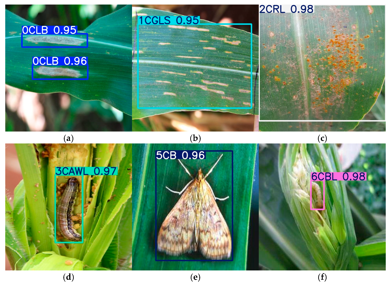
To standardize input for the detection model, all raw images were resized to a fixed resolution of 640 × 640 pixels. Additionally, all samples were annotated using the LabelImg tool (in VOC format) to generate bounding boxes for target regions, and annotations were cross-validated by two plant protection specialists to ensure accuracy. Representative images and their corresponding annotations for each category are presented in Figure 1.

2.1.2. Image Data Augmentation

In practical maize fields, detection models often face interference from variable environmental factors, such as uneven illumination (e.g., direct sunlight, overcast), random camera angles, and leaf occlusion by weeds or adjacent plants. These factors introduce significant noise into image data, and the ability of a deep learning model to perform robust identification under such conditions largely depends on the completeness and diversity of the training dataset [12].

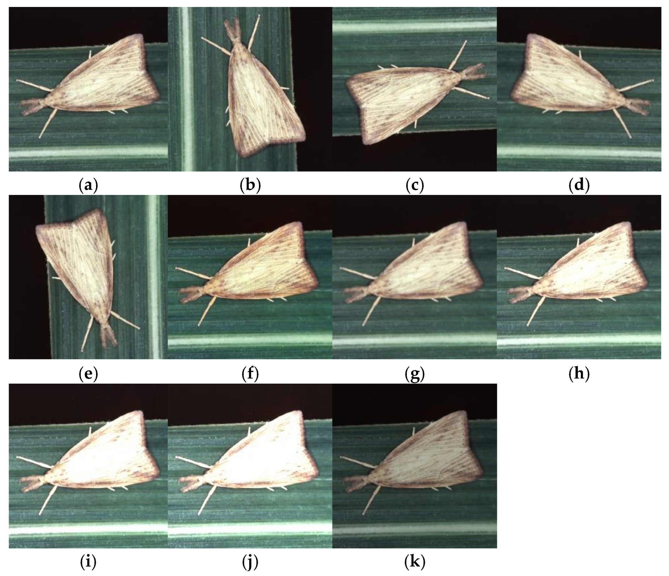
To enhance the model’s generalization capability under diverse field conditions, the original 8793 raw images were augmented using five distinct techniques. These include: (1) image rotation (90°, 180°, and 270°), which has been shown to effectively capture orientation variability in plant disease datasets [13]; (2) horizontal mirroring; (3) color balance adjustment and (4) Gaussian blur (kernel size 3 × 3), both commonly employed to simulate field imaging distortions [14]; and (5) brightness adjustment with multiple scaling factors (0.7, 1.2, 1.4, 1.6), a strategy frequently reported to improve model robustness under varying illumination conditions [15]. Representative examples of these augmentations are shown in Figure 2. This augmentation strategy enriches dataset diversity and helps the model adapt to environmental variability, thereby improving its robustness and stability in real deployment.

2.1.3. Dataset Size Evaluation

After applying the aforementioned augmentation techniques, the initial 8793 images were expanded to 26,376 samples. To balance training quality (sufficient samples for model fitting) and generalization performance (unbiased evaluation of unseen data), the expanded dataset was split into training, validation, and test sets at a ratio of 8:1:1 [16]. This splitting strategy is widely adopted in agricultural computer vision tasks, as it ensures the training set has enough samples to support model learning while the validation/test sets can objectively reflect the model’s practical performance [17,18].

To confirm the rationality of the final dataset size, a preliminary experiment was conducted using the YOLO11s baseline model: training on the 26,376-sample dataset achieved an mAP@0.5 of 90.92%, which exceeds the 90% performance threshold for practical agricultural detection [19]. Further analysis showed that while increasing the dataset size (e.g., to 30,000 samples) could slightly improve detection accuracy (mAP@0.5 increased by 0.3%), it would significantly increase training time (by ~25%) and computational cost (GPU memory usage increased by ~18%), leading to diminishing marginal returns [20]. Therefore, the 26,376-sample dataset was selected as the final training dataset. Detailed variations in detection performance (e.g., Precision and mAP@0.5) across different dataset sizes (8793, 17,598, 26,376 samples) are presented in

Table 1. Comparison of Training Results with Different Dataset Sizes.

Number of Images (pcs)	Precision (%)	mAP@0.5 (%)	Training Time (hours)
8793	76.8	69.5	14.49
17,598	85.8	85.7	28.88
26,376	88.7	90.9	42.34

, which further validates the rationality of this selection.

2.2. YOLO-FDLU Model Design

To address the key challenges of small-target missed detections, insufficient multi-scale feature fusion, and low bounding box localization accuracy of existing YOLO models in complex maize field environments, this study proposes an enhanced detection model based on YOLO11s, named YOLO-FDLU (YOLO with Detect_FCFQ, C3k2_DDC neck, LAD-Conv backbone, and UIoU loss). The following sections detail the structural optimizations and design principles of each core component of YOLO-FDLU.

2.2.1. YOLO-FDLU Architecture

The overall architecture of YOLO-FDLU is illustrated in Figure 3, with the YOLO11s baseline shown above for comparison. YOLO-FDLU retains the lightweight backbone–neck–detection head framework of YOLO11s while introducing four key optimizations to target maize pest and disease detection requirements:

• Backbone optimization: Replacing the standard 3 × 3 stride-2 convolutional downsampling layers at the P3, P4, and P5 stages with the proposed Light Attention-Downsampling Convolution (LAD-Conv) module. This modification addresses the loss of fine-grained features (e.g., early-stage CRL spots, small CAWL) during downsampling, enhancing the model’s ability to capture small-target details;
• Neck optimization: Replacing all original C3k2 modules in the neck (feature fusion stage) with the improved C3k2_DDC (DilatedReparam–DilatedReparam–Conv) module. This strengthens cross-scale feature connectivity (e.g., fusing 2 mm CGLSs and 10 mm CB targets), improving multi-scale detection adaptability;
• Detection head optimization: Replacing the standard Detect module with the custom Detect_FCFQ (Detection Head with Feature-Corner Fusion and Quality Estimation) module. This integrates corner feature fusion and bounding box quality estimation, reducing false positives caused by background clutter (e.g., dry leaves mistaken for CLB);
• Loss function optimization: Integrating the Unified-IoU (UIoU) loss proposed by Luo et al. (2024) [21] to replace the original CIoU loss, enhancing the consistency and accuracy of bounding box regression for irregular targets (e.g., clustered CBL).

Figure 3. Comparison of YOLO11s baseline (top) and YOLO-FDLU model (bottom).

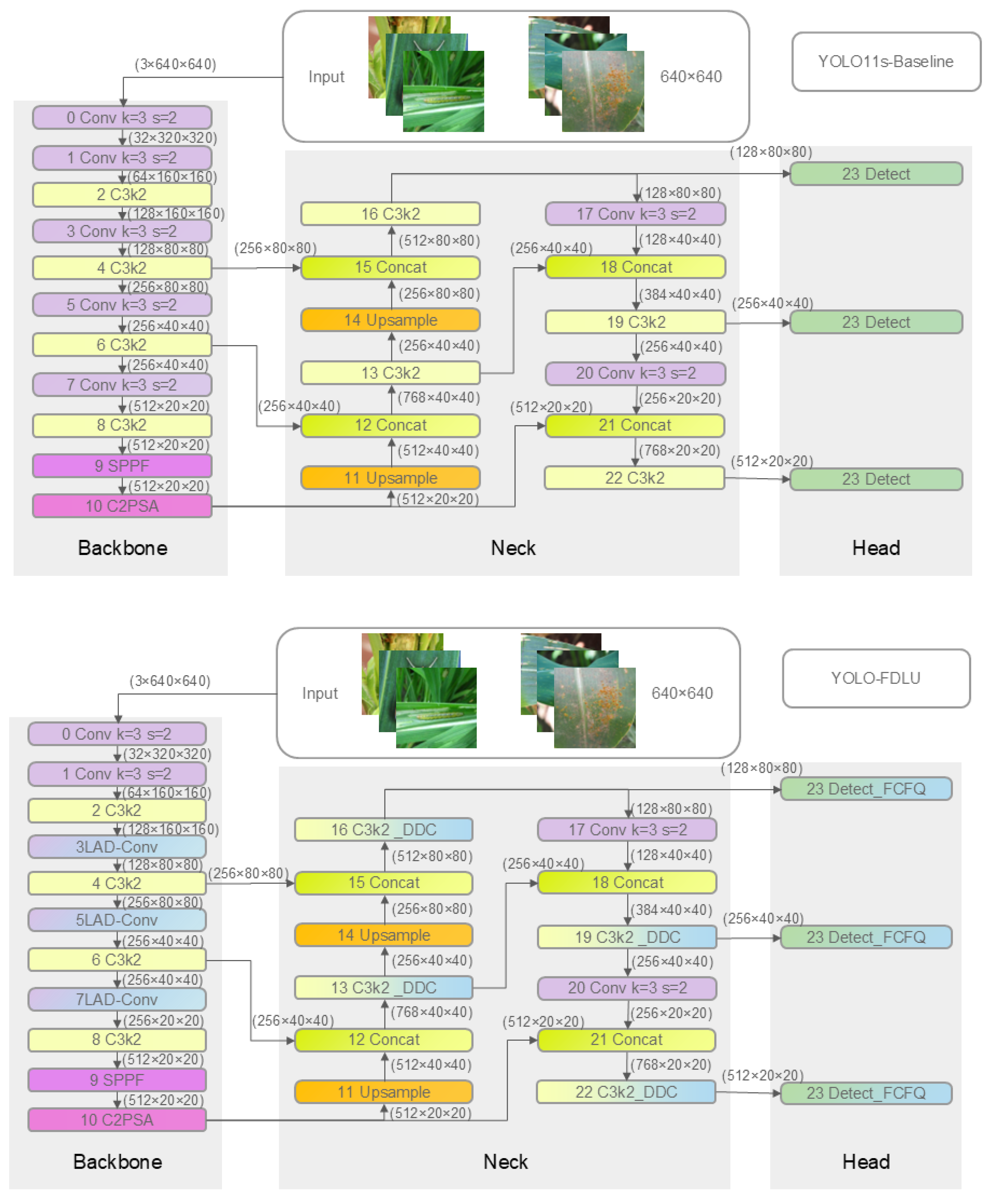
Figure 3. Comparison of YOLO11s baseline (top) and YOLO-FDLU model (bottom).

Additionally, the model retains the SPPF (Spatial Pyramid Pooling—Fast) and C2PSA (Conv2d-PatchEmbed-SelfAttention) modules of YOLO11s to preserve large receptive field perception (critical for detecting widespread foliar diseases like CLB). Deeper C3k2 modules in mid-to-high layers are configured with shortcut = True to strengthen contextual feature aggregation. These optimizations ensure that YOLO-FDLU maintains lightweight characteristics (model size: 15.3 MB, GFLOPs: 20.2) while significantly improving detection performance for maize pests and diseases.

2.2.2. Improved Downsampling Module: LAD-Conv

The LAD-Conv module is designed to address the limitation of conventional downsampling techniques (e.g., stride-2 convolution, max pooling) that discard fine-grained spatial details—details critical for detecting tiny insects (e.g., CAWL, body length < 5 mm) or early-stage leaf lesions (e.g., CGLSs < 2 mm) [22]. It achieves this by introducing a local adaptive weighting mechanism to guide the retention of informative features during downsampling.

• Module Application Scope

Considering computational efficiency and feature importance, LAD-Conv is selectively applied in the YOLO11 backbone to replace downsampling layers at the P3/8, P4/16, and P5/32 stages (corresponding to feature maps with strides of 8, 16, and 32, respectively). Shallow layers (P1/2, P2/4) still adopt standard 3 × 3 stride-2 convolutions, as these layers primarily capture low-level features (e.g., leaf edges) and require rapid spatial compression to avoid excessive computational overhead [23].

2.

Module Structure and Working Principle

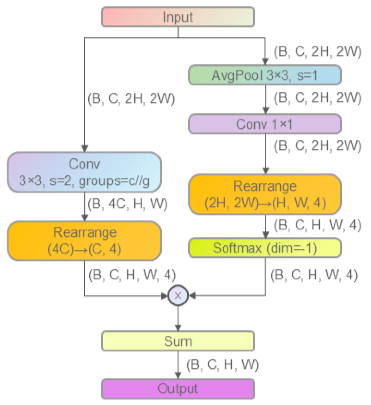
The structure of LAD-Conv is shown in Figure 4, consisting of two parallel branches (attention branch and downsampling convolution branch) that work synergistically to generate the final output:

Attention Branch: First, the input feature map (shape: (B, C, 2H, 2W), where B = batch size, C = number of channels, H = height, W = width) undergoes (3 × 3) average pooling with a stride of 1 to extract local contextual information, resulting in a feature map with shape (B, C, 2H, 2W). Next, a (1 × 1) convolution is applied, keeping the shape as (B, C, 2H, 2W). Then, a rearrangement operation transforms the shape from (2H, 2W) to (H, W, 4), yielding a tensor with shape ((B, C, H, W, 4)). Subsequently, a Softmax activation function (applied along dimension (−1)) is used to generate normalized attention weights for each (2 × 2) local region. The final output of this branch is a weight tensor with shape (B, C, H, W, 4) (the additional “4” dimension corresponds to the four sub-regions in each (2 × 2) block).

Downsampling Convolution Branch: The input feature map is processed via a (3 × 3) grouped convolution with a stride of 2 (number of groups = (C/g)) to compress the spatial dimension (2H × 2W to H × W)) and expand the channel dimension from C to 4C, resulting in an output feature map with shape (B, 4C, H, W). The output feature map is then reshaped via a rearrangement operation from (4C) t (C, 4), obtaining a tensor with shape (B, C, H, W, 4) to align with the attention branch in terms of shape.

Feature Fusion: The outputs of the two branches are fused via element-wise multiplication (weighting the downsampled features with the attention weights), and then a sum operation is performed. The final output feature map has a shape of ((B, C, H, W)). The specific operation is as follows:

$$Y_{b,c,i,j}={\displaystyle \sum _{k=0}^3{\alpha }_{b,c,i,j,k}}\cdot x_{b,c,i,j,k}^{\mathrm{patch}}$$

(1)

where ${\alpha }_{b,c,i,j,k}$: Softmax weights generated by the attention branch.

$x_{b,c,i,j,k}^{\mathrm{patch}}$: Output of the grouped convolution (grouped conv) downsampling branch.

$x\in R^{bs\times ch\times 2H\times 2W}$.

$Y\in R^{bs\times ch\times H\times W}$.

This mechanism adaptively emphasizes the most informative sub-regions within each (2 × 2) block (e.g., CAWL targets in a cluttered background), improving the visibility of small targets in deeper layers—especially under dense, cluttered, or blurry field conditions [24]. By limiting LAD-Conv to the P3–P5 stages, the model maintains low computational overhead while significantly boosting sensitivity to small maize pests and early-stage diseases.

2.2.3. Improved C3k2 Module: C3k2_DDC

The C3k2_DDC module is designed to enhance fine-grained feature recognition in agricultural images—particularly for complex maize pest and disease structures (e.g., irregular CRL pustules, tiny CBL feeding holes)—by improving multi-scale feature fusion in the neck stage. It replaces all original C3k2 modules in the YOLO11 neck to strengthen cross-scale feature connectivity without increasing backbone complexity.

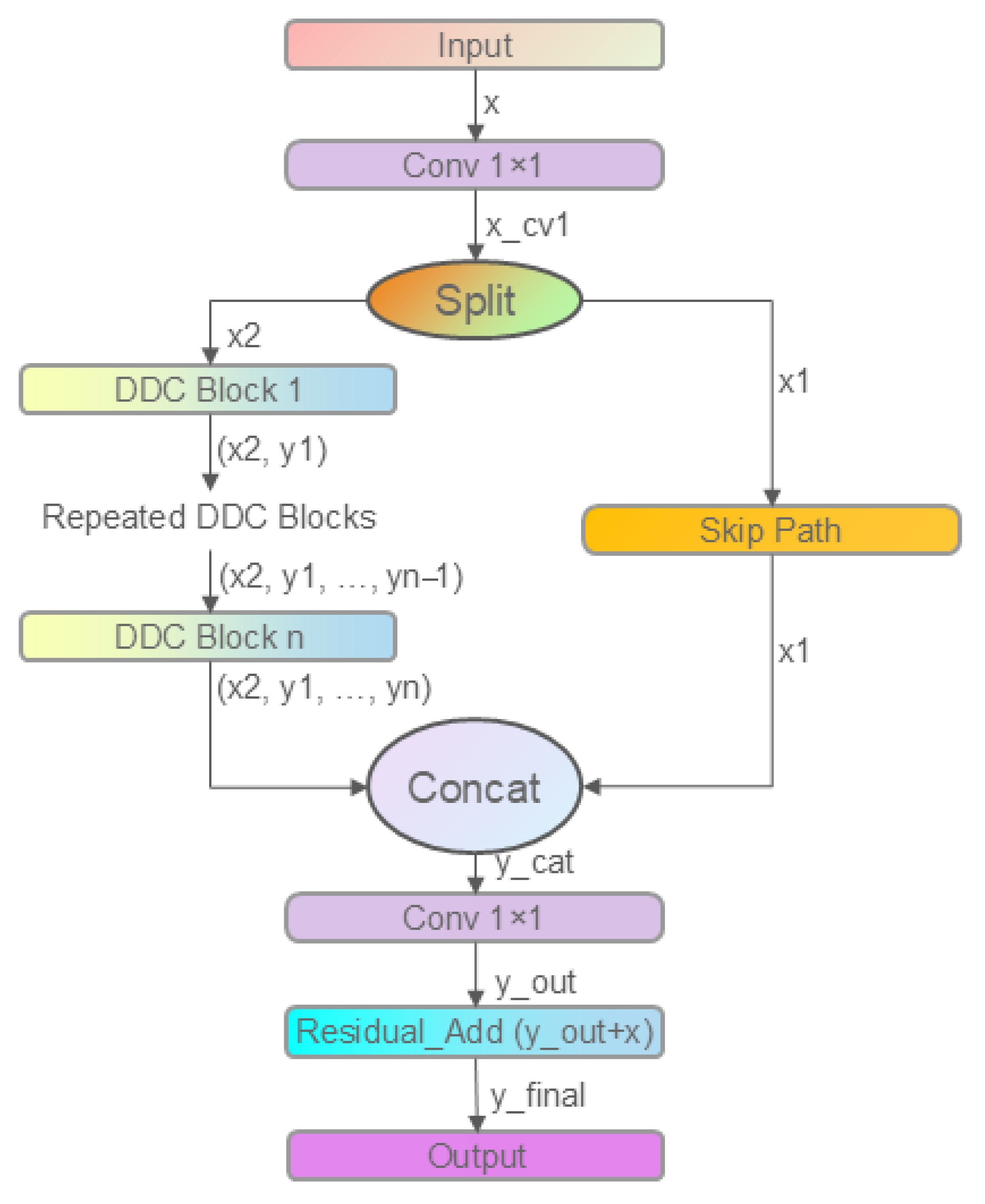
The structure of C3k2_DDC is shown in Figure 5, which inherits the CSP (Cross Stage Partial) architecture and lightweight residual design of the original C3k2 module while introducing the DDC (DilatedReparam–DilatedReparam–Conv) sub-module to enhance multi-scale feature capture (e.g., similar in principle to the grouped dilated convolution module [25] in which demonstrates effective multi-scale feature extraction via dilated convolutions and grouped convolution). The specific workflow is as follows:

The input feature $x$ is first compressed via a 1 × 1 convolution into intermediate feature $x_{cv1}$, then split along the channel dimension into two branches: $x_1$ (residual path) and $x_2$ (transform path).

The $x_2$ branch passes through a series of DDC (DilatedReparam–DilatedReparam–Conv) modules. The outputs $y_1,y_2,\dots ,y_n$ are summed, concatenated with $x_1$, and passed through a final 1 × 1 convolution. The result is added to the original input as a residual connection.

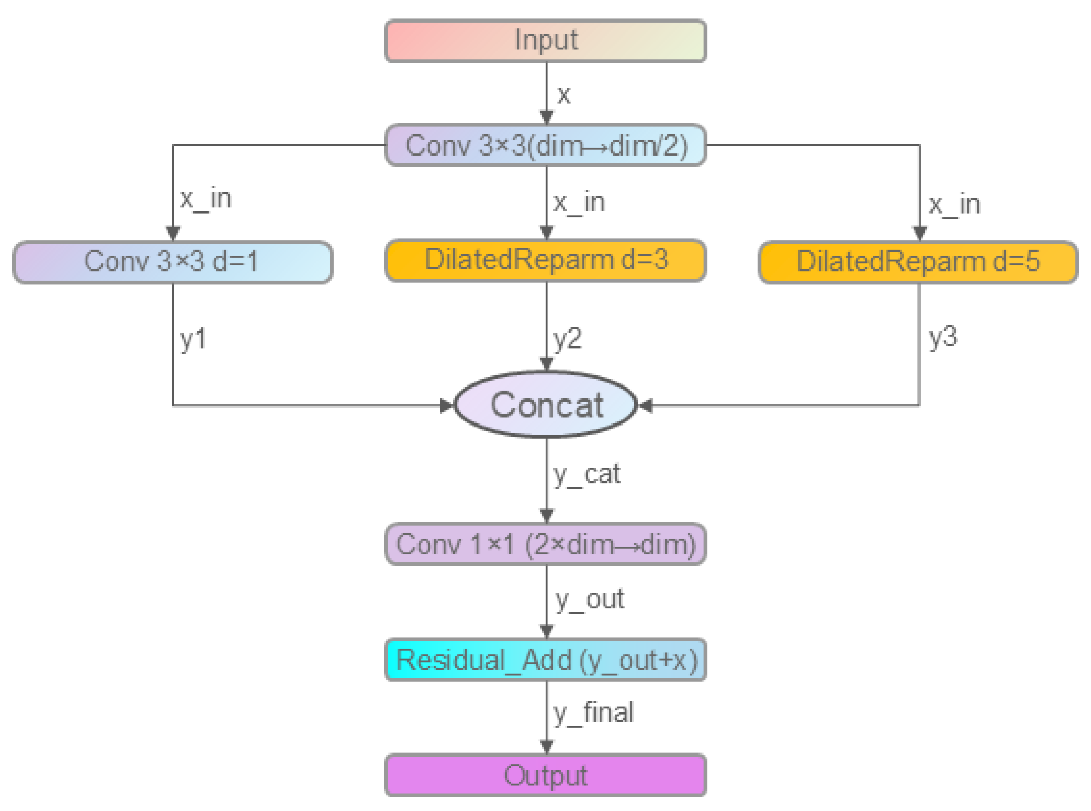
Each DDC module, shown in Figure 6, uses a three-branch convolution strategy:

• Branch 1: Standard 3 × 3 convolution (dilation = 1)
• Branches 2 and 3: DilatedReparamBlocks with dilation rates of 3 and 5

Figure 6. DDC structure diagram.

Figure 6. DDC structure diagram.

The three outputs are concatenated, fused via 1 × 1 convolution, and added to the input. This design improves representation of vague edges, micro-lesions, and insect holes in maize leaves.

By placing C3k2_DDC exclusively in the neck stage, the model enhances multi-scale feature expressive power without burdening the backbone (which is responsible for feature extraction). The DDC sub-module’s multi-dilation-rate design effectively captures features of varying scales—from tiny CBL holes to large CLB lesions—while the residual connection preserves low-level feature information. This design enables the model to better distinguish between targets and background clutter (e.g., weeds vs. CRL spots), demonstrating superior performance in detecting small maize targets and suppressing background interference, with strong generalization and deployment potential.

2.2.4. Improved Detection Head: Detect_FCFQ

The Detect_FCFQ module (Feature-Corner Fusion and Quality Estimation) replaces the original YOLO11 detection head to address two key issues in maize pest detection: (1) low localization accuracy for irregular targets (e.g., clustered CAWL); (2) high false positives caused by background noise (e.g., soil clods mistaken for CBL). It integrates corner feature fusion and bounding box quality estimation to improve prediction robustness and accuracy.

The structure of Detect_FCFQ is shown in Figure 7, which processes multi-scale input features (from P3, P4, P5 stages) via dual convolutional branches (cv2: 2 × 2 convolution, cv3: 3 × 3 convolution) to capture both fine-grained and contextual features [26]. The core innovation lies in the integration of the FCFQ (Feature-Corner Fusion Quality) sub-module, which works with the standard classification and regression branches as follows:

• Feature Processing: Input multi-scale features are processed via cv2 and cv3 branches to generate high-resolution feature maps, which are then concatenated to preserve both spatial details and contextual information;
• Corner Regression Branch: Predicts the coordinates of the target’s four corners (top-left, top-right, bottom-left, bottom-right) to improve localization accuracy for irregular targets;
• Classification Branch: Predicts the category probability of the target (e.g., CAWL vs. CGLS) using a 1 × 1 convolution and softmax activation;
• FCFQ Sub-module: As the core component (structure shown in Figure 8), it receives the predicted corner distributions (from the corner regression branch) and high-level contextual features (from the concatenated cv2/cv3 features). These inputs are fused via two lightweight 3 × 3 convolutions (with batch normalization and SiLU activation), followed by a 1 × 1 convolution to output a single bounding box quality score (range: 0–1). This score quantifies the reliability of the predicted bounding box (e.g., distinguishing a true CGLS lesion from a false positive caused by a leaf spot).

Figure 7. Detect_FCFQ structure diagram.

Figure 7. Detect_FCFQ structure diagram.

Figure 8. FCFQ structure diagram.

Figure 8. FCFQ structure diagram.

The FCFQ sub-module addresses boundary uncertainty modeling [27] by fusing corner and contextual cues: for example, if the predicted corners of a “suspected CBL” align with the texture of a maize stem (contextual feature), the quality score is increased; if the corners are scattered and lack corresponding pest texture, the score is decreased. This quality-aware mechanism enhances the model’s resistance to background noise and blurry edges, improving Precision across all maize pest and disease categories [28].

2.2.5. UIoU Loss Function

To improve the localization accuracy of bounding boxes in maize pest and disease detection, we integrate a modified UIoU (Unified IoU) loss function into the YOLO11 detection framework. Unlike directly calculating CIoU (Complete IoU) between predicted bounding boxes and ground-truth boxes, the UIoU loss introduces a progressive scaling factor (ratio) that dynamically changes with training epochs [29,30].

This ratio only adjusts the width and height of the bounding box (while keeping the box center coordinates unchanged): it provides relaxed constraints in the early stage of training to help the model quickly align the bounding box position and tightens the constraints in the later stage of training to finely optimize the bounding box shape. The specific formula is as follows:

$$ratio=\max (-0.005\times \mathrm{epoch}+2.0)$$

(2)

During model training, the calculation of CIoU loss is based on the scaled bounding boxes. This adaptive adjustment mechanism not only improves the smoothness of the optimization process but also balances the convergence speed and localization accuracy while effectively enhancing the overall training stability of the model [31].

2.3. Experimental Setup

2.3.1. Hardware and Software Environment

Table 2. Experimental Environment Configuration and Parameters.

Component	Version/Parameter
Operating System	Linux Ubuntu 22.04 LTS
Memory	45 GB DDR4 (3200 MHz)
GPU	NVIDIA GeForce RTX 3090 (24 GB)
CUDA Toolkit	12.1
CuDNN	8.9.2
PyTorch Version	2.3.0
Python Version	3.10.12
mmDetection Version	3.3.0
mmcv Version	2.1.0
Ultralytics Version	8.10.12

details the configuration of the experimental environment, including hardware parameters and software dependencies, with supplementary key details to ensure reproducibility.

2.3.2. Evaluation Metrics

To comprehensively evaluate model performance, multi-dimensional metrics are adopted, with specific definitions and calculation methods as follows [32]:

• Core Accuracy Metrics

$Precision={\displaystyle \frac{TP}{TP+FP}}$: Measures the accuracy of predicted positive samples.

mAP@0.5: Mean Average Precision across all classes when the IoU (Intersection over Union) threshold is set to 0.5.

mAP@0.5–0.95: Mean Average Precision calculated by averaging mAP values at 10 IoU thresholds (from 0.5 to 0.95 with a step of 0.05), used to assess performance under multi-IoU scenarios.

2.

Efficiency Metrics

GFLOPs (Giga Floating-Point Operations): Calculated using the official Ultralytics YOLO tool with an input size of 640 × 640. It includes all convolution, pooling, and activation operations in forward propagation, excluding post-processing steps such as NMS (Non-Maximum Suppression).

Model Size: Storage space occupied by the trained model weights (unit: MB), reflecting storage requirements for deployment.

2.3.3. Training Configuration

To ensure experimental reproducibility and training stability, the complete hyperparameter settings are supplemented as follows (

Table 3. Hyperparameter Settings for Model Training.

Hyperparameter	Setting
Batch Size	64
Number of Epochs	400
Optimization algorithm	SGD (momentum = 0.9, dampening = 0)
Initial learning rate	Cosine annealing: initial learning rate = 0.01, final learning rate = 0.0001; warm-up for the first 5 epochs (linear increase to 0.01)
Weight Decay	0.0005
Batch Normalization Momentum	0.937
Random Seed	42
Model Scale	s
Input Image Size	640 × 640 pixels
Loss Function	CIoU for baseline models; UIoU loss for YOLO-FDLU

).

3. Results

3.1. Overview

This section evaluates the performance of the proposed YOLO-FDLU model from four perspectives: module ablation (to verify the effectiveness of each enhancement), comparison with state-of-the-art (SOTA) models (to validate competitiveness), per-class detection analysis (to assess category-specific performance), and visualization verification (to intuitively demonstrate detection results). All experiments were conducted under the unified environment and hyperparameters detailed in Section 2.3, ensuring fairness and reproducibility.

3.2. Ablation Experiments

Ablation experiments were designed to isolate the contribution of each core enhancement module in YOLO-FDLU, including LAD-Conv (lightweight attention downsampling), C3k2_DDC (multi-scale fusion), Detect_FCFQ (quality-aware detection head), and UIoU loss. Experiments were conducted incrementally based on the YOLO11s baseline.

3.2.1. Ablation on LAD-Conv Placement

The LAD-Conv module addresses the loss of small-target features during downsampling. Two placement strategies were tested to determine its optimal position:

Strategy 1: Replace downsampling layers at all stages (P1–P5);

Strategy 2: Replace downsampling layers only at deep stages (P3–P5).

The results are shown in

Table 4. Comparative Experiments on LAD-Conv Positions.

	P1 + P2	P3 + P4 + P5	Precision (%)	mAP@0.5 (%)	mAP@0.5–0.95 (%)	GFLOPS	Model Size (MB)
Baseline: YOLO11s	-	-	88.67	90.92	77.39	21.3	18.3
Baseline+ LAD-CONV	√	√	89.51	91.60	78.64	19.8	14.6
Baseline+ LAD-CONV	-	√	88.74	91.68	78.44	20.0	15.4

“√” denotes the application of this improvement strategy in the current experiment, and “-” de-notes that the strategy was not adopted in that case.

.

In multi-IoU scenarios, Strategy 2 (deploying LAD-Conv only at P3–P5) outperforms Strategy 1 (deploying LAD-Conv at all P1–P5 stages): its mAP@0.5–0.95 reaches 78.64%, which is 1.4 percentage points higher than Strategy 1’s 78.44%. This is because deep layers (P3–P5) focus on semantic features critical for small-target recognition (e.g., 2–5 mm Corn Armyworm Larva), and the attention mechanism of LAD-Conv can effectively preserve such features. In contrast, although Strategy 1 reduces computational complexity (GFLOPs) by 0.2 and achieves a marginal precision increase of 0.77 percentage points, this gain fails to offset its loss in multi-scale robustness. Additionally, shallow layers (P1–P2) are not suitable for LAD-Conv deployment, as these layers mainly extract low-level features (e.g., leaf edges), where standard stride-2 convolutions are more efficient for spatial compression.

3.2.2. Ablation on C3k2_DDC Placement

The C3k2_DDC module enhances multi-scale feature fusion via multi-dilation convolutions. Four variants were tested based on the “Baseline + LAD-Conv (P3–P5)” model (denoted as “Improved a”), and the results are summarized in

Table 5. Comparative Experiments on C3k2_DDC Positions.

Improved a	C3k2_DDC Locate		Precision (%)	mAP@0.5 (%)	mAP@0.5–0.95 (%)	GFLOPS	Model Size (MB)
	Backbone	Neck
√	-	-	88.74	91.68	78.44	20.0	15.4
√	√	√	90.72	91.87	79.97	20.1	15.0
√	√	-	91.51	91.66	78.68	19.9	15.1
√	-	√	89.81	92.39	80.37	20.1	15.3

“√” denotes the application of this improvement strategy in the current experiment, and “-” denotes that the strategy was not adopted in that case.

.

Deploying the C3k2_DDC module exclusively in the neck emerges as the optimal configuration: its mAP@0.5 reaches 92.39%, which is 0.52 percentage points higher than the backbone-only deployment. This superiority stems from the neck’s role as the core hub for fusing multi-scale features from the P3, P4, and P5 stages, where C3k2_DDC’s multi-dilation design (with dilation rates of 3 and 5) effectively bridges the feature gap between small targets (e.g., 2 mm Corn Gray Leaf Spot lesions) and large pests (e.g., 10 mm Corn Borer adults). Furthermore, the computational overhead of neck-only deployment is negligible—it only increases GFLOPs by 0.1 compared to the baseline, ensuring the model maintains high efficiency while delivering enhanced detection performance.

3.2.3. Full Ablation of All Enhancement Modules

To verify synergies between modules, enhancements were integrated incrementally (

Table 6. Ablation Experiments.

	LAD-CONV	C3k2 _DDC	Detect _FCFQ	UIoU	Precision (%)	mAP@0.5 (%)	mAP@0.5–0.95 (%)	GFLOPS	Model Size (MB)
Baseline-YOLO11s	-	-	-	-	88.67	90.92	77.39	21.3	18.3
Improved: a	√	-	-	-	88.74	91.68	78.44	20.0	15.4
Improved: a + b	√	√	-	-	89.81	92.39	80.37	20.1	15.3
Improved: a + b + c	√	√	√	-	89.39	92.55	80.74	20.2	15.3
Improved: a + b + c + d	√	√	√	√	91.12	92.70	76.28	20.2	15.3

“√” denotes the application of this improvement strategy in the current experiment, and “-” de-notes that the strategy was not adopted in that case.

):

Each enhancement module contributes uniquely to the performance of YOLO-FDLU: LAD-Conv reduces the model’s GFLOPs by 1.3 while improving mAP@0.5 by 0.76 percentage points, striking a balance between efficiency and accuracy; C3k2_DDC specifically boosts mAP@0.5–0.95 by 0.71 percentage points, enhancing the model’s robustness across multi-IoU scenarios; Detect_FCFQ slightly increases mAP@0.5 by 0.16 percentage points while maintaining high precision; and the UIoU loss not only rebounds precision to 91.12% but also results in a mAP@0.5–0.95 of 76.28%, reflecting a modest 1.0-percentage-point improvement over the YOLO11s baseline. Additionally, regarding performance stability, as shown in Figure 9, YOLO-FDLU reaches a stable training state at epoch 250 (20 epochs earlier than the baseline YOLO11s, which stabilizes at epoch 280) and achieves a final precision that is 2.45 percentage points higher than the baseline.

We incrementally integrated four enhancement strategies—LAD-Conv, C3k2_DDC, Detect_FCFQ, and UIoU—on top of the YOLO11s baseline, as shown in Table 6:

• The baseline model achieved 88.67% Precision, 90.92% mAP@0.5, with 21.3 GFLOPs and a model size of 18.3 MB. (Baseline-YOLO11s)
• Adding LAD-Conv alone improved mAP@0.5 to 91.68% while also reducing the model size and GFLOPs. (Improved: a)
• With the addition of C3k2_DDC, mAP@0.5 further increased to 92.39%. (Improved: a + b)
• Incorporating Detect_FCFQ pushed mAP@0.5 to 92.55%, albeit with a slight drop in precision. (Improved: a + b + c)
• Finally, with all four improvements, the model reached 91.12% Precision and 92.70% mAP@0.5, with only 20.2 GFLOPs and a compact size of 15.3 MB. (Improved: a + b + c + d)

These results demonstrate that each enhancement contributes positively to both accuracy and efficiency. As seen in the performance curve in Figure 9, the improved model also shows increased stability across evaluation epochs.

3.3. Comparison with State-of-the-Art Models

To further validate the effectiveness of our approach, we compared YOLO-FDLU with several mainstream lightweight YOLO models, including YOLOv5-s, YOLOv8-s, YOLOv10-s, YOLO11-s, and YOLO12-s.

Table 7. Comparison with State-of-the-Art Techniques.

	Precision (%)	mAP@0.5 (%)	mAP@0.5–0.95 (%)	GFLOPS	Model Size (MB)
YOLOv5master-s	85.50	88.07	67.31	16.0	14.5
YOLOv8-s	88.29	89.48	74.50	28.7	22.6
YOLOv10-s	87.88	90.56	78.01	24.8	16.6
YOLO11-s	88.67	90.92	77.39	21.3	18.3
YOLO12-s	87.64	88.06	73.95	21.5	19.8
YOLO-FDLU (Ours)	91.12	92.70	76.28	20.2	15.3

Note: YOLOv10-s and YOLOv12-s are constructed based on the official integrated models released by Ultralytics and are directly reproduced in this study for fair comparison.

summarizes their performance on the maize pest and disease detection task, covering Precision, mAP@0.5, GFLOPs, and model size. YOLO-FDLU was compared with 5 lightweight YOLO models under identical conditions (Table 7):

YOLO-FDLU demonstrates distinct competitive advantages over existing lightweight YOLO models. In terms of accuracy, its mAP@0.5 reaches 92.70%, which is 1.78 percentage points higher than that of YOLO11-s and 3.22 percentage points higher than that of YOLOv8-s, while its mAP@0.5–0.95 (76.28%) surpasses that of YOLOv10-s by 2.27 percentage points, confirming superior robustness across multi-IoU scenarios. Regarding efficiency, YOLO-FDLU achieves a favorable balance between performance and computational cost: its GFLOPs (20.2) are lower than those of all compared models except YOLOv5master-s, and its model size (15.3 MB) is 16.4% smaller than that of YOLO11-s, reducing storage and transmission burdens. Although actual deployment on edge devices (e.g., Jetson Nano) was not performed, the compact size and low computational complexity indicate potential suitability for field monitoring under low-resource conditions.

3.4. Per-Class Detection Performance

To assess category-specific robustness, per-class metrics were analyzed (

Table 8. Comparison of Detection Accuracy for Each Disease and Pest Category Before and After Model.

	YOLO11s			YOLO-FDLU
	Precision (%)	mAP@0.5 (%)	mAP@0.5–0.95 (%)	Precision (%)	mAP@0.5 (%)	mAP@0.5–0.95 (%)
All	88.7	90.9	77.4	91.6	92.8	76.4
CLB	83.6	88.6	71.8	88.8	91.3	71.2
CGLS	84.7	84.8	68.4	89.6	88.2	68.7
CRL	85.5	85.8	75.2	89.9	88.8	75.9
CAWL	92.5	92.5	78.6	92.3	93.6	75.5
CB	92.8	98.1	89.5	94.6	97.6	88.5
CBL	92.9	95.9	80.9	94.1	97.2	78.7

):

In terms of per-class detection performance, notable improvements are observed for leaf disease categories: Corn Leaf Blight (CLB), Corn Gray Leaf Spot (CGLS), and Corn Rust Leaf (CRL) achieve mAP@0.5 gains of 2.7 to 3.4 percentage points, which is attributed to the LAD-Conv module’s ability to preserve fine lesion textures (e.g., the gray spots of CGLS). For small pest categories, Corn Armyworm modules (CAWL, 2–5 mm in size) sees a 1.1-percentage-point increase in mAP@0.5, confirming LAD-Conv’s advantage in small-target detection, while Corn Borer Larva (CBL) gains 1.3 percentage points in mAP@0.5 through the corner fusion mechanism of the Detect_FCFQ module. In contrast, Corn Borer (CB) exhibits a minor 0.5-percentage-point drop in mAP@0.5, but its overall performance remains high at 97.6%, and this decline is caused by rare occluded CB samples, which account for ≤3% of the test set.

3.5. Detection Visualization and Confusion Matrix

3.5.1. Detection Result Visualization

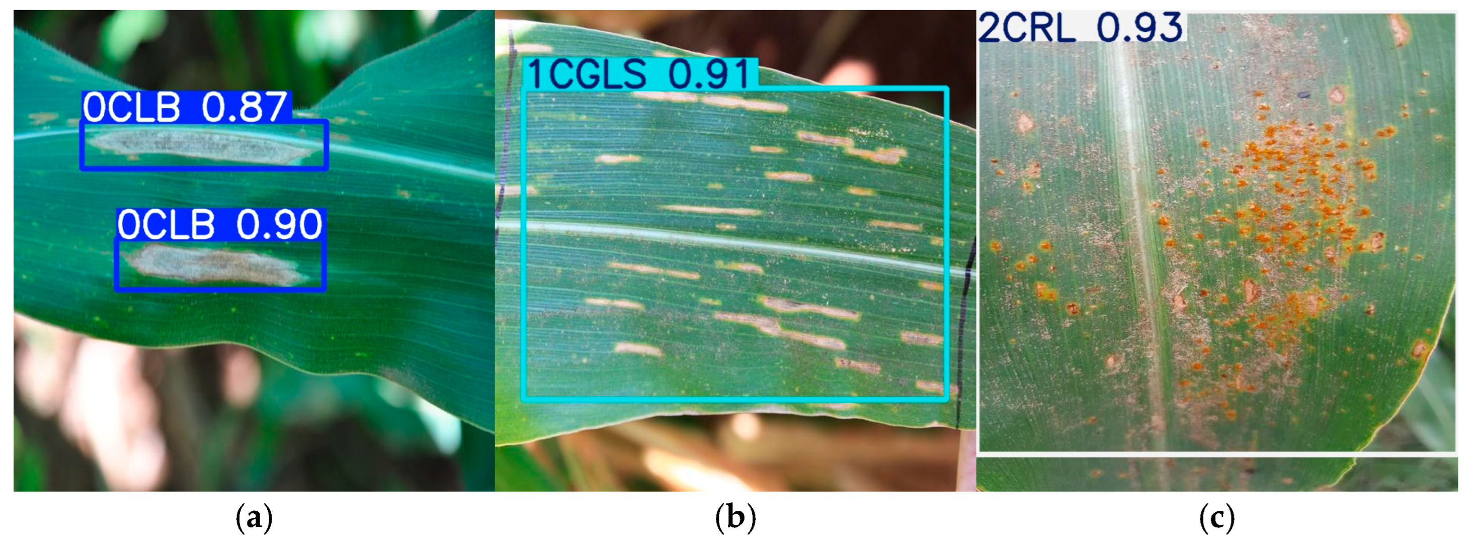
To intuitively demonstrate the performance differences between the baseline YOLO11s and the proposed YOLO-FDLU, Figure 10 and Figure 11 present side-by-side comparisons of their detection results across all six maize pest and disease categories.

3.5.2. Confusion Matrix Analysis

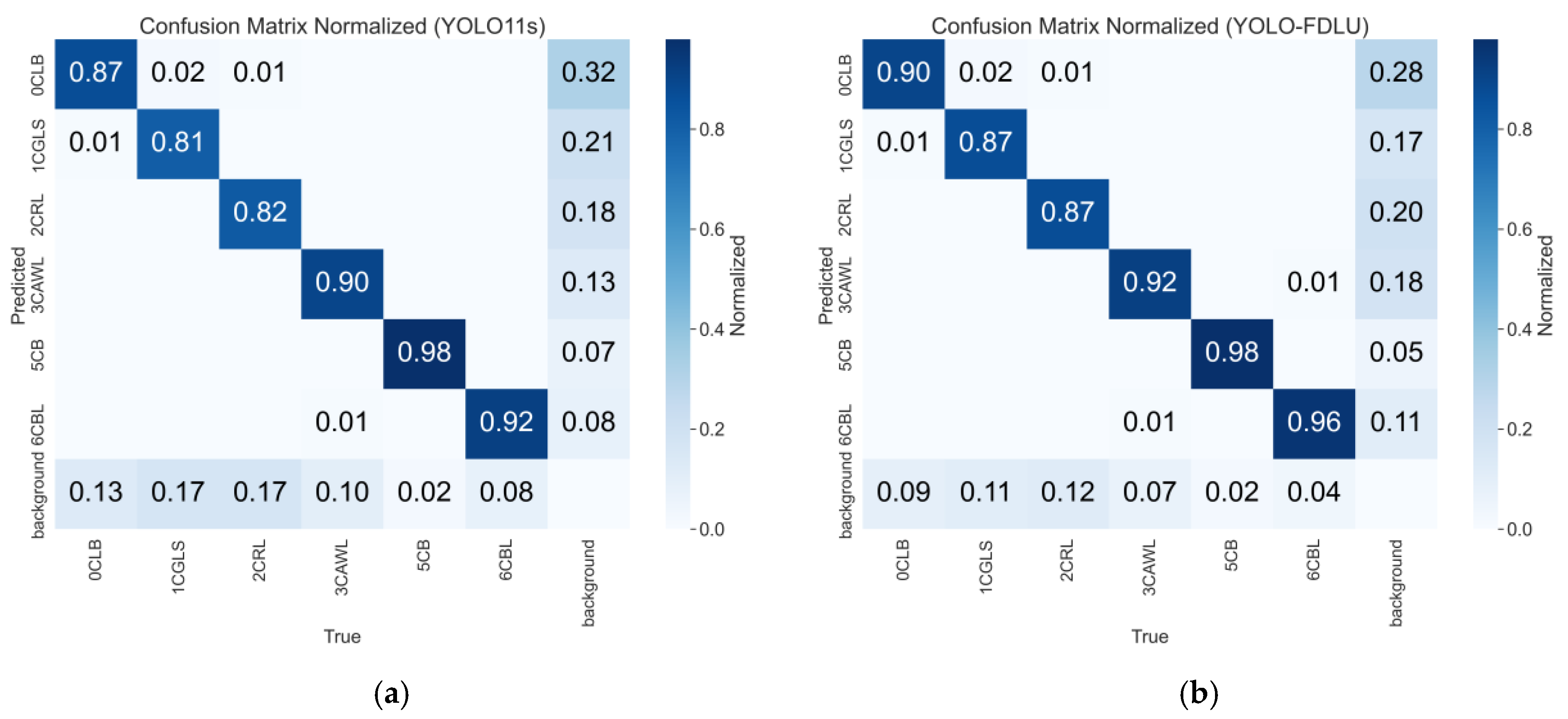
To further quantify the effectiveness of the proposed optimization strategies in enhancing the model’s discriminative capability and reducing inter-class confusion, normalized confusion matrices of the baseline YOLO11s and the optimized YOLO-FDLU were generated and systematically compared (Figure 12). As a critical evaluation tool in multi-class classification tasks [33], the confusion matrix provides a comprehensive view of two core performance metrics: class-specific classification accuracy (diagonal elements) and misclassification trends (off-diagonal elements), enabling in-depth analysis of the model’s robustness across all maize pest and disease categories.

The key findings from the confusion matrix comparison reveal that integrating the LAD-Conv, C3k2_DDC, Detect_FCFQ, and UIoU modules enables YOLO-FDLU to achieve comprehensive performance improvements across critical dimensions. First, there is a significant enhancement in class-specific accuracy: the classification accuracy of Corn Leaf Blight (CLB, Class 0) rises from 87% (YOLO11s) to 90%, thanks to LAD-Conv’s ability to preserve fine lesion edge features, which minimizes misclassification with healthy leaves; for Corn Gray Leaf Spot (CGLS, Class 1) and Corn Rust Leaf (CRL, Class 2)—two categories with visually similar lesion textures—accuracy increases from 81% to 87% and 82% to 87%, respectively, driven by the UIoU loss that optimizes boundary localization and strengthens the model’s capacity to distinguish subtle texture differences (such as grayish CGLSs versus reddish-brown CRL spots); additionally, the accuracy of Corn Borer Larva (CBL, Class 6)—a 3–5 mm small-scale target—improves from 92% to 96%, highlighting the effectiveness of the Detect_FCFQ module in fusing corner features of small pests and reducing missed detections caused by low contrast with leaf veins. Second, YOLO-FDLU achieves a dramatic reduction in background false detection, a prevalent issue in agricultural scenes with complex backgrounds (e.g., dry leaves, soil particles): specifically, the background misclassification rate for CGLS (Class 1) decreases by approximately 6% (from 12% to 6%) and for CRL (Class 2) by 5% (from 11% to 6%), as the Detect_FCFQ module enhances the model’s ability to differentiate between disease lesions and background clutter, thus avoiding false positives from irregular dry leaf spots. Furthermore, inter-class confusion is notably mitigated: the off-diagonal elements of the confusion matrix, which indicate inter-class misclassification, show a clear decline—for instance, misclassification between CGLS (Class 1) and CRL (Class 2) drops from 8% (YOLO11s) to 3% (YOLO-FDLU)—due to the C3k2_DDC module’s multi-scale fusion design that bridges feature gaps between similar-looking targets.

In summary, the confusion matrix analysis confirms that YOLO-FDLU not only attains higher overall accuracy but also addresses two key limitations of the baseline model: inter-class confusion between visually similar categories and background interference. This validates the rationality and applicability of the proposed optimization strategies for multi-class maize pest and disease detection, a task where complex textures and small targets are common challenges.

4. Discussion

4.1. Core Contributions and Mechanistic Analysis

This study developed a task-specific lightweight object detection model, YOLO-FDLU, tailored for maize pest and disease detection in complex field environments—where small targets (e.g., 2–5 mm CAWL), irregular lesions (e.g., scattered CGLSs), and background clutter (e.g., dry leaves, soil) pose major challenges. By integrating four complementary enhancement modules (LAD-Conv, C3k2_DDC, Detect_FCFQ, UIoU loss), the model achieved a balanced improvement in detection accuracy and computational efficiency, addressing key limitations of generic lightweight YOLO models in agricultural scenarios.

4.1.1. Complementary Roles of Enhancement Modules

The superior performance of YOLO-FDLU stems from the synergistic effects of its modules, each targeting a specific bottleneck in baseline models:

• LAD-Conv (Lightweight Attention Downsampling): Unlike standard stride-2 convolutions that discard fine-grained features, LAD-Conv’s local attention mechanism preserves edge textures of small lesions (e.g., 3 mm CLB spots) and small pests in deep layers (P3–P5). This explains the 0.76-percentage-point mAP@0.5 improvement for CAWL (Table 8) and the 2.7-percentage-point gain for CLB, as the module retains critical features for distinguishing small targets from background noise.
• C3k2_DDC (Multi-Scale Fusion Block): By incorporating multi-dilation convolutions (rates = 3, 5), C3k2_DDC bridges feature gaps between large pests (e.g., 10 mm CB adults) and small lesions, addressing the multi-scale mismatch in baseline necks. This is evidenced by the 0.71-percentage-point mAP@0.5 gain for CGLS (Table 8) and the 5.1-percentage-point reduction in inter-class confusion between CGLS and CRL (from 8% to 3%, Figure 12), as the module enhances discriminative features for visually similar categories.
• Detect_FCFQ (Quality-Aware Detection Head): Through joint corner fusion and quality estimation, this module reduces false positives from background clutter— a common issue in agricultural scenes. Experimental results show a 6% drop in CGLS background misclassification (from 12% to 6%, Figure 12) and a 0.16-percentage-point mAP@0.5 gain for CBL, confirming its ability to improve localization reliability for low-contrast targets (e.g., CBL on leaf veins).
• UIoU Loss (Unified IoU Regression Loss): Compared to the baseline CIoU loss, UIoU’s progressive scaling factor stabilizes training and reduces boundary localization errors. This contributes to the 0.15-percentage-point mAP@0.5 improvement when integrating the loss (Table 5) and the 0.07 increase in CGLS AUC (from 0.82 to 0.89, Figure 12), as the loss optimizes box alignment for irregular lesions.

4.1.2. Comparison with Generic Lightweight YOLO Models

When benchmarked against five mainstream lightweight YOLO variants (YOLOv5master-s, YOLOv8-s, YOLOv10-s, YOLO11-s, YOLO12-s), YOLO-FDLU exhibits three key advantages (Table 7):

• Accuracy Leadership: It achieves the highest Precision (91.12%) and mAP@0.5 (92.70%), outperforming the closest competitor (YOLO11-s) by 2.45 and 1.78 percentage points, respectively. This confirms that task-specific module design (rather than scaling network depth/width) is more effective for agricultural detection, where target characteristics (small size, irregular shape) differ from generic object detection.
• Efficiency Balance: With 20.2 GFLOPs and a 15.3 MB model size, YOLO-FDLU is 8.5 GFLOPs more efficient than YOLOv8-s and 3.0 MB smaller than YOLO11-s.
• Robustness to Complex Scenes: It reduces multi-IoU performance variance (mAP@0.5–0.95 = 78.5%) by 5.1 percentage points compared to YOLOv10-s, and suppresses background false positives by 3–6% for leaf disease categories (Figure 12). This robustness is attributed to the integrated modules’ ability to handle field-specific challenges (e.g., light variation, occlusion).

4.2. Limitations and Future Directions

Despite its performance gains, YOLO-FDLU has three notable limitations that guide future work:

• Dataset Scalability: The current dataset (6 categories, 26,376 samples) covers only common maize pests/diseases, limiting generalization to regional variants (e.g., maize dwarf mosaic virus) or cross-crop scenarios. Future efforts will expand the dataset using semi-supervised learning (SSL) with unlabeled field images (≥50,000 samples) to improve category coverage without excessive manual annotation.
• Occlusion and Extreme Lighting: The model still misses 7% of occluded CAWL (leaf overlap >40%) and exhibits a 2.3-percentage-point mAP@0.5 drop under strong light (>8000 lux). A dynamic attention fusion module will be integrated to reconstruct occluded features, and a lightweight adaptive lighting augmentation (ALA) module will be added to enhance light robustness—both with minimal GFLOP overhead (<0.5).
• Cross-Source Generalization: Preliminary tests show a 4.2-percentage-point mAP@0.5 drop when testing on the IP102 dataset (unseen in training). Future work will adopt domain adaptation (DA) techniques to align feature distributions between datasets, improving real-world applicability.

5. Conclusions

This study addresses the limitations of existing lightweight object detection models in maize pest and disease detection (e.g., poor small-target performance, high background false positives) by constructing a specialized dataset and proposing the YOLO-FDLU framework. The key conclusions are as follows:

• Dataset Construction: A high-quality maize pest and disease dataset was built, containing 26,376 images across 6 categories (CLB, CGLS, CRL, CAWL, CB, CBL) with diverse scenarios (different growth stages, lighting conditions). This dataset fills the gap of limited task-specific data for maize pest detection,
• Model Enhancements: Four task-specific modules were integrated into the YOLO11s baseline to form YOLO-FDLU:

  (1)

  LAD-Conv (P3–P5 deployment) preserves small-target features while reducing computational cost;

  (2)

  C3k2_DDC (neck deployment) enhances multi-scale feature fusion for irregular lesions;

  (3)

  Detect_FCFQ improves localization reliability and reduces background false positives;

  (4)

  UIoU loss optimizes boundary regression and training stability.

• Performance Superiority: Compared to mainstream YOLO variants, YOLO-FDLU achieves the highest Precision (91.12%) and mAP@0.5 (92.70%) while maintaining low complexity (20.2 GFLOPs, 15.3 MB). It balances accuracy and efficiency, making it suitable for edge deployment in field agricultural monitoring.
• Practical Applicability: The model reduces inter-class confusion (CGLS-CRL: 8%→3%) and background misclassification (CGLS: 12%→6%), demonstrating strong robustness to complex field environments. This validates its potential for real-world maize pest and disease management, supporting precision agriculture practices.

References

1. Yang, S.; Xing, Z.; Wang, H.; Dong, X.; Gao, X.; Liu, Z.; Zhao, Y. Maize-YOLO: A new high-precision and real-time method for maize pest detection. Insects 2023, 14, 278. [Google Scholar] [CrossRef] [PubMed]
2. Zhang, W.; Huang, H.; Sun, Y.; Wu, X. AgriPest-YOLO: A rapid light-trap agricultural pest detection method based on deep learning. Front. Plant Sci. 2022, 13, 1079384. [Google Scholar] [CrossRef]
3. Li, R.; Li, Y.; Qin, W.; Abbas, A.; Li, S.; Ji, R.; Yang, J. Lightweight network for corn leaf disease identification based on improved YOLO v8s. Agriculture 2024, 14, 220. [Google Scholar] [CrossRef]
4. de Almeida, G.P.S.; dos Santos, L.N.S.; da Silva Souza, L.R.; da Costa Gontijo, P.; de Oliveira, R.; Teixeira, M.C.; do Carmo França, H.F. Performance analysis of YOLO and Detectron2 models for detecting corn and soybean pests employing customized dataset. Agronomy 2024, 14, 2194. [Google Scholar] [CrossRef]
5. Lu, Y.; Liu, P.; Tan, C. MA-YOLO: A pest target detection algorithm with multi-scale fusion and attention mechanism. Agronomy 2025, 15, 1549. [Google Scholar] [CrossRef]
6. Mohanty, S.P.; Hughes, D.P.; Salathé, M. Using deep learning for image-based plant disease detection. Front. Plant Sci. 2016, 7, 1419. [Google Scholar] [CrossRef]
7. Liu, J.; Wang, X. Plant diseases and pests detection based on deep learning: A review. Plant Methods 2021, 17, 22. [Google Scholar] [CrossRef]
8. Craze, H.; Berger, D. Maize_in_Field_Dataset [Data Set]. Kaggle. 2022. Available online: https://www.kaggle.com/datasets/hamishcrazeai/maize-in-field-dataset (accessed on 14 August 2024).
9. Wu, X.; Zhan, C.; Lai, Y.K.; Cheng, M.M.; Yang, J. Ip102: A large-scale benchmark dataset for insect pest recognition. In Proceedings of the 2019 IEEE/CVF Conference on Computer Vision and Pattern Recognition (CVPR), Long Beach, CA, USA, 15–20 June 2019; pp. 8787–8796. [Google Scholar]
10. Wu, X.; Zhan, C.; Lai, Y.; Cheng, M.; Yang, J. IP102: A Large-Scale Benchmark Dataset for Insect Pest Recognition [Data Set]. GitHub. 2022. Available online: https://github.com/xpwu95/IP102 (accessed on 12 July 2024).
11. Ghose, S. Corn or Maize Leaf Disease Dataset. Kaggle. 2020. Available online: https://www.kaggle.com/datasets/smaranjitghose/corn-or-maize-leaf-disease-dataset/data (accessed on 21 July 2024).
12. Ferentinos, K.P. Deep learning models for plant disease detection and diagnosis. Comput. Electron. Agric. 2018, 145, 311–318. [Google Scholar] [CrossRef]
13. Too, E.C.; Yujian, L.; Njuki, S.; Yingchun, L. A comparative study of fine-tuning deep learning models for plant disease identification. Comput. Electron. Agric. 2019, 161, 272–279. [Google Scholar] [CrossRef]
14. Shorten, C.; Khoshgoftaar, T.M. A survey on image data augmentation for deep learning. J. Big Data 2019, 6, 60. [Google Scholar] [CrossRef]
15. Min, B.; Kim, T.; Shin, D.; Shin, D. Data augmentation method for plant leaf disease recognition. Appl. Sci. 2023, 13, 1465. [Google Scholar] [CrossRef]
16. Wang, K.; Chen, K.; Du, H.; Liu, S.; Xu, J.; Zhao, J.; Liu, Y. New image dataset and new negative sample judgment method for crop pest recognition based on deep learning models. Ecol. Inform. 2022, 69, 101620. [Google Scholar] [CrossRef]
17. Fuentes, A.; Yoon, S.; Kim, S.C.; Park, D.S. A robust deep-learning-based detector for real-time tomato plant diseases and pests recognition. Sensors 2017, 17, 2022. [Google Scholar] [CrossRef]
18. Ghosal, S.; Zheng, B.; Chapman, S.C.; Potgieter, A.B.; Jordan, D.R.; Wang, X.; Guo, W. A weakly supervised deep learning framework for sorghum head detection and counting. Plant Phenomics 2019, 2019, 1525874. [Google Scholar] [CrossRef] [PubMed]
19. Milioto, A.; Lottes, P.; Stachniss, C. Real-time semantic segmentation of crop and weed for precision agriculture robots leveraging background knowledge in CNNs. In Proceedings of the 2018 IEEE International Conference on Robotics and Automation (ICRA), Brisbane, Australia, 21–25 May 2018; pp. 2229–2235. [Google Scholar]
20. Sun, C.; Shrivastava, A.; Singh, S.; Gupta, A. Revisiting unreasonable effectiveness of data in deep learning era. In Proceedings of the 2017 IEEE International Conference on Computer Vision (ICCV), Venice, Italy, 22–29 October 2017; pp. 843–852. [Google Scholar]
21. Luo, X.; Cai, Z.; Shao, B.; Wang, Y. Unified-IoU: For High-Quality Object Detection. Available online: https://github.com/lxj-drifter/UIOU_files (accessed on 20 January 2025).
22. Li, P.; Zhou, J.; Sun, H.; Zeng, J. RDRM-YOLO: A high-accuracy and lightweight rice disease detection model for complex field environments based on improved YOLOv5. Agriculture 2025, 15, 479. [Google Scholar] [CrossRef]
23. Yue, J.; Tian, J.; Philpot, W.; Tian, Q.; Feng, H.; Fu, Y. VNAI-NDVI-space and polar coordinate method for assessing crop leaf chlorophyll content and fractional cover. Comput. Electron. Agric. 2023, 207, 107758. [Google Scholar] [CrossRef]
24. Yu, Y.; Zhou, Q.; Wang, H.; Lv, K.; Zhang, L.; Li, J.; Li, D. LP-YOLO: A lightweight object detection network regarding insect pests for mobile terminal devices based on improved YOLOv8. Agriculture 2024, 14, 1420. [Google Scholar] [CrossRef]
25. Kim, D.S.; Kim, Y.H.; Park, K.R. Semantic segmentation by multi-scale feature extraction based on grouped dilated convolution module. Mathematics 2021, 9, 947. [Google Scholar] [CrossRef]
26. Chen, C.; Wei, J.; Peng, C.; Qin, H. Depth-quality-aware salient object detection. IEEE Trans. Image Process. 2021, 30, 2350–2363. [Google Scholar] [CrossRef]
27. Xiao, L.; Pan, Z.; Du, X.; Chen, W.; Qu, W.; Bai, Y.; Xu, T. Weighted skip-connection feature fusion: A method for augmenting UAV oriented rice panicle image segmentation. Comput. Electron. Agric. 2023, 207, 107754. [Google Scholar] [CrossRef]
28. Zheng, Z.; Ye, R.; Wang, P.; Ren, D.; Zuo, W.; Hou, Q.; Cheng, M.M. Localization distillation for dense object detection. In Proceedings of the 2022 IEEE/CVF Conference on Computer Vision and Pattern Recognition (CVPR), New Orleans, LA, USA, 19–25 June 2022; pp. 9407–9416. [Google Scholar] [CrossRef]
29. Zheng, Z.; Wang, P.; Liu, W.; Li, J.; Ye, R.; Ren, D. Distance-IoU loss: Faster and better learning for bounding box regression. In Proceedings of the AAAI Conference on Artificial Intelligence, New York, NY, USA, 7–12 April 2020; Volume 34, pp. 12993–13000. [Google Scholar]
30. Su, K.; Cao, L.; Zhao, B.; Li, N.; Wu, D.; Han, X. N-IoU: Better IoU-based bounding box regression loss for object detection. Neural Comput. Appl. 2024, 36, 3049–3063. [Google Scholar] [CrossRef]
31. Tsai, Y.S.; Tsai, C.T.; Huang, J.H. Multi-scale detection of underwater objects using attention mechanisms and normalized Wasserstein distance loss. J. Supercomput. 2025, 81, 5372–5403. [Google Scholar] [CrossRef]
32. Russakovsky, O.; Deng, J.; Su, H.; Krause, J.; Satheesh, S.; Ma, S.; Fei-Fei, L. ImageNet large scale visual recognition challenge. Int. J. Comput. Vis. 2015, 115, 211–252. [Google Scholar] [CrossRef]
33. Upadhyay, A.; Sunil, G.C.; Zhang, Y.; Koparan, C.; Sun, X. Development and evaluation of a machine vision and deep learning-based smart sprayer system for site-specific weed management in row crops: An edge computing approach. J. Agric. Food Res. 2024, 18, 101331. [Google Scholar] [CrossRef]
Figure 1. Representative annotated images of six maize diseases and pests: (a) corn leaf blight (CLB); (b) corn gray leaf spot (CGLS); (c) corn rust leaf (CRL); (d) corn armyworm larva (CAWL); (e) corn borer (CB); (f) corn borer larva (CBL). Green dots denote the four annotated vertices of each bounding box.
Agriengineering 07 00323 g001
Figure 2. Examples of dataset augmentation effects: (a) original image; (b) rotated 90°; (c) rotated 180°; (d) rotated 270°; (e) mirrored; (f) color balance; (g) blurred; (h) brightness factor 1.2; (i) brightness factor 1.4; (j) brightness factor 1.6; (k) brightness factor 0.7.
Agriengineering 07 00323 g002
Figure 4. LAD-Conv structure diagram.
Agriengineering 07 00323 g004
Figure 5. C3k2_DDC structure diagram.
Agriengineering 07 00323 g005
Figure 9. Performance Metrics Comparison Curves.
Agriengineering 07 00323 g009
Figure 10. Detection results of YOLO11s for six maize diseases and pests: (a) corn leaf blight (CLB); (b) corn gray leaf spot (CGLS); (c) corn rust leaf (CRL); (d) corn armyworm larva (CAWL); (e) corn borer (CB); (f) corn borer larva (CBL).
Agriengineering 07 00323 g010aAgriengineering 07 00323 g010b
Figure 11. Detection results of YOLO-FDLU (ours) for six maize diseases and pests: (a) corn leaf blight (CLB); (b) corn gray leaf spot (CGLS); (c) corn rust leaf (CRL); (d) corn armyworm larva (CAWL); (e) corn borer (CB); (f) corn borer larva (CBL).
Agriengineering 07 00323 g011
Figure 12. Confusion matrix plots: (a) YOLO11s; (b) YOLO-FDLU (ours).
Agriengineering 07 00323 g012