1. Introduction
Over the past decades, the frequency of extreme weather events during the growing season of plants, combining high light intensity and high temperatures, has increased dramatically [
1]. Light stress occurs if the plant does not get rid of the excess energy received from the bright sun. Under stress from high light intensity, reaction centres become saturated, and excess energy can irreversibly damage photosystem II (PSII) [
2]. This leads to photoinhibition—a steady decrease in the efficiency of photosynthesis [
3]. Light stress during the growing season is usually combined with heat stress. Both of these stresses have a synergistic effect on plants [
4,
5].
One of the defence mechanisms against light stress is that plant leaves change the composition of pigments that absorb light. Another defence mechanism is that chloroplasts can move to shaded areas in plant cells. There is also a defence mechanism in which plants dissipate excess light energy as heat [
6].
Light and heat stress lead to a significant decrease in plant productivity. The ability to quickly identify plant responses to stress is essential for improving crop-management practices and addressing the global food-security challenge. Therefore, an important task is to identify stress in plants quickly, using noninvasive and simple methods, over large areas. Rapid diagnosis of light stress in plants over large areas is only possible using Earth remote-sensing (ERS) data. In confined areas, e.g., in greenhouses, foil tunnels, or open plantations, proximal spectral sensors can be used for stress recording. It is generally accepted that, among different remote-sensing techniques, the use of hyperspectral survey data is the most effective for plant-stress analysis [
7]. A large number of remote hyperspectral studies were carried out on water-stress diagnostics [
7,
8,
9]. Spectral sensors proved to be effective in diagnosing stress in plants from high [
10,
11,
12] and low [
13] temperatures. It is important to diagnose all kinds of stress before the first visible symptoms appear [
14]. In this relation, there is a necessity to develop low-cost portable spectral optical sensors to accurately detect and diagnose the nature of plant stress [
15].
The pigment composition of leaves, their photosynthetic characteristics and, accordingly, their optical properties are influenced by various stress factors, e.g., highly active forms of oxygen, air pollutants, drought, high temperatures, bright light, increased levels of UV radiation and others [
16].
An evaluation of the physiological state of plants (including remote evaluations) may be performed using spectral characteristics and measurements of vegetation indices related to the contents of photosynthetic pigments [
17,
18,
19]. In this regard, it is important to develop a new vegetation index (VI) for indicating plant stress.
The mechanism of the damaging effect of light excess on plants (photoinhibition) is mediated by the generation of superoxide ion O
2*
− [
20,
21] and singlet oxygen
1O
2 [
22] that can interact with photosystem I and II elements and impair their functions. In particular, the prerequisites for photoinhibition appear, if the electron light-excitation rate (i.e., number of P680 or P700 excited states generated per time unit) exceeds the electron transfer capacity of the thylakoid electron transport chain. In this case, there is a high probability of the transfer of excited electrons to O
2, followed by the formation of reactive oxygen species, which damage PSII and accessory pigments in antennae complexes [
23], thus changing absorption spectra [
21,
22,
24].
Thus, remote-sensing tools equipped with spectral sensors can identify stress in plants as such, but it is very difficult to determine its nature. Therefore, the development of a special technique for determining the light stress of plants using spectral sensors that record passive reflection is an important task.
The aim of the study was to determine the spectral ranges that make it possible to diagnose light stress in plants. The implementation of this task was carried out in laboratory conditions, in which the influence of random factors is minimized. The data obtained may be useful for the further development of simple and low-cost multispectral cameras applicable as Earth remote-sensing (ERS) tools.
2. Materials and Methods
Ficus elastica Roxb. ex Hornem plants were selected for the light-stress studies. They were expected to be sensitive to light stress, as they are short-day shade-tolerant plants. The plants were grown in the greenhouse of the Botanical Garden of the Southern Federal University under natural light (about 100 µmol photons m−2 s−1), relative soil humidity of 60%, and a light/dark regime = 14/10 for 14 months. All the plants were of the same age.
Hyperspectral Imaging (HSI) was carried out using a Cubert UHD-185 [
25,
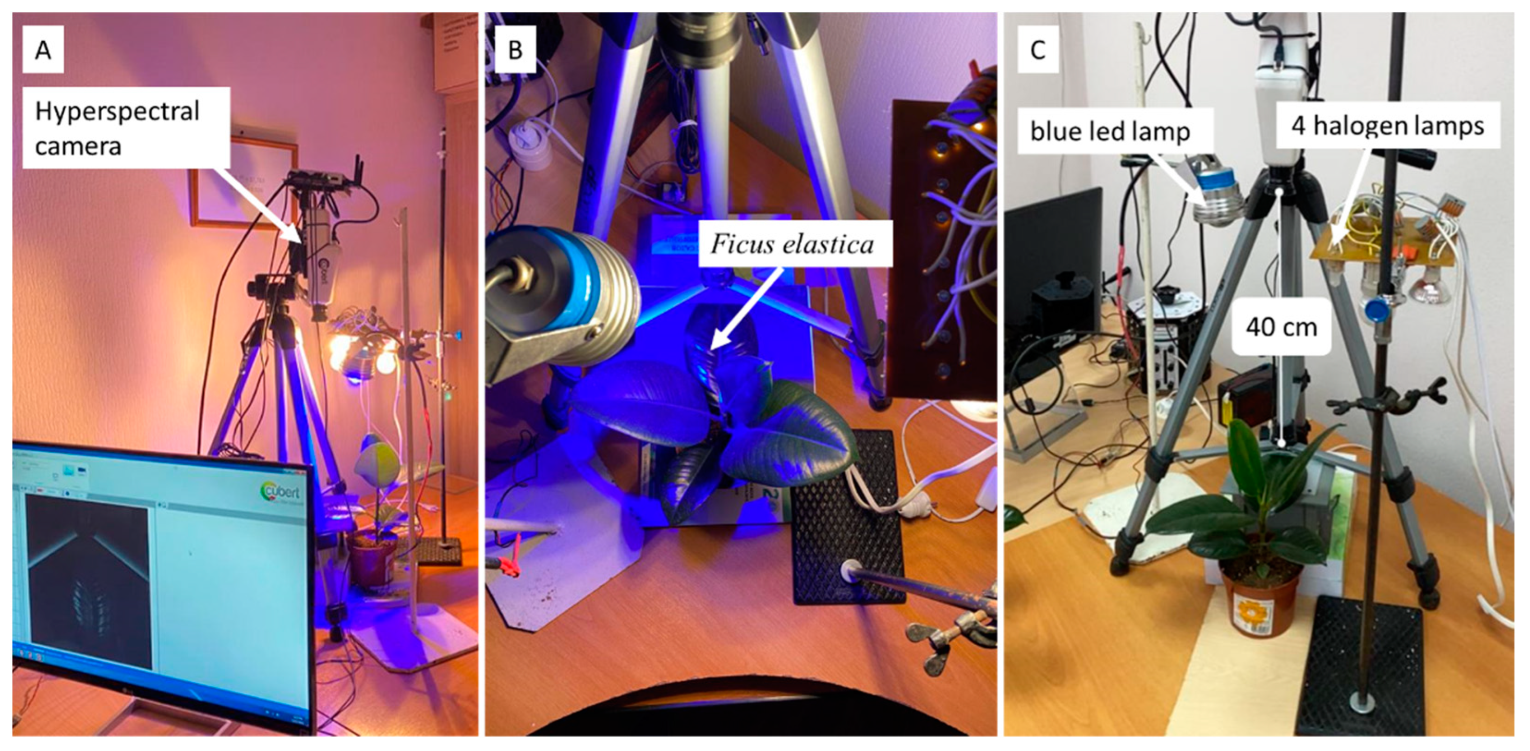
26]. The wavelength range of this hyperspectral camera is from 450 nm to 950 nm; the spectral resolution is 4 nm. The camera lens was located at a distance of 40 cm from the leaf blade of the plant and directed perpendicular to it (
Figure 1). HSI was conducted under 4 halogen lamps and 1 blue LED. The integral spectrum of the measuring light is shown in
Figure 2. Each hyperspectral image is presented as a single panchromatic image, 1000 × 1000 pixels in size and 125 spectral images, 50 × 50 pixels in size. The spatial resolution of the obtained hyperspectral data was approximately 35 mm
2.
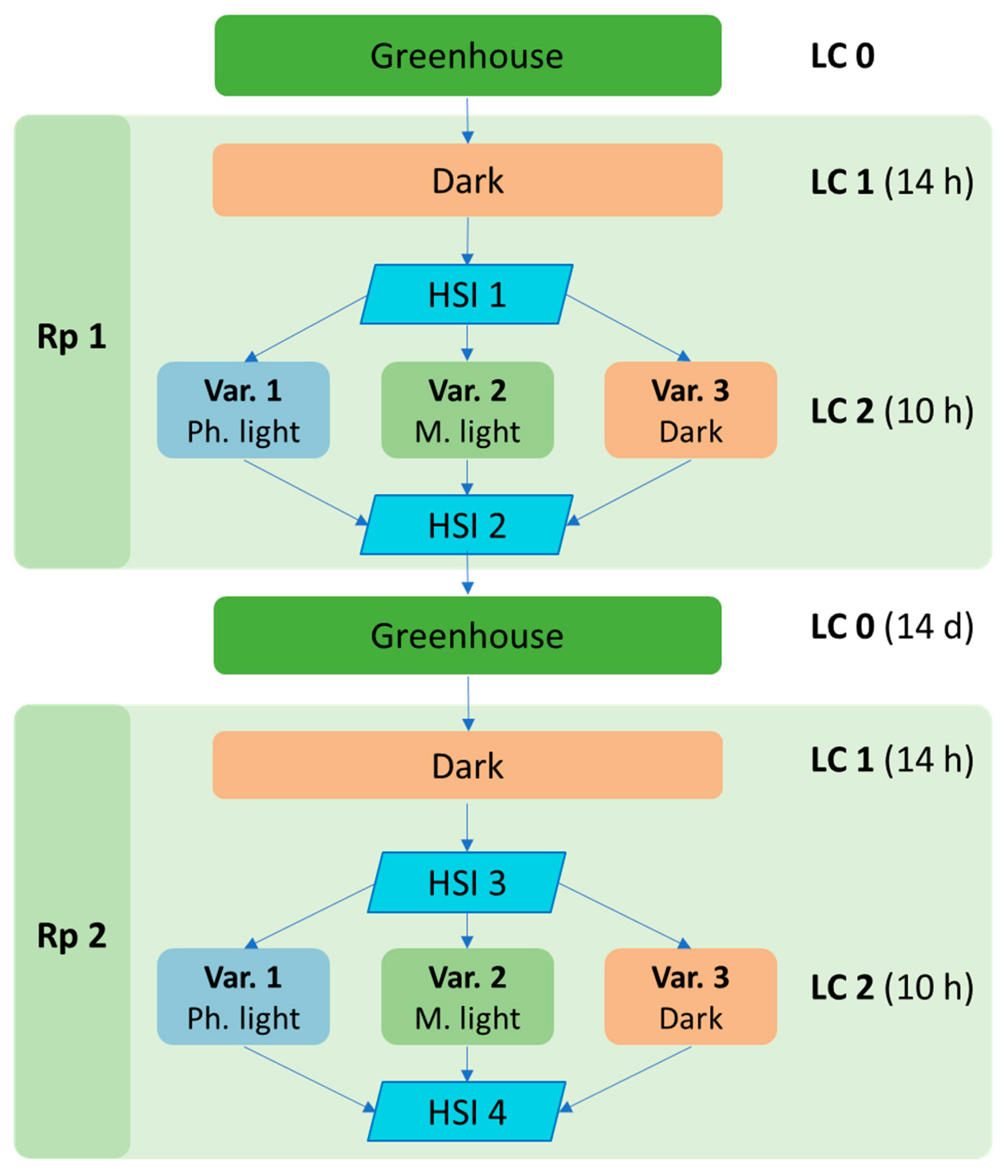
Nine genetically homogeneous Ficus elastica plants, which were previously kept in the greenhouse conditions under natural light (Light conditions 0—LC 0), were placed in darkness for 14 h (LC 1). After exposure to LC 1, three plants were placed at a distance of 40 cm from the leaf under photoinhibitory light (Variant 1—Var. 1, LC 2, light stress) having a photosynthetic photon flux density (PPFD) of 200 µmol photons m−2 s−1. Three plants were placed under moderate light (Var. 2, LC 2, shade) (PPFD = 50 µmol photons m−2 s−1), and the remaining three plants were returned to the dark (Var. 3, LC 2). The levels of PPFD were measured using a PAR sensor of a Waltz Diving-PAM fluorometer. The duration of exposure at LC 2 was 10 h. After the experiment (Repetition 1—Rp 1), the plants were returned to the greenhouse. Two weeks later, the experiment was repeated (Rp 2). HSI was performed 4 times (HSI 1–HSI 4), before and after LC 2.
The third ficus leaf from the top was always used to obtain the hyperspectral data. The block diagram of the experiment is shown in
Figure 3.
After HSI data preprocessing, 30 to 40 spectral profiles were randomly selected for each leaf from the top of the leaf blade since it is the flattest area which causes minimal distortion compared with the bottom and middle parts of the leaf blade. These bottom and middle parts are strongly curved symmetrically to the central vein.
The t-test and random forest (RF) were used to identify spectral ranges that allow for diagnosing light stress in plants. The choice of significant spectral ranges was carried out according to the values of the significance level of the t-test, out-of-bag (OOB) estimate of the error rate, mean decrease accuracy, and mean decrease Gini according to the results of RF pixel-based classification.
The experimentally calculated light stress index (LSI), was tested with RF against 125 spectral bands (SB) and 80 vegetation indices (VIs) for the mean decrease Gini and the mean decrease accuracy.
Statistical and mathematical analyses of the obtained results were carried out using the R environment [
27].
Detailed information on these 80 VIs can be found in the work of Dmitriev et al. [
28].
3. Results
3.1. Selection of the Most Informative SB for Identification of Light Stress
3.1.1. Selecting SB Using t-Test
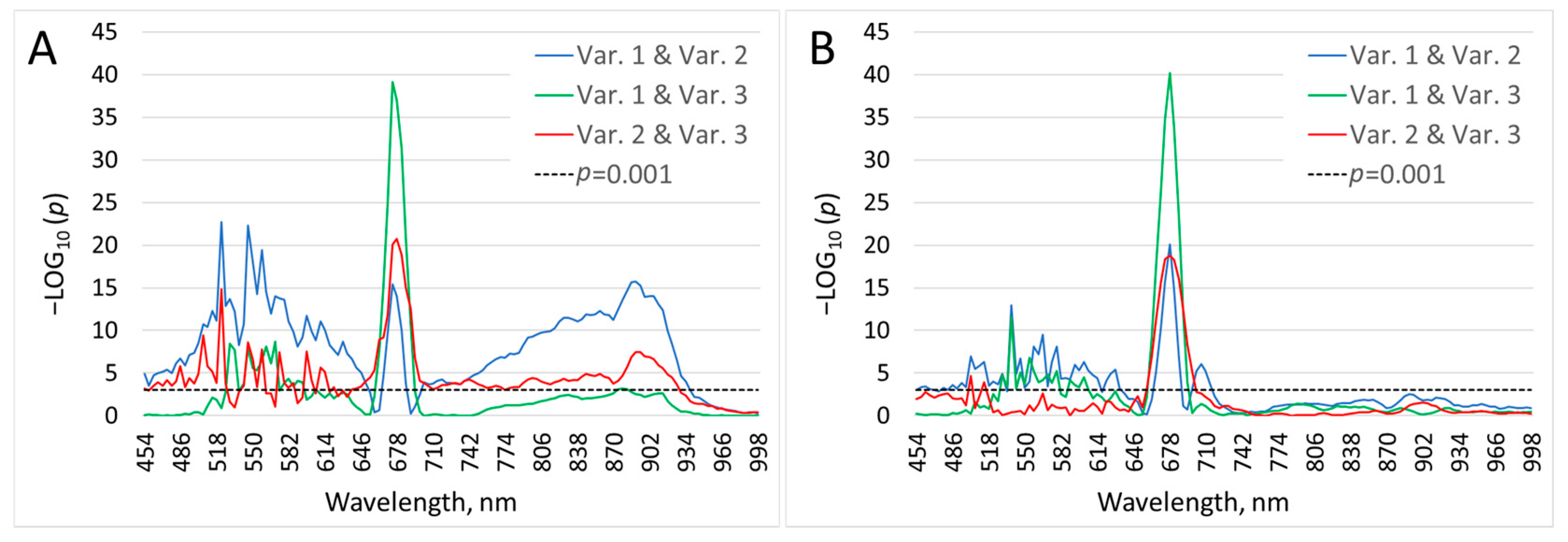
To select the most informative spectral ranges, the values of the SB of the same ranges were compared between different lighting conditions (LC 2) using a
t-test. The comparison results are presented in
Supplementary Table S1 and
Figure 4. For some compared bands, the level of significance (
p) is lower than 0.0001. This did not allow for representing the dynamics of the significance level visually and proportionally in the form of a curve in the figure imposed over the entire spectrum. Therefore, the significance level values were converted to the negative decimal logarithm (–log
10p). The dynamics of –log
10p over SB are shown in
Figure 4.
The first zone in which significant differences are observed according to the variants in both repetitions of the experiment lies in the range of 498–610 nm. The peak of significance of the difference between the variants, in terms of the values of the SB, falls at 680–690 nm, i.e., the zone of chlorophyll fluorescence.
3.1.2. Selection of SBs by Their Contribution to Mean Decrease Accuracy and Mean Decrease Gini Based on the Results of RF Pixel-Based Classification
Next, the RF classification was used to select spectral ranges. It was applied to classify spectral profiles belonging to different lighting conditions (LC 2).
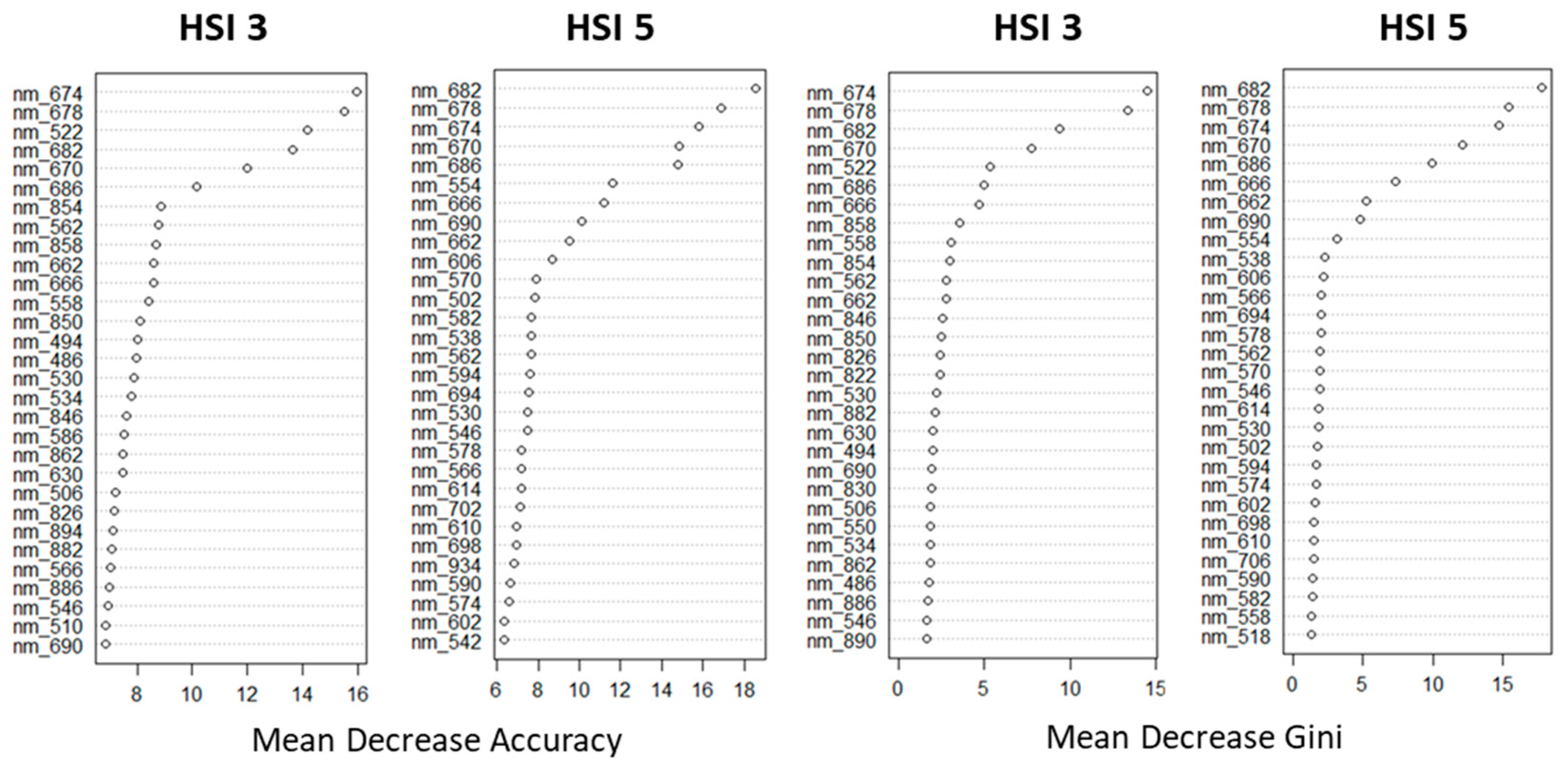
The SBs that have the greatest impact on Mean Decrease Accuracy and Mean Decrease Gini are shown in
Figure 5.
Summarizing the results, the most important SB for mean decrease accuracy and mean decrease Gini for the two repetitions of the experiment lie in the ranges of 662–690 nm and 522–554 nm. Thus, in the process of identifying different lighting conditions, the RF pixel-based classification method revealed a significant effect of chlorophyll fluorescence in the red zone of the spectrum.
3.1.3. Selection of SBs by Searching for Their Optimal Combinations for RF Pixel-Based Classification
Spectral bands were selected according to their contribution to the OOB estimate of the error rate. A simple selection algorithm has been chosen that does not require significant computing resources. First, the pair of SBs that produced the smallest OOB estimate of the error rate was selected. Next, a third band was selected for this SB pair, which, in combination with the first pair, gave the lowest error, and so on. The number of combinations of SBs (Y) is determined by the following equation:
where n—number of bands.
The comparison was carried out for all pairs of variants (Var. 1 and Var. 2; Var. 1 and Var. 3; Var. 2 and Var. 3;) under different light conditions (LC 2) for HSI 3 and HSI 5. Spectral bands were ranked by their contribution to the OOB estimate of the error rate (
Supplementary Table S2). Based on the pairs of SBs that make the greatest contribution to the decrease in the OOB estimate of the error rate, two spectral ranges were determined: 522–594 nm and 666–682 nm (
Figure 6).
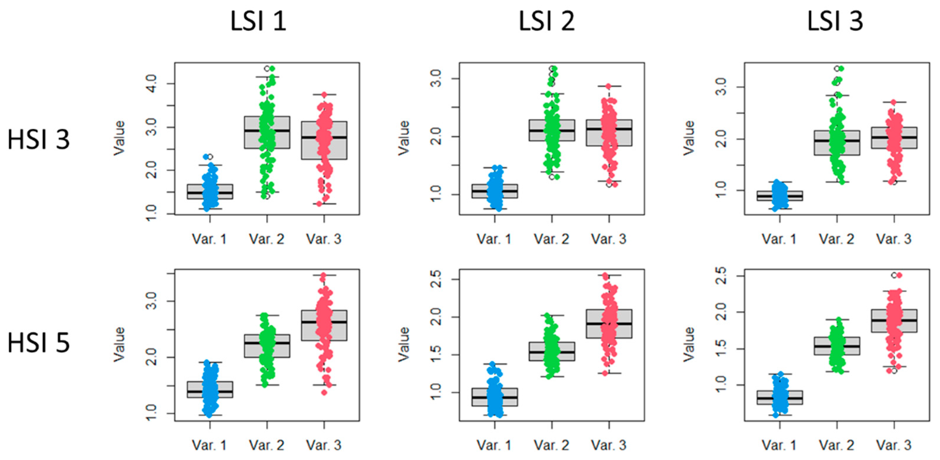
3.2. Comparison of a Simple Ratio of the Detected Spectral Ranges for the Identification of Light Stress
Three variants of significant spectral ranges were selected:
using a t-test (682–690 nm and 498–610 nm);
by the contribution of SBs to the mean decrease accuracy and the mean decrease Gini according to the results of RF pixel-based classification (662–690 nm and 522–554 nm);
by selecting the optimal combinations of SBs according to the value of the OOB estimate of the error rate of RF pixel-based classification (666–682 nm and 522–594 nm).
Further, based on the spectral ranges established for the identification of light stress, their simple ratios were calculated and tested.
A comparison of boxplots of three variants (Var.1, Var.2, and Var.3) based on the results of HSI 3 and HSI 5 allows us to make a preliminary conclusion that LSI 3 is more informative for detecting light stress than LSI 1 and LSI 2 (
Figure 7).
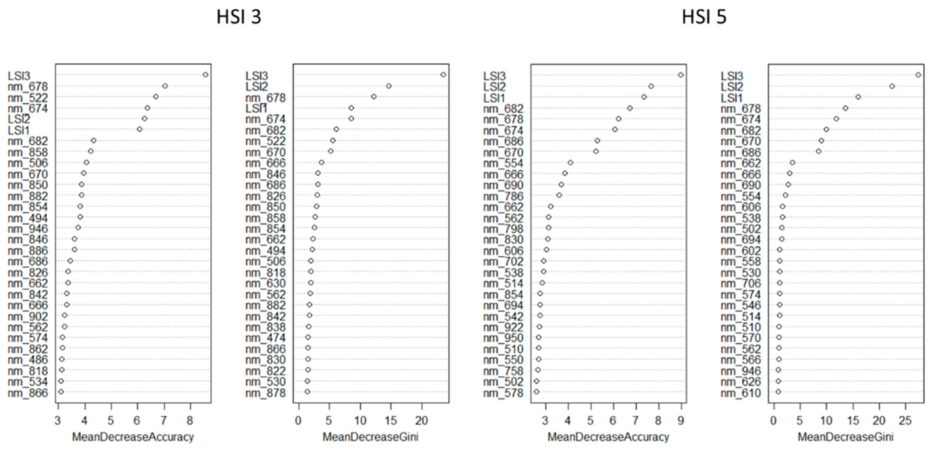
3.2.1. Comparison of LSI 1, LSI 2, and LSI 3 with SBs for the Identification of Light Stress
Classification of the state of ficus plants was carried out using RF pixel-based classification, according to values of the SB and LSI 1, LSI 2, and LSI 3. According to the classification results, LSI 3 has the largest contribution to the mean decrease accuracy and the mean decrease Gini values (
Figure 8).
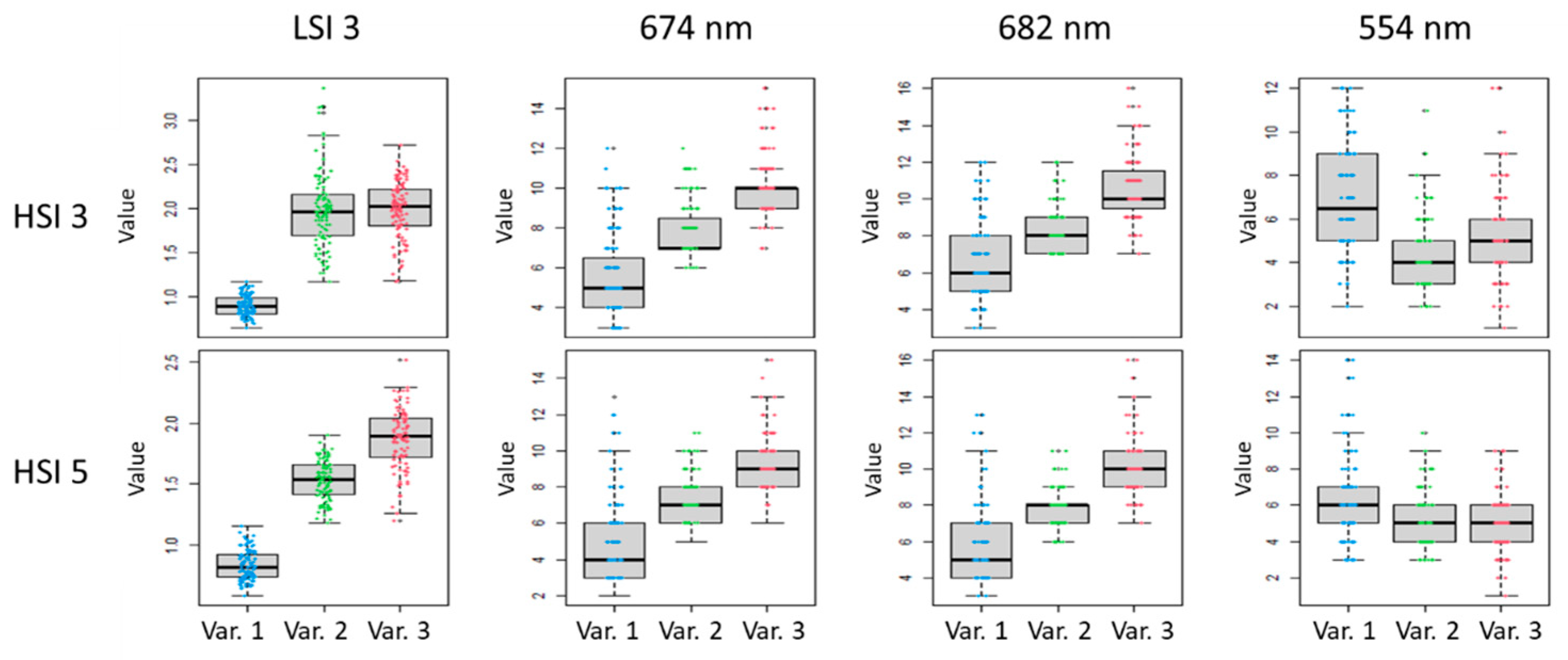
Boxplots of the LSI 3 values of three LC 2 variants (Var. 1, Var. 2, and Var. 3), according to the results of HSI 3 and HSI 5, compared to values of the SB 674 nm, 682 nm and 554 nm, are shown in
Figure 9.
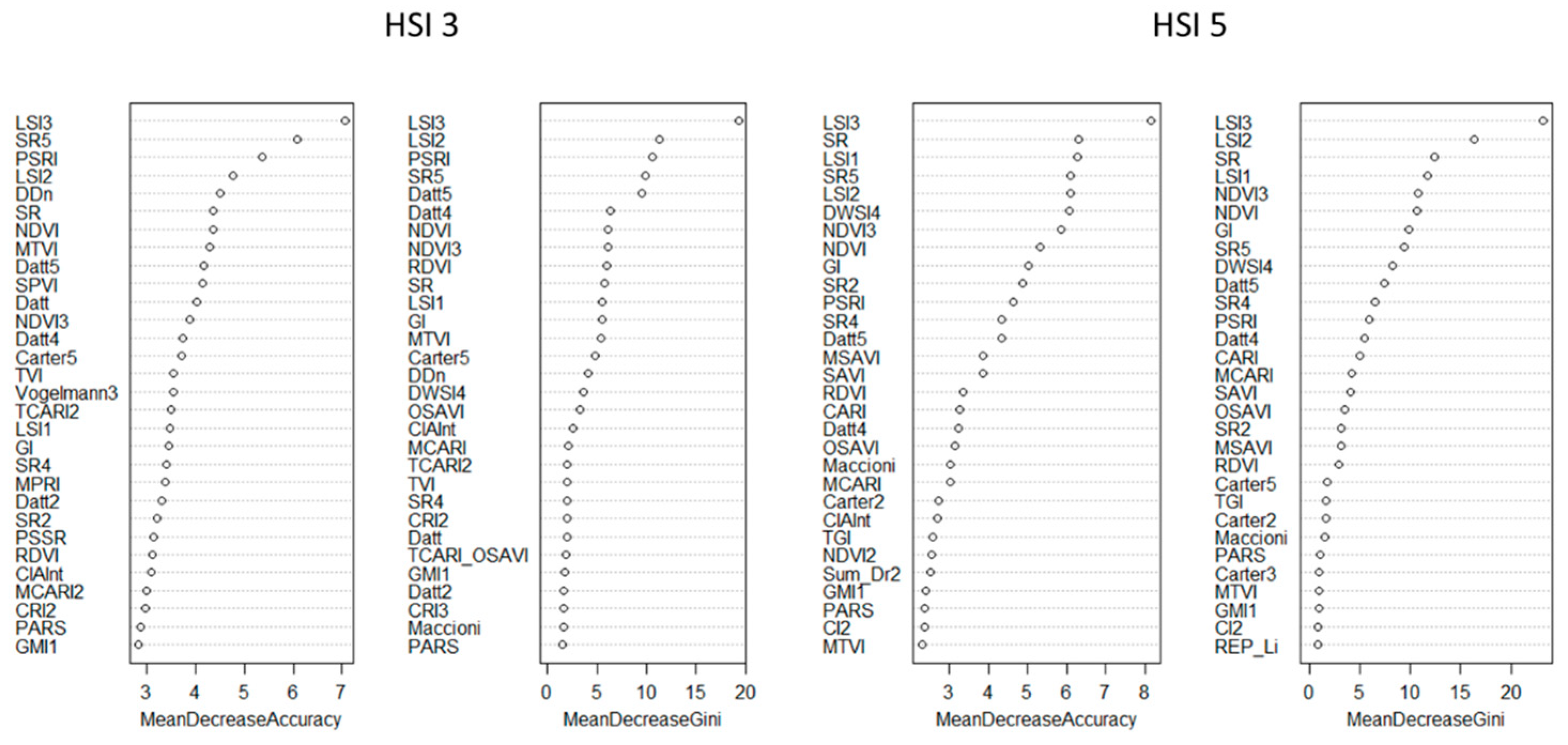
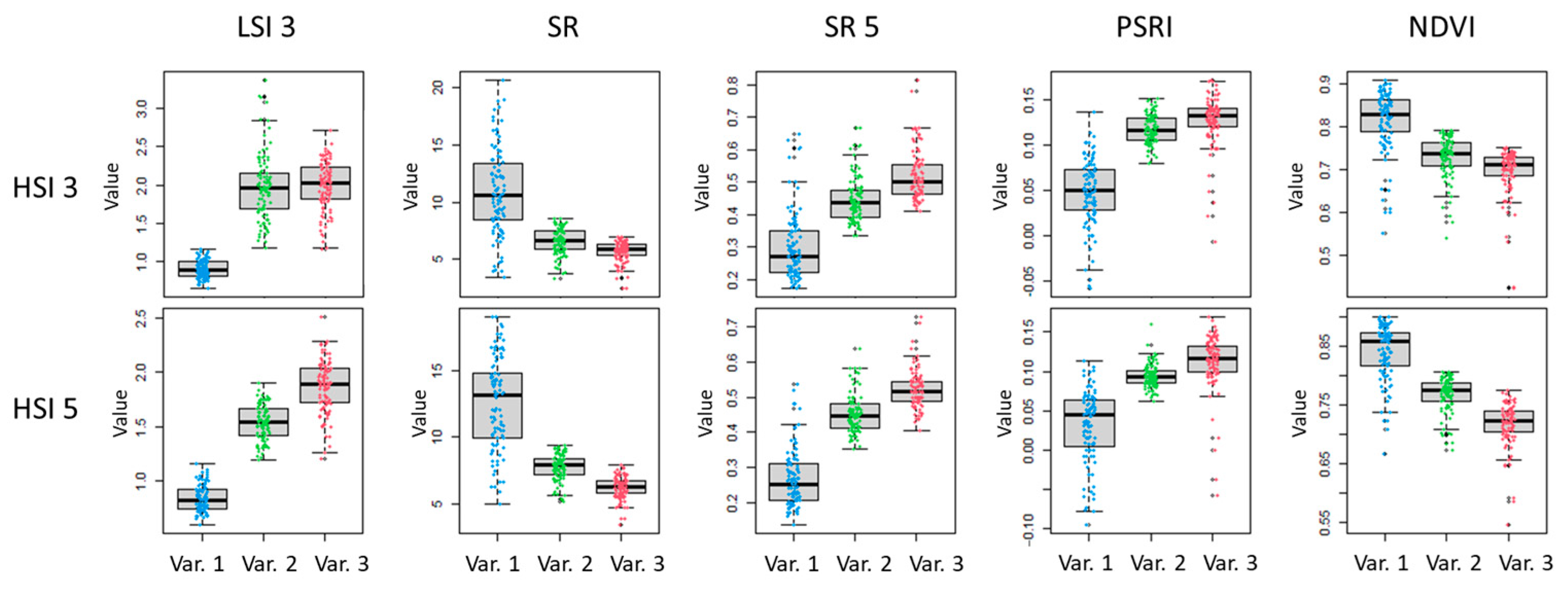
3.2.2. Comparison of LSI 1, LSI 2, and LSI 3 with VIs for the Identification of Light Stress
When testing LSI 1, LSI 2, and LSI 3 values with 80 VIs using RF pixel-based classification, LSI 3 turned out to be the most significant depending on the mean decrease accuracy and the mean decrease Gini, as in the case of comparison with SB (
Figure 10).
Boxplots of the LSI 3 values of three LC 2 variants (Var. 1, Var. 2, and Var. 3), based on the results of HSI 3 and HSI 5 compared to the values of VIs SR, SR5, PSRI and NDVI, are presented in
Figure 11.
3.3. Light-Stress Index (LSI)
The LSI 3 values of the three LC 2 variants (Var. 1, Var. 2, and Var. 3), obtained according to the results of HSI 3 and HSI 5, were distributed under a normal law (
Figure 12). This allows for the use of both parametric and nonparametric methods of statistical analysis when working with LSI 3.
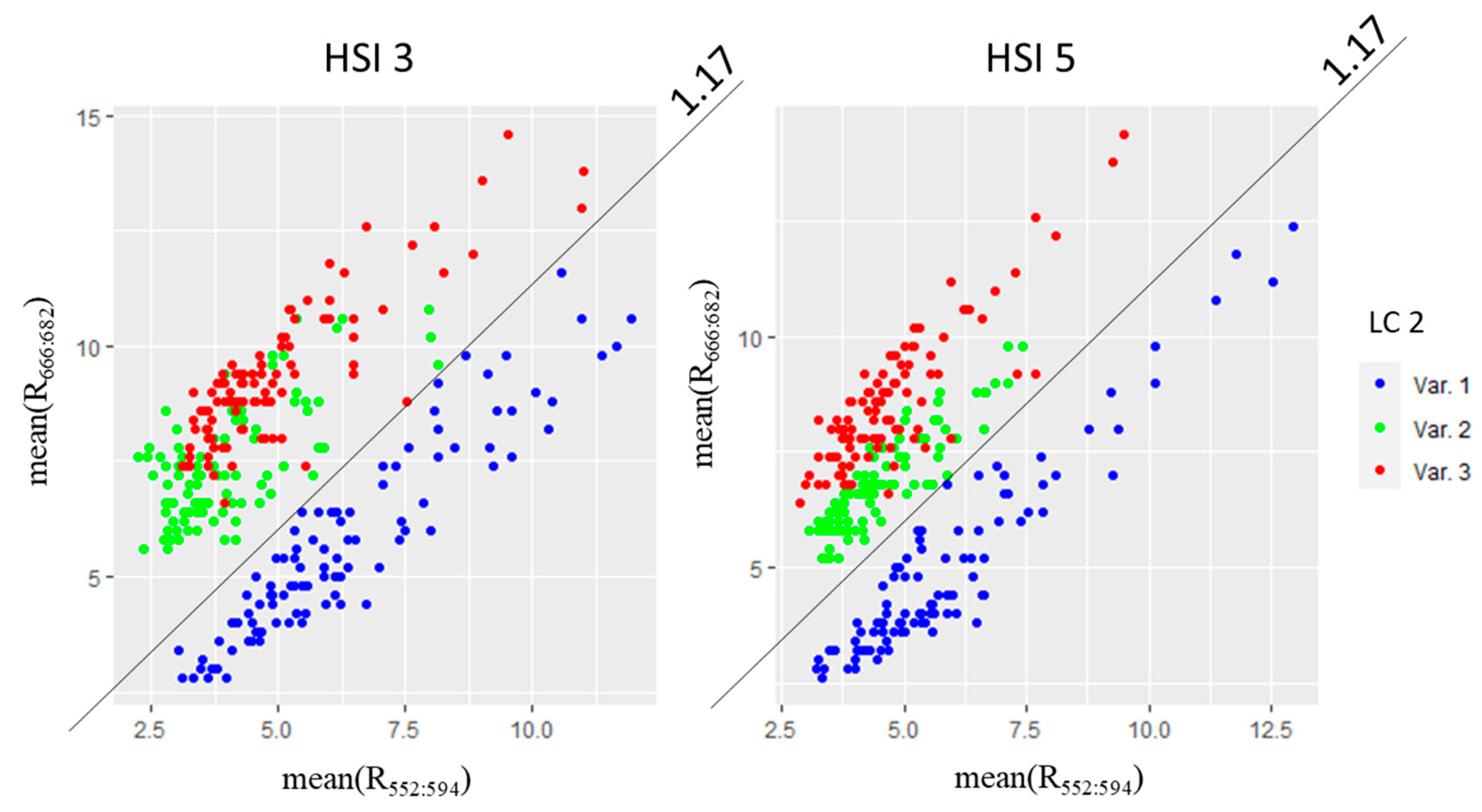
It has been found that there is a linear relationship between the average values of the spectral ranges 666–682 nm and 522–594 nm (
Figure 13). Therefore, a specific range of LSI 3 values may be applied to identify and evaluate the magnitude of light stress. It was preliminarily found that the LSI 3 threshold, which separates light stress from other plant states, is 1.17. Additional studies are needed to develop and verify the LSI 3 scale, which would allow for the light history of plants to be considered.
4. Discussion
Light stress [
29,
30,
31], just like other types of stress [
10,
11,
12,
13,
14], is known to be accompanied by a decrease in chlorophyll, which has two absorption maxima in the blue and red bands. On this basis, one would expect that, in response to light, the most pronounced changes in the reflectance spectra of the leaves would be an increase in the reflectance in these bands and possibly a slight increase in the reflectance in the green band. In addition, the far-red light range (680–740 nm) which corresponds to the chlorophyll fluorescence emission may be a stress-sensitive area, considering that it is inversely dependent on the photosynthesis rate [
32]. However, studies have shown that light stress resulted in an increase in reflection in the yellow–green range and a decrease in reflection in the red range. In addition, the
t-test and RF methods used in the experiments allowed for the of revealing three pairs of the most relevant ranges for light stress. They are 682–690 nm and 498–610 nm; 662–690 nm and 522–554 nm; and 666–682 nm and 522–594 nm. These ranges do not coincide with the sensitive ranges known for other types of stress. Thus, Navarro et al. [
33] showed that ranges 492–504 and 540–568 nm of visible light; 712–720 nm of far-red light; and 855, 900–908, and 970 nm of near-infrared light had the best sensitivity to pathogen-induced stress occurring in
Diplotaxis tenuifolia plants. In several studies, other reflectance spectral ranges indicative of different types of stress (not related to photoinhibition) have been proposed, 850, 630, 535, and 465 nm [
15]; 500–660 nm [
34]; and 690 and 702 nm [
9].
Light stress and light history had the most influence on the SB 690–700 nm and 730–750 nm [
35], which is not consistent, but also not contradictory, with our data. The use of the three light-stress-sensitive ranges identified in our work makes it possible to increase the sensitivity and reliability of the indication of this type of stress.
The causes of the detected stress-induced increase in reflectance in the yellow–green range and the drop in reflectance in the red range are not clear. Possible reasons for this could be:
Changes in pigment concentrations—decrease in carotenoids, which absorb well in the yellow–green range and do not absorb in the red range and increase in chlorophyll a, which, being a component of light-harvesting complexes (LHC) 1 and LHC 2, absorbs well in the 666–682 nm range, but does not absorb in the yellow-green range [
36];
Light-induced rearrangements of chloroplast localization, which can lead to shifts in light absorption by the pigments without changing their concentration [
37].
However, irrespective of their cause (which is beyond the scope of this study), the observed shifts can serve as indicators of light stress and can be taken into account when calculating VIs. The light-stress index (LSI = mean(R
666:682)/mean(R
522:594) calculated on the basis of these ranges appeared to be the most sensitive to light stress compared to the SB and 80 VIs [
28] selected for testing. If it is possible to develop and verify a scale for LSI, it would be possible to significantly simplify the identification of light stress.
In addition, the results of the study confirm the need for remote spectral monitoring of vegetation, taking into account its light history, which was previously pointed out by other authors [
38,
39,
40,
41].
In general, it can be said that the combination of the technical capabilities of a hyperspectral camera, with the method of machine learning [
8,
42,
43] in the processing of hyperspectral data, opens up great prospects for the early diagnosis of plant stress.
5. Conclusions
The study performed in this work showed that the previous history of the illumination of leaves has a significant impact on their spectral characteristics. It has been established that two spectral ranges are significant for the identification of light stress. Intense artificial lighting leads to an increase in reflection in the range of 552–594 nm and a decrease in reflection in the range of 666–682 nm. Based on empirical data, the light stress index (LSI) = mean(R666:682)/mean(R552:594) was calculated and tested. LSI allows more accurate identification of the state of light stress compared to the SB and 80 VIs tested in the study. The LSI values are distributed according to the normal law, which makes it possible to use parametric statistics when working with it. It has been preliminarily established that the LSI threshold separating light stress from the normal state of the plant is 1.17. The results obtained indicate the possibility of identifying light stress in plants using spectral sensors that detect passive reflection. In addition, the results of the study confirm the need to take into account the light history in the remote spectral monitoring of vegetation.
The result of the study was reproduced in time in two repetitions. If this result is confirmed on other plant objects, then this may be of practical importance for monitoring the light stress of plants by means of remote sensing.
Author Contributions
Conceptualization, P.A.D., B.L.K. and V.S.L.; Data curation, B.L.K. and A.A.D.; Formal analysis, A.A.D.; Investigation, P.A.D. and A.A.D.; Methodology, P.A.D.; Project administration, P.A.D.; Resources, V.A.C. and T.V.V.; Software, A.A.D.; Writing—original draft, P.A.D. and B.L.K.; Writing—review and editing, P.A.D., B.L.K. and V.S.L. All authors have read and agreed to the published version of the manuscript.
Funding
The project was supported by the Russian Science Foundation under grant No. 22-14-00338,
https://rscf.ru/project/22-14-00338/ (accessed on 1 September 2023), and performed at Southern Federal University (Rostov-on-Don, Russian Federation).
Data Availability Statement
Conflicts of Interest
The authors declare no conflict of interest.
References
- Suzuki, N.; Devireddy, A.R.; Inupakutika, M.A.; Baxter, A.; Miller, G.; Song, L.; Shulaev, E.; Azad, R.K.; Shulaev, V.; Mittler, R. Ultra-fast alterations in mRNA levels uncover multiple players in light stress acclimation in plants. Plant J. 2015, 84, 760–772. [Google Scholar] [CrossRef] [PubMed]
- Ruban, A.V. Evolution under the sun: Optimizing light harvesting in photosynthesis. J. Exp. Bot. 2015, 66, 7–23. [Google Scholar] [CrossRef] [PubMed]
- Murata, N.; Takahashi, S.; Nishiyama, Y.; Allakhverdiev, S.I. Photoinhibition of photosystem II under environmental stress. Biochim. Biophys. Acta 2007, 1767, 414–421. [Google Scholar] [CrossRef] [PubMed]
- Balfagón, D.; Sengupta, S.; Gómez-Cadenas, A.; Fritschi, F.B.; Azad, R.K.; Mittler, R.; Zandalinas, S.I. Jasmonic Acid Is Required for Plant Acclimation to a Combination of High Light and Heat Stress. Plant Physiol. 2019, 181, 1668–1682. [Google Scholar] [CrossRef] [PubMed]
- Grieco, M.; Roustan, V.; Dermendjiev, G.; Rantala, S.; Jain, A.; Leonardelli, M.; Neumann, K.; Berger, V.; Engelmeier, D.; Bachmann, G.; et al. Adjustment of photosynthetic activity to drought and fluctuating light in wheat. Plant Cell Environ. 2020, 43, 1484–1500. [Google Scholar] [CrossRef] [PubMed]
- Mishanin, V.I.; Trubitsin, B.V.; Patsaeva, S.V.; Ptushenko, V.V.; Solovchenko, A.E.; Tikhonov, A.N. Acclimation of shade-tolerant and light-resistant Tradescantia species to growth light: Chlorophyll a fluorescence, electron transport, and xanthophyll content. Photosynth. Res. 2017, 133, 87–102. [Google Scholar] [CrossRef] [PubMed]
- Kureel, N.; Sarup, J.; Matin, S.; Goswami, S.; Kureel, K. Modelling vegetation health and stress using hypersepctral remote sensing data. Model. Earth Syst. Environ. 2022, 8, 733–748. [Google Scholar] [CrossRef]
- Duarte-Carvajalino, J.M.; Silva-Arero, E.A.; Góez-Vinasco, G.A.; orres-Delgado, L.M.; Ocampo-Paez, O.D.; Castaño-Marín, A.M. Estimation of Water Stress in Potato Plants Using Hyperspectral Imagery and Machine Learning Algorithms. Horti-Culturae 2021, 7, 176. [Google Scholar] [CrossRef]
- Qin, J.; Monje, O.; Nugent, M.R.; Finn, J.R.; O’rourke, A.E.; Fritsche, R.F.; Baek, I.; Chan, D.E.; Kim, M.S. Development of a hyperspectral imaging system for plant health monitoring in space crop production. In Proceedings of the SPIE 12120, Sensing for Agriculture and Food Quality and Safety XIV, Orlando, FL, USA, 1 June 2022; Volume 1212004. [Google Scholar] [CrossRef]
- Faqeerzada, M.A.; Park, E.; Kim, T.; Kim, M.S.; Baek, I.; Joshi, R.; Kim, J.; Cho, B.-K. Fluorescence Hyperspectral Imaging for Early Diagnosis of Heat-Stressed Ginseng Plants. Appl. Sci. 2023, 13, 31. [Google Scholar] [CrossRef]
- Burnett, A.C.; Serbin, S.P.; Davidson, K.J.; Ely, K.S.; Rogers, A. Detection of the metabolic response to drought stress using hyperspectral reflectance. J. Exp. Bot. 2021, 72, 6474–6489. [Google Scholar] [CrossRef]
- Bahe, M.M.; Murphy, R.L.; Russell, M.B.; Knight, J.F.; Johnson, G.R. Suitability of a single imager multispectral sensor for tree health analysis. Urban For. Urban Green. 2021, 63, 1618–8667. [Google Scholar] [CrossRef]
- Xie, C.; Yang, C.; Moghimi, A. Detection of cold stressed maize seedlings for high throughput phenotyping using hyperspectral imagery. In Proceedings of the SPIE 10213, Hyperspectral Imaging Sensors: Innovative Applications and Sensor Standards, Anaheim, CA, USA, 28 April 2017; Volume 1021305. [Google Scholar] [CrossRef]
- Cotrozzi, L.; Couture, J.J. Hyperspectral assessment of plant responses to multi-stress environments: Prospects for managing protected agrosystems. Plants People Planet 2020, 2, 244–258. [Google Scholar] [CrossRef]
- Kitić, G.; Tagarakis, A.; Cselyuszka, N.; Panić, M.; Birgermajer, S.; Sakulski, D.; Matović, J. A new low-cost portable multi-spectral optical device for precise plant status assessment. Comput. Electron. Agric. 2019, 162, 300–308. [Google Scholar] [CrossRef]
- Lichtenthaler, H.K. Vegetation stress: An introduction to the stress concept in plants. J. Plant Physiol. 1996, 148, 4–14. [Google Scholar] [CrossRef]
- le Maire, G.; François, C.; Dufrêne, E. Towards universal broad leaf chlorophyll indices using PROSPECT simulated database and hyperspectral reflectance measurements. Remote Sens. Environ. 2004, 89, 1–28. [Google Scholar] [CrossRef]
- Wang, J.; Wu, W.; Wang, T.; Cai, C. Estimation of leaf chlorophyll content and density in Populus euphratica based on hyperspectral characteristic variables. Spectrosc. Lett. 2018, 51, 485–495. [Google Scholar] [CrossRef]
- Wang, J.; Yin, C.; Wang, T.; Zhai, Y.; Cai, C. Seasonal Variation Characteristics of Chlorophyll and Spectrum in Leaves of Populus eu-phratica Under Water Stress. J. Appl. Spectrosc. 2021, 88, 622–632. [Google Scholar] [CrossRef]
- Bondarava, N.; Gross, C.M.; Mubarakshina, M.; Golecki, J.R.; Johnson, G.N.; Krieger-Liszkay, A. Putative function of cyto-chrome b559 as a plastoquinol oxidase. Physiol. Plant. 2010, 138, 463–473. [Google Scholar] [CrossRef]
- Zulfugarov, I.S.; Tovuu, A.; Eu, Y.J.; Dogsom, B.; Poudyal, R.S.; Nath, K.; Hall, M.; Banerjee, M.; Yoon, U.C.; Moon, Y.H.; et al. Production of superoxide from Photosystem II in a rice (Oryza sativa L.) mutant lacking PsbS. BMC Plant Biol. 2014, 14, 242. [Google Scholar] [CrossRef]
- Takagi, D.; Takumi, S.; Hashiguchi, M.; Sejima, T.; Miyake, C. Superoxide and singlet oxygen produced within the thylakoid membranes both cause photosystem I photoinhibition. Plant Physiol. 2016, 171, 1626–1634. [Google Scholar] [CrossRef]
- Lingvay, M.; Akhtar, P.; Sebők-Nagy, K.; Páli, T.; Lambrev, P.H. Photobleaching of chlorophyll in light-harvesting complex II increases in lipid environment. Front. Plant Sci. 2020, 11, 849. [Google Scholar] [CrossRef] [PubMed]
- Strizh, K.; Neverov, V. Photoinhibition of photosystem II in vitro: Spectral and kinetic analyses. Russ. J. Plant Physiol. 2007, 54, 439–449. [Google Scholar] [CrossRef]
- Bareth, G.; Aasen, H.; Bendig, J.; Gnyp, M.L.; Bolten, A.; Jung, A.; Michels, R.; Soukkamaki, J. Low-weight and UAV-based hyperspectral full-frame cameras for monitoring crops: Spectral comparison with portable spectroradiometer measurements. Photogramm. Fernerkund. Geoinf. 2015, 1, 69–79. [Google Scholar] [CrossRef]
- Aasen, H.; Burkart, A.; Bolten, A.; Bareth, G. Generating 3D hyperspectral in-formation with lightweight UAV snapshot cameras for vegetation monitoring: From camera calibration to quality assurance. JPRS 2015, 108, 245–259. [Google Scholar] [CrossRef]
- R Core Team. R: A Language and Environment for Statistical Computing; R Foundation for Statistical Computing: Vienna, Austria, 2022; Available online: https://www.R-project.org/ (accessed on 1 September 2023).
- Dmitriev, P.A.; Kozlovsky, B.L.; Kupriushkin, D.P.; Dmitrieva, A.A.; Rajput, V.D.; Chokheli, V.A.; Tarik, E.P.; Kapralova, O.A.; Tokhtar, V.K.; Minkina, T.M.; et al. Assessment of Invasive and Weed Species by Hyperspectral Imagery in Agro-cenoses Ecosystem. Remote Sens. 2022, 14, 2442. [Google Scholar] [CrossRef]
- Zhou, R.; Yu, X.; Li, X.; dos Santos, T.M.; Rosenqvist, E.; Ottosen, C.-O. Combined high light and heat stress induced complex response in tomato with better leaf cooling after heat priming. Plant Physiol. Biochem. 2020, 151, 1–9. [Google Scholar] [CrossRef] [PubMed]
- Agathokleous, E.; Feng, Z.Z.; Peñuelas, J. Chlorophyll hormesis: Are chlorophylls major components of stress biology in higher plants? Sci. Total Environ. 2020, 726, 138637. [Google Scholar] [CrossRef]
- Mendoza, F.; Berry, C.; Prestigiacomo, L.; Van Hoewyk, D. Proteasome inhibition rapidly exacerbates photoinhibition and impedes recovery during high light stress in Chlamydomonas reinhardtii. BMC Plant Biol. 2020, 20, 22. [Google Scholar] [CrossRef]
- Lysenko, V.; Rajput, V.D.; Kumar Singh, R.; Guo, Y.; Kosolapov, A.; Usova, E.; Varduny, T.; Chalenko, E.; Yadronova, O.; Dmitriev, P.; et al. Chlorophyll fluorometry in evaluating photosynthetic performance: Key limitations, possibilities, perspectives and alternatives. Physiol. Mol. Biol. Plants 2022, 28, 2041–2056. [Google Scholar] [CrossRef]
- Navarro, A.; Nicastro, N.; Costa, C.; Pentangelo, A.; Cardarelli, M.; Ortenzi, L.; Pallottino, F.; Cardi, T.; Pane, C. Sorting biotic and abiotic stresses on wild rocket by leaf-image hyperspectral data mining with an artificial intelligence model. Plant Methods 2022, 18, 45. [Google Scholar] [CrossRef]
- Wang, S.; Zhang, X.; Ma, Y.; Li, X.; Cheng, M.; Zhang, X.; Liu, L. Detecting Sulfuric and Nitric Acid Rain Stresses on Quercus glauca through Hyperspectral Responses. Sensors 2018, 18, 830. [Google Scholar] [CrossRef] [PubMed]
- Zarco-Tejada, P.J.; Miller, J.R.; Mohammed, G.H.; Noland, T.L.; Sampson, P.H. Estimation of chlorophyll fluorescence under natural illumination from hyperspectral data. Int. J. Appl. Earth Obs. Geoinf. 2001, 3, 321–327. [Google Scholar] [CrossRef]
- Laisk, A.; Oja, V.; Eichelmann, H.; Dall’Osto, L. Action spectra of photosystems II and I and quantum yield of photo-synthesis in leaves in State 1. Biochim. Biophys. Acta 2014, 1837, 315–325. [Google Scholar] [CrossRef] [PubMed]
- Baránková, B.; Lazár, D.; Nauš, J. Analysis of the effect of chloroplast arrangement on optical properties of green tobacco leaves. Remote Sens. Environ. 2016, 174, 181–196. [Google Scholar] [CrossRef]
- Kohzuma, K.; Tamaki, M.; Hikosaka, K. Corrected photochemical reflectance index (PRI) is an effective tool for detecting environmental stresses in agricultural crops under light conditions. J. Plant Res. 2021, 134, 683–694. [Google Scholar] [CrossRef] [PubMed]
- Atherton, J.; Olascoaga, B.; Alonso, L.; Porcar-Castell, A. Spatial variation of leaf optical properties in a boreal forest is influenced by species and light environment. Front. Plant Sci. 2017, 8, 309. [Google Scholar] [CrossRef] [PubMed]
- Gamon, J.A.; Berry, J.A. Facultative and constitutive pigment effects on the Photochemical eflectance Index (PRI) in sun and shade conifer needles. Isr. J. Plant Sci. 2012, 60, 85–95. [Google Scholar] [CrossRef]
- Schmiege, S.C.; Griffin, K.L.; Boelman, N.T.; Vierling, L.A.; Bruner, S.G.; Min, E.; Maguire, A.J.; Jensen, J.; Eitel, J.U.H. Vertical gradients in photosynthetic physiology diverge at the latitudinal range extremes of white spruce. Plant Cell Environ. 2022, 46, 45–63. [Google Scholar] [CrossRef]
- Sonobe, R.; Hirono, Y.; Oi, A. Non-Destructive Detection of Tea Leaf Chlorophyll Content Using Hyperspectral Reflectance and Machine Learning Algorithms. Plants 2020, 9, 368. [Google Scholar] [CrossRef]
- Zubler, A.V.; Yoon, J.-Y. Proximal Methods for Plant Stress Detection Using Optical Sensors and Machine Learning. Biosensors 2020, 10, 193. [Google Scholar] [CrossRef]
Figure 1.
Hyperspectral imaging of F. elastica leaves. (A) Cubert UHD-185; (B) object of study; (C) artificial light sources for HSI.
Figure 1.
Hyperspectral imaging of F. elastica leaves. (A) Cubert UHD-185; (B) object of study; (C) artificial light sources for HSI.
Figure 2.
Integral spectrum of artificial light sources reflected from a white standard. Measured with a Cubert UHD 185 camera with a 4 nm step.
Figure 2.
Integral spectrum of artificial light sources reflected from a white standard. Measured with a Cubert UHD 185 camera with a 4 nm step.
Figure 3.
Block diagram of an experiment to study shifts in the spectral reflection characteristics of F. elastica leaves in the range of 450–950 nm. Var 1, light stress—10 h exposure to the photoinhibitory light (200 µmol photons m−2 s−1); Var. 2, shade—moderate light (50 µmol photons m−2 s−1); Var 3—dark-adapted plants. HSI 1–4—plant HSI; LC 0–2—light conditions; Rp 1–2—repetition of the experiment.
Figure 4.
The −log10p values, depending on the SB, when comparing variants (Var. 1, Var. 2, Var. 3; LC 2) by pairs. (A)—t-test (HSI 3); (B)—t-test (HSI 5).
Figure 4.
The −log10p values, depending on the SB, when comparing variants (Var. 1, Var. 2, Var. 3; LC 2) by pairs. (A)—t-test (HSI 3); (B)—t-test (HSI 5).
Figure 5.
Ranking SBs by their contribution to mean decrease accuracy and mean decrease Gini.
Figure 5.
Ranking SBs by their contribution to mean decrease accuracy and mean decrease Gini.
Figure 6.
Pairs of SBs that make the greatest contribution to the decrease in the OOB estimate of the error rate.
Figure 6.
Pairs of SBs that make the greatest contribution to the decrease in the OOB estimate of the error rate.
Figure 7.
Boxplots of LSI 1, LSI 2, and LSI 3 values of three LC 2 variants (Var. 1, Var. 2, and Var. 3) based on the results of HSI 3 and HSI 5.
Figure 7.
Boxplots of LSI 1, LSI 2, and LSI 3 values of three LC 2 variants (Var. 1, Var. 2, and Var. 3) based on the results of HSI 3 and HSI 5.
Figure 8.
The most significant SB and LSI for indicating light stress in ficuses, depending on the mean decrease accuracy and the mean decrease Gini.
Figure 8.
The most significant SB and LSI for indicating light stress in ficuses, depending on the mean decrease accuracy and the mean decrease Gini.
Figure 9.
Boxplots of LSI 3 values compared to the values of the individual most significant SB.
Figure 9.
Boxplots of LSI 3 values compared to the values of the individual most significant SB.
Figure 10.
The most significant VIs for identifying ficus light stress, depending on the mean decrease accuracy and mean decrease Gini.
Figure 10.
The most significant VIs for identifying ficus light stress, depending on the mean decrease accuracy and mean decrease Gini.
Figure 11.
Boxplots of LSI 3 values compared to individual most significant VIs.
Figure 11.
Boxplots of LSI 3 values compared to individual most significant VIs.
Figure 12.
Distribution of the LSI 3 values of three LC 2 variants (Var. 1, Var. 2, and Var. 3) according to the results of HSI 3 and HSI 5 simultaneously.
Figure 12.
Distribution of the LSI 3 values of three LC 2 variants (Var. 1, Var. 2, and Var. 3) according to the results of HSI 3 and HSI 5 simultaneously.
Figure 13.
Distribution of mean(R666:682) against mean(R522:594) values of three variants (Var. 1, Var. 2, and Var. 3) for HSI 3 and HSI 5.
Figure 13.
Distribution of mean(R666:682) against mean(R522:594) values of three variants (Var. 1, Var. 2, and Var. 3) for HSI 3 and HSI 5.
| Disclaimer/Publisher’s Note: The statements, opinions and data contained in all publications are solely those of the individual author(s) and contributor(s) and not of MDPI and/or the editor(s). MDPI and/or the editor(s) disclaim responsibility for any injury to people or property resulting from any ideas, methods, instructions or products referred to in the content. |
© 2023 by the authors. Licensee MDPI, Basel, Switzerland. This article is an open access article distributed under the terms and conditions of the Creative Commons Attribution (CC BY) license (https://creativecommons.org/licenses/by/4.0/).


 ,
, 