Article

Soil Attributes Mapping with Online Near-Infrared Spectroscopy Requires Spatio-Temporal Local Calibrations

by
Ricardo Canal Filho
*,
José Paulo Molin
,
Marcelo Chan Fu Wei
and
Eudocio Rafael Otavio da Silva
Laboratory of Precision Agriculture (LAP), Department of Biosystems Engineering, “Luiz de Queiroz” College of Agriculture (ESALQ), University of Sao Paulo (USP), Piracicaba 13418-900, Brazil
*
Author to whom correspondence should be addressed.
AgriEngineering 2023, 5(3), 1163-1177; https://doi.org/10.3390/agriengineering5030074
Submission received: 10 March 2023 / Revised: 9 June 2023 / Accepted: 26 June 2023 / Published: 3 July 2023

Abstract

:
Building machine learning (ML) calibrations using near-infrared (NIR) soil spectroscopy direct in agricultural areas (online NIR), soil attributes can be fine-scale mapped in a faster and more cost-effective manner, guiding management decisions to ensure the maintenance of soil functions. However, a financially and environmentally unattractive density of 3–5 laboratory soil samples per ha is required to build these calibrations. Since no reports have evaluated if they are reusable or if a new calibration is required for each acquisition, this study’s objective was to acquire online NIR spectra in an agricultural field where ML models were previously built and validated, assessing their performance over time. Two spectral acquisitions were held over a fallow tropical field, separated by 21 days. Soil properties (clay, organic matter, cation exchange capacity, pH, phosphorus, potassium, calcium, and magnesium) were predicted using principal components regression models calibrated with day 1 spectra. Day 1 and day 21 predicted values and maps interpolated by ordinary kriging were compared. Spectra characteristics (morphology, features, and intensity) were evaluated. Predicted values from the two days were not correlated, as no causal relationship was found for the only Pearson’s correlation coefficient (r) significative at 99% (p < 0.01) (calcium, with r = 0.22 in the comparison pairing the nearest neighbors from the two days). For clay, organic matter, and cation exchange capacity, despite their robust prediction on day 1, no significative r values were found, ranging from −0.14 to 0.32, when comparing day 1 with day 21. The maps of the two days presented no similar spatial distribution, hindering their use for management decisions. Soil moisture is a suggested source of variation, but the analysis indicated that it was not the only one, requiring further investigation of the effect of soil surface conditions and environmental variables. Although further investigations should be performed, the results presented suggest that online NIR spectra ML models require spatio-temporal local calibrations to perform properly.

1. Introduction

In precision agriculture (PA), efforts are being made towards identifying spatial and temporal variability of agricultural systems to support management decisions aiming for efficient resource use, profitability, and sustainability of agricultural production [1]. The soil is essential to agriculture, providing water, nutrients, air, and mechanical sustentation for plants. Its intrinsic and extrinsic variability identification and management practices regulate the variability of agriculture [2,3] and ensure continued soil fertility, upholding food production [4]. Its conscious management is also of world interest as agricultural soils are of prime importance for environmental protection, the carbon cycle, and society’s sustainable development in the long term [5,6]. Therefore, techniques to acquire soil data faster, more efficiently, and cost-effectively are of interest to soil scientists and PA researchers [2,7,8].
Diffuse reflectance spectroscopy (DRS) is a technique of energy–matter interaction that allow obtaining inherent data about the soil. The near-infrared region (NIR) is an alternative for DRS application that has proven its potential in soil science [9]. Initially tested in the laboratory, researchers have identified specific wavelengths of interaction between diverse soil properties with NIR spectra that were called the primary NIR response attributes [8]. These are mineralogy [10], texture [11], organic matter (OM), and organic carbon [11,12,13]. In addition, attributes related to a covariation with primary response attributes can be predicted, also known as secondary or indirect NIR response attributes, such as cation exchange capacity (CEC), potential of hydrogen (pH), and plant nutrients such as soil nitrogen, phosphorus (P), potassium (K), calcium (Ca), and magnesium (Mg) [14,15,16].
An adjacent research area was started trying to adapt the DRS NIR for proximal soil sensing (PSS) [17], acquiring soil spectra direct from agricultural areas in high spatial density, the so-called online spectra [18,19,20]. Jointly with the introduction of machine learning (ML) techniques to quantify soil attributes using DRS [21,22], the online spectra with soil laboratory analysis as reference values allow training models that will later only need the soil spectra to predict the attributes in the field. The possible advantages are the primary goals of acquiring soil data faster, reducing the cost of acquisition per sample, the laboratory reagent waste, and the laborious work that laboratory spectral analysis demands, such as soil drying, grinding, and sieving.
Researchers have been reporting positive results on mapping soil attributes using DRS NIR online spectra for both the primary and secondary response attributes. However, studies are mainly reported in temperate regions [15,16,23] and few studies in tropical soils [24,25].
The central point is that the ML calibrations reported in these studies invariably use a density of 3 to 10 soil samples per ha, with studies that indicate strategies to optimize this number to 3–5 samples per ha to enable good prediction accuracy [26]. Nevertheless, this is still higher than the common sampling density used by producers on a commercial scale of, at maximum 0.5 sample per ha, becoming unfeasible for commercial scale for multiple reasons, such as the enhanced laborious traditional soil sampling and laboratory work, reagents waste of wet chemistry, being environmentally and financially unattractive. One potential solution for attaining the advantages of input distribution optimization, resource efficiency, profitability, and sustainability lies in ensuring the temporal stability of the spectra acquisition and ML calibrations. This stability enables their reutilization over time, effectively reducing the initial resource demand.
Researchers have identified the importance of local calibrations for predicting soil attributes using visible and NIR spectra [27,28,29], and although efforts are being made trying to overcome this limitation, there is not a well-established strategy [29,30,31]. Soil is a complex system of biological, physical, and chemical interactions that, at every moment, can reflect the energy–matter relationship upon which DRS is based. In addition, it is crucial to evaluate the spatial and temporal specificity of ML calibrations based on DRS NIR spectra. The motivation behind this study stems from the lack of reports regarding the long-term applicability of ML calibrations utilizing online NIR spectra, which consequently examines the need for temporal local model calibrations.
We hypothesized that if the online NIR spectra present spatio-temporal stability, even the models with poor prediction performance will present similar patterns in the field, denoting that a model calibrated using online NIR spectra can yield similar products generated for soil attributes prediction along the time. Therefore, this study revisited an agricultural field where previous spectral acquisition and ML models were built and validated. The full report for the methods of acquisition, spectrophotometer functioning, and ML model validation for each soil attribute tested can be found in Canal Filho and Molin [28]. This study aimed to assess the performance of predictive models over time using the same sensor, operational, and instrumental conditions.

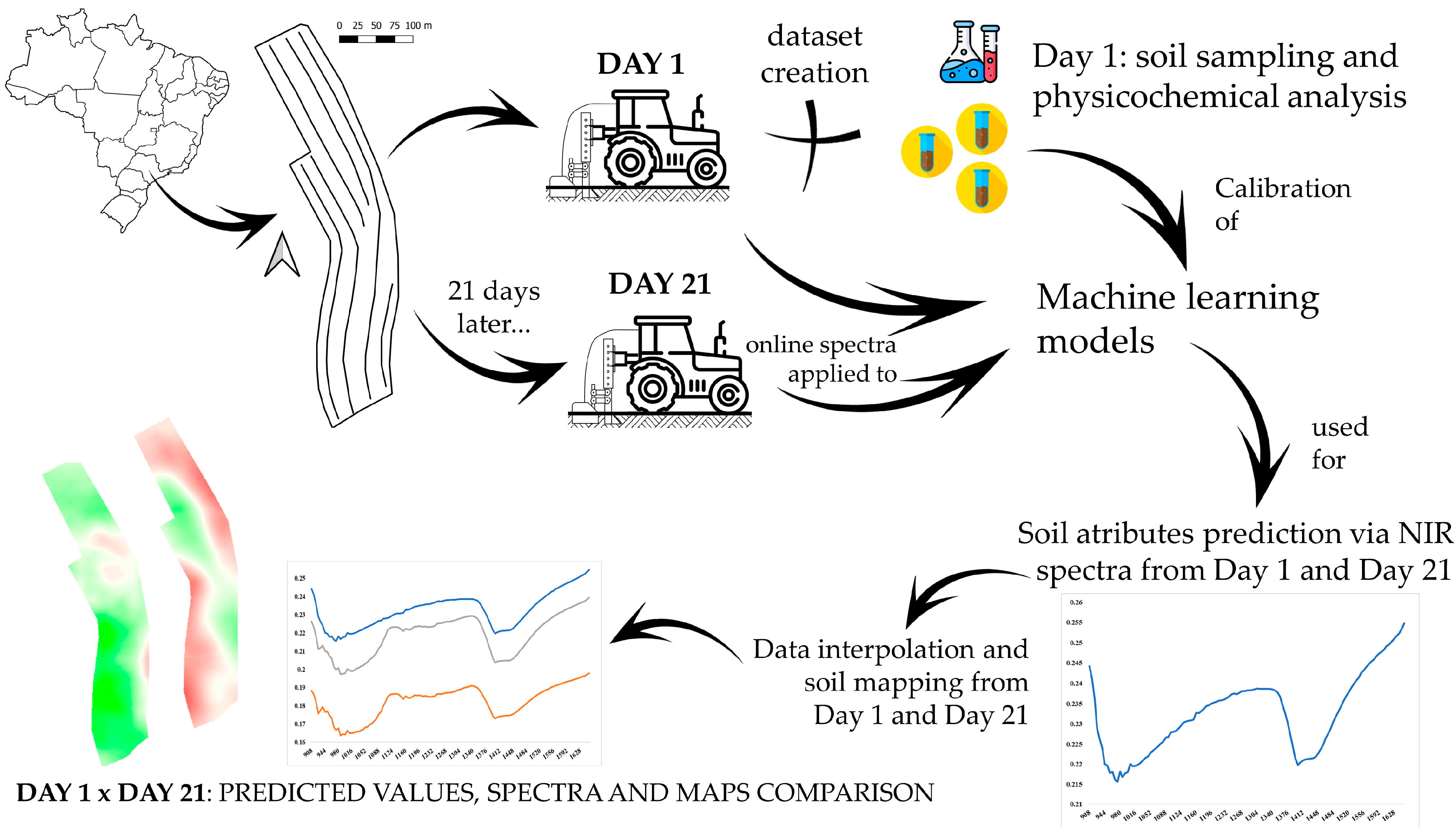
2. Material and Methods
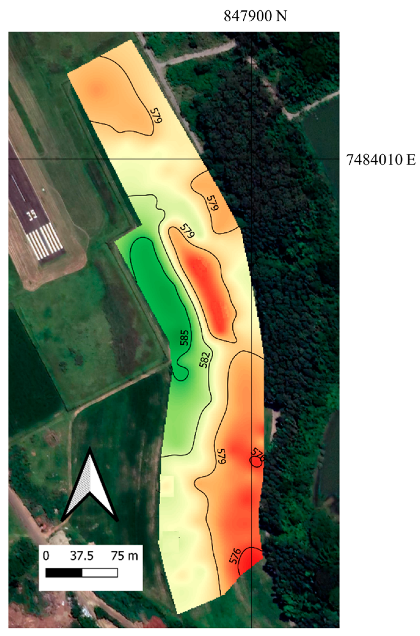
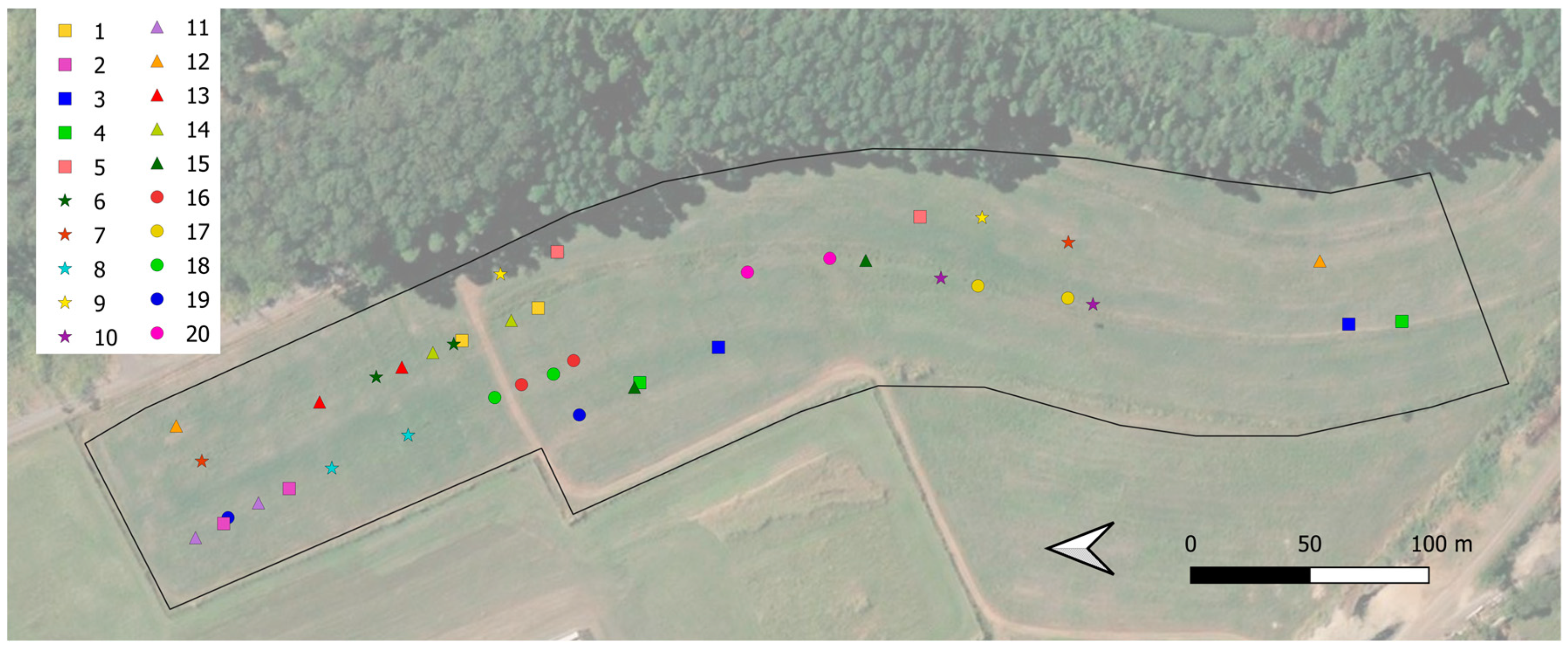
This study was carried out following the steps presented in Figure 1, detailed in Section 2.1, Section 2.2, Section 2.3 and Section 2.4. Only the details regarding the objective of this study are presented. Additional information and specificities can be found in the previous study that aimed to validate the methods and ML models used as the basis for the present study [28].

2.1. Study Area

The study area is a 6.0 ha sandy loam (average of 12% clay) experimental field at the University of São Paulo (USP), located in Piracicaba, state of São Paulo, Brazil (22°43′03.51” S, 47°36′50.03” W). The mean annual temperature and annual total rainfall are 21.6 °C and 1230 mm, respectively (CWa—Köppen classification). In the last three years, a soybean-fallow system was conducted. The study was conducted in November 2021, at the end of the fallow phase, before soybean seeding. During the 21 days that separated the two spectral acquisitions, the area was kept fallow.
The area presents a mid-west highest point of 586 m, with a declivity direction to the south, with the lowest point of 576 m. Two north–south terraces divide the area and delimit the lowest portions at the east. The north portion of the area is a plateau with low altitude variation (Figure 2). The altimetry map was generated due to water topsoil dynamic dependence of altimetry [32,33,34] since soil moisture is known to affect NIR spectra [35,36].

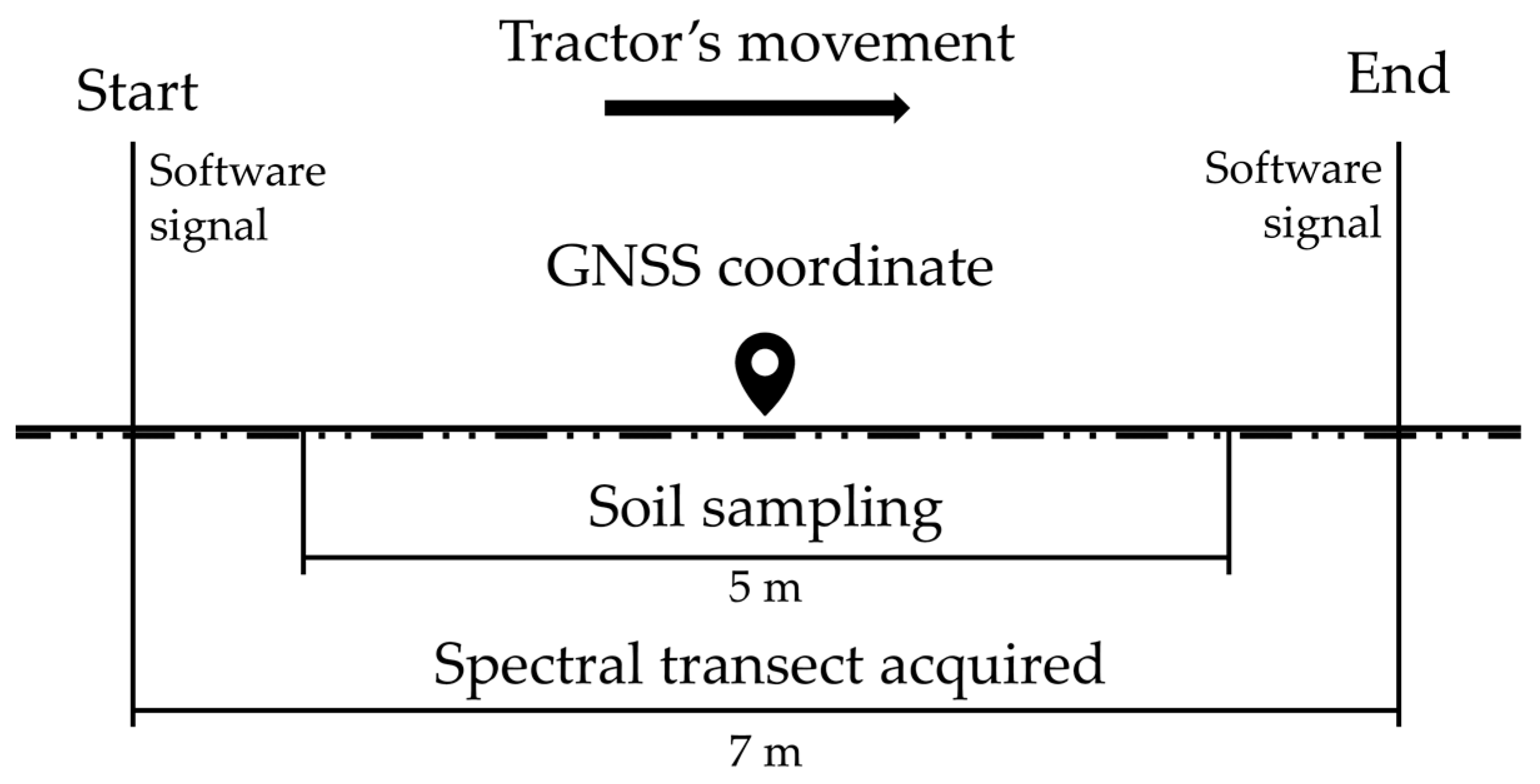
2.2. Online Spectra Acquisition and Soil Sampling

Online soil spectral data were acquired using a subsoiler shank making a 0.15 m-deep furrow, attached to a structure mounted on the three-point hydraulic hitch of a tractor. This shank carried a steel armored case protecting the NIR spectrophotometer (MicroNIR from VIAVI Solutions Inc., Scottsdale, AZ, USA), acquiring 125 wavelength bands from 908.10 to 1676.20 nm with a spectral resolution of 6.14 nm. Acquisition points were georeferenced using a Global Navigation Satellite System (GNSS) Ag-Star (Novatel, Calgary, AB, Canada) receiver with TerraStar-C differential correction (Hexagon, AL, USA).
Two subsequent spectral acquisitions occurred in the area, separated by 21 days. The tractor traveled the area limited by the presence of terraces, making 12 acquisition lines on day 1. The speed was set to 0.583 m s−1 (2.1 km h−1). A total of 383 spectral points were acquired on day 1, followed by a filtering process of measurement errors that excluded 80 spectra. Day 1 was used to validate the methods of spectra acquisition, associated soil sampling, calibrate and evaluate the robustness of ML models for prediction. Data acquisition on day 21 followed the same experimental and instrumental conditions from day 1. Once the models were calibrated and validated, on day 21 only the odd lines of day 1 were acquired, resulting in six acquisition lines and 140 spectra. Then, for the comparison between the spectra and product generated on both days, acquisition from day 1 was reduced to the same lines of day 21 (six acquisition lines), resulting in the same number (140 points) of soil spectra being compared.
Soil sampling occurred on day 1 and was used as reference values to compose the dataset for ML model calibration and evaluation. The soil was sampled in the bottom of the furrow left by the subsoiler shank in the spectral acquisition transect to ensure that soil analysis was correspondent to the area previously sensed. For this, the spectrophotometer acquisition time of one spectrum (10 s) was multiplied by the operation speed, resulting in the transect length sensed (7 m). As the spectrophotometer acquisition software indicates in real-time the starting point of each spectrum, the demarcation of 72 random starting points allowed the afterward soil sampling. To reduce uncertainty, one meter was removed from the beginning and end of each transect sampled, resulting in a five-meter-long soil sample along the furrow (Figure 3). Soil analysis in the laboratory was conducted following the methods described by Teixeira et al. [37]. The attributes and respective analysis methods considered were: clay (HMSF + NaOH); OM (oxidation); CEC, the sum of basis (resin) plus soil total acidity (KCl); pH (CaCl2); P, K, Ca, and Mg (resin).
On each day of acquisition, ten soil samples were randomly collected at the bottom of the furrow left by the subsoiler shank to monitor the soil moisture. These samples were collected during the field operation, sealed, and weighed in field conditions. Then, they were taken to a forced ventilation oven at 105 °C for 72 h to obtain their dry weight [37]. The soil moisture on each day was considered as the mean value for the ten samples collected.

2.3. Machine Learning Models and Data Interpolation

The ML models for soil attributes prediction were calibrated using principal components regression (PCR), a well-described technique applied to cope with multivariate data such as soil NIR spectra, allowing the reduction of noisy, redundant, and sparse data [38,39]. PCR occurs in three steps: (a) a principal components analysis (PCA) is applied in the entire data matrix; (b) a linear regression is used to obtain the vector of estimated regression coefficients; (c) the eigenvectors, as the loadings of PCA are used to obtain the estimators of PCR, as shown in Equation (1).
β k ^ = V k δ k ^
where β ^ = PCR estimator, k belongs to {1, …, p}, p = number of covariants, V = orthonormal set of eigenvectors, δ ^ = coefficients vector of estimated regressors. The number of principal components (PC) used in the regression was set following the criteria of reducing the RMSE and using at most 10 PCs to avoid the model’s overfitting [40,41]. Data modeling was developed using Jupyter Notebook software [42,43]. The dataset composed of online near spectra from day 1’s acquisition and analysis of corresponding soil samples was divided into the proportion of 70% for calibration and 30% for validation. The k-fold cross-validation (k = 10) was applied to reduce the bias of the results reported [44]. The function random state was set to n = 456 to ensure the repeatability of results after validation.
The strategy of using only local samples from the experimental area yielded the best predictions and, therefore, was applied in this study. Further description of ML models applied in this study can be found in the beforementioned paper [28]. These same models were applied to the online spectra acquired on day 21.
After the prediction of the 140 points for both days of acquisition, variograms for each individual attribute were adjusted with the data for posterior interpolation by ordinary kriging, using the software Vesper [45]. Variograms were fitted within the software that provides RMSE and Akaike information criterion (AIC) index for model adjustment. These two parameters are evaluated as minimization parameters since they refer to the error in variogram modeling. Vesper also gives the parameters nugget (C0)—portion of variance that cannot be explained by spatial dependence, sill (C1)—the structural component of the spatial dependence, and range (A)—the minimum distance in meters between samples that present relationship for the evaluated attribute [45]. The method used was block kriging in 3.0 m × 3.0 m pixels, and the minimum and maximum neighboring points for interpolation were set to software minimum and maximum possible values of 4 and 300, respectively. The kriging results were converted to a raster format to be exported and analyzed in a geographic information system software.

2.4. Prediction Values, Spectra Characteristics, and Maps Analysis

Three populations were created to be compared:
  • Overlap population: an ellipse buffer of 2.5 m radius in the direction of the tractor’s movement was created to extract overlap points, as the soil sampling was carried in the length of five meters to match the transect of spectral acquisition (see Section 2.2). This analysis was considered since, at the field operation, two spectra would hardly be acquired at the same point. Although the tractor’s operator, operation speed, and acquisition lines were the same, variations in orientation or border maneuvers could offset the spectra from day 21 from the location of day 1. This would hinder the direct comparison of day 1 vs day 21 as: spectrumday1 1 vs. spectrumday21 1; spectrumday1 n vs. spectrumday21 n; …; spectrumday1 140 vs. spectrumday21 140;
  • High correlated population: the 20 highest correlated spectra pairs (day 1 vs. day 21) were identified using Pearson’s correlation analysis. For this purpose, the 125 wavelengths measured were the variables compared for spectra correlation;
  • Total population: the nearest neighbors from day 1 and day 21 were joined in pairs, yielding 140 pairs used for correlation analysis. The total population was of higher attention in our study since its analysis can lead to understanding if field management decisions based on the predictive performance of the models over time would be stable and, therefore, reliable—the main goal of this study.
A 99% significance (p < 0.01) Pearson’s correlation analysis was used to compare the prediction values between day 1 and day 21 of the three populations (total, highly correlated, and overlap). The correlation among soil attributes on day 1 and day 21 predictions, as well as the statistical distribution of values predicted, were evaluated considering all the 140 spectra from the two days, using r and kernel density estimate function.
Spectra characteristics such as morphology, intensity, and absorption features were also compared. These are important characteristics affected by mineralogy, texture, OM content, and soil moisture [8]. The location of spectra acquisition was compared for the highly correlated population to verify if the high correlation in reflectance values of spectral bands meant they were acquired in near locations.
The maps were generated using the total population due to its higher density of sample points compared to the other two populations. The comparison was aimed to assess the similarity between the final products of DRS NIR soil attributes prediction from day 1 and day 21. For that, C0, C1, and A parameters from the variograms fitted for day 1 and day 21 values were compared. Also, kriged values converted to raster format were exported to QGIS software [46] to spatialize the differences of prediction in the experimental area. Individually, each attribute difference of prediction was obtained by subtracting the map of day 1 from the map of day 21. Positive values in the residual map mean day 21 overestimated the prediction from day 1, and if the opposite, underestimated.

3. Results and Discussion

The results for k-fold cross-validation of ML models used in this study are presented in Table 1, and their validation is reported in the previous study [28]. Primary response attributes, clay and OM, have well-known wavelengths of response [10,47]. Both clay and OM models allowed robust mapping of the experimental area, although clay reported a considered low R2 = 0.17. Of secondary response attributes, CEC model successfully achieved the field patterns of those observed in laboratory analysis, presenting an accurate prediction of R2 = 0.60 and RMSE = 3.51 mmolc kg−1. The poor parameters, especially of R2, of 0.03 for pH, 0.02 for P, 0.14 for K, 0.39 for Ca, and 0.01 for Mg was confirmed as poor prediction results.

3.1. Prediction Values, Spectra Characteristics, and Maps Analysis

Almost all the predicted values of day 1 and day 21 presented a low correlation (Table 2). The significative but negative Pearson correlation coefficient (r) values presented by pH and P are not of agronomic interest for use in the ML models since they denote that zones predicted with high values on day 1 were inverted into zones of low P and pH values on day 21, and vice versa. The pH significative r appeared only for the total population, being −0.26. P prediction had an alternate distribution in the three populations comparison, represented by the r of −0.73, −0.80, and −0.56 for overlap, highly correlated, and total population spectra, respectively.
The attribute P has no direct response in NIR spectra, and its successful prediction is hardly obtained with this technique, particularly in tropical soils, because of the great adsorption specificity of this attribute with iron and aluminum oxides, and 1:1 clay minerals such as kaolinite [48]. Usually, the best predictions of P are observed in temperate soils, especially those under organic fertilization, since the organic amendments compete for site-specific P adsorption, leaving more P labile [49]. In this situation, a positive correlation is frequently observed between P and OM. The last one is a direct NIR response attribute that allows to map P using the technique. In this context (tropical soils), the P prediction was not expected to work properly in the present study.
However, the inversion of patterns in P prediction can further indicate that when the model identifies no pattern for an attribute, it will randomly assign values depending on the conditions of the spectra. Therefore, using DRS NIR spectra for indirect calibrations have to be strictly used after a covariation analysis with primary attributes in the desirable area [8,39]. As a random attribution of values will follow, there is the risk of still presenting a reasonable prediction, but the absence of causality in this situation hinders the leverage of the technique to be used as a reliable PA tool.

3.1.1. Overlap Population

The overlap predictions represent those spectra acquired in the same location in the area. The greatest positive correlation was observed for Ca prediction, with r = 0.33. Nevertheless, attributes like clay, OM, CEC, and Mg were nearly independent between day 1 and day 21 predictions, while pH, P, and K had negative correlations, which are also not desirable for the use of a ML calibration of NIR spectra over time. Especially for primary NIR attributes, these contents are well-known for being stable in an agricultural area over a short-medium period, either for clay that changes along soil weathering stages [50] or for OM, even with long-term applications and conservationist management [51,52]. The predictions for these attributes separated by 21 days, as was made in this study, were expected to reach similar values.

3.1.2. Highly Correlated Population

The highly correlated pairs from day 1 and day 21 had their r ranging from 0.76–0.91, and all were significant at 99% (p < 0.01). The spectra intensity was higher on day 1 on 16 of the 20 most correlated pairs, which can denote an influence of soil moisture on its acquisition on day 21, reducing the reflectance [22,36,47]. On day 1, the soil gravimetric moisture (θ) was 4.16%, while on day 21, θ was 6.95%. Water has an effect on DRS NIR spectra of augmenting absorption [9,22,36,47]. The interaction of energy with matter can happen as transmission, reflection, or absorption [53]. The higher the absorption, the lower the reflectance. Even a tender rise in soil moisture could have reduced the mean reflectance values from approximately 0.135–0.145 to 0.110–0.120.
For the spectra morphology, similar shapes and absorption features can be observed along the wavelengths of NIR spectra. Figure 4 exemplifies two pairs of correlated spectra separated by approximately 30 m. As was observed by other authors, the primary attributes have characteristic wavelengths of interaction [35,47]. Despite the fact that the data acquisition occurred within a range of 21 days, the sensor perceived the same soil-spectra peculiarities, implying that the core of the DRS technique was maintained on both acquisition days.
Analyzing the location of the 20-most correlated day 1 vs. day 21 spectra pairs, a distance between 20 and 40 m was observed in 12 of these pairs (Figure 5). The other pairs were separated by more than 40 m. The pair represented by the orange triangle, for example, were separated by up to 500 m. This implies that the correlation of 8 out of the 20 most correlated pairs (or 40%) was not due to the proximity in the field, as it was expected and observed for the other 60%. Despite two locations with similar contents, in quantity and quality, of primary NIR response attributes would probably yield highly correlated spectra since the sensor would perceive the same wavelengths of response [8,23,35], this was not the case since the predicted values for the high correlated population had no positive and significative correlation, as observed in Table 2 (Section 3.1). Therefore, this indicates that in whichever way the wavebands of a spectra present correlation, similar shape, or absorption features, the ML models also consider other characteristics for the attribute’s quantification. Perchance, the spectra intensity is one of the major characteristics considered, as properties such as moisture, mineralogy, clay content, and OM directly affect the reflectance intensity [8,54].

3.1.3. Total Population

The total population presented the only positive and significant correlation, for Ca prediction, with r = 0.22. As Ca is a secondary NIR response attribute, therefore depending on the prediction of a primary NIR attribute, and neither of these showed a significative correlation, its exceptional 99% significative correlated prediction indicates no causal relation.
The mean spectra from day 1 and day 21 showed that the intensity of reflectance was higher on day 1 (Figure 6), corroborating the spectra intensity observed for the highly correlated population and the possible implication of the higher soil moisture observed in the acquisition of day 21.
As a possible result of this reduced spectra intensity on day 21, the KDE plots showed a tendency of overestimation of clay content in comparison with day 1 (Figure 7). Both water and clay had a positive influence in absorption features of NIR spectra and a negative influence on spectra intensity [36,54], and overtones of water and clay can also be observed in the same wavelengths [8,47]. Soil moisture was 2.79% higher in the acquisition of day 21. As the physical properties of soils dictate that the higher the clay content, the higher the water-holding capacity due to micropores augmentation [55], it can be suggested that the model identified the greater absorption features and lower intensity on day 21 and assigned that to clay content.
The indication of soil moisture as the main or only source of variation is nevertheless doubted, as indicated by the subsequent analysis. The correlation among soil attributes in day 1 and day 21 predictions shows a pattern of intensification in correlations of day 21, despite no relationship being inverted (positive turning to negative, or the contrary), especially observing those of primary NIR attributes (Figure 8). Other attributes that presented a similar pattern to clay—of overestimation on day 21—were CEC, K, and Mg. However, CEC and K prediction was related to the covariation with OM content, as indicated by the independent correlation with clay on day 1, when the ML models were calibrated and validated. OM also has the property of water absorption and regulates negative charges in soil [56,57]. CEC is directly related to the proportion of negative charges per mass unit, and also K and Ca, as their cation forms will be attracted by the negative charges of soil. However, Ca prediction, which also presented a strong correlation with OM, did not present the same pattern of overestimation that would be likely attributed to soil moisture augmentation.
The analysis of maps generated also corroborates other variables than the soil moisture, influencing the lack of correlation between the two days’ prediction. For primary response attributes, OM had a similar A of 23.0 m for day 1 and 21.1 m for day 21. Clay range increased by 50%, 24.1 m on day 1, and 36.8 m on day 21. CEC had the closest values for day 1 and day 21, for C0, C1, and A (Table 3). For pH, P, K, Ca, and Mg, the changes in variogram parameters were expected, not only because of the differences above described in soil spectra of the two days but also due to the inability of ML models to predict these attributes on day 1. As described by Huang et al. [58], outputs generated from gathered data and various processes have sources of errors that can accumulate, especially when applying machine learning to chemistry data [59].
The clay residual map tended to be positive, showing the pattern of day 21 in overestimation compared with the day 1 prediction (Figure 9). However, if moisture was the only factor actuating, traces of water topsoil dynamic would appear in the clay residual map, highlighting the regions where altimetry would conduct the water [32,33,34]. The lower portions of the area, following the altimetry and agricultural terraces, were not where the higher differences in prediction appeared. OM had a more random residual distribution than the observed for clay, with more portions where day 21 underestimated the prediction of day 1, despite the greater soil moisture and related wavelengths of OM and water in NIR spectra [36,47].
The literature recognizes that soil moisture can influence soil attribute prediction using NIR spectra. Alternatives to deal with this factor’s variation in NIR laboratory spectra [9,25,60] should also be considered for online NIR spectra calibrations. Nevertheless, these strategies often use the consecutive spectral acquisition of soil samples in different moisture contents. Authors resort to soil drying and rewetting and then build ML calibrations that consider the moisture level in prediction. This may be a challenge to applying for online spectra since the acquisition must be made in field conditions.
Despite that, the scenario presented in this study leads to conclude that:
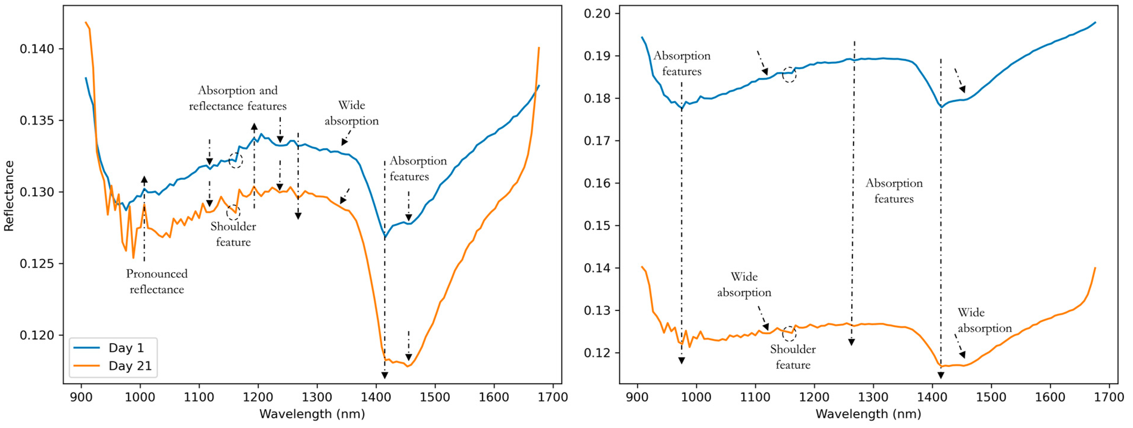
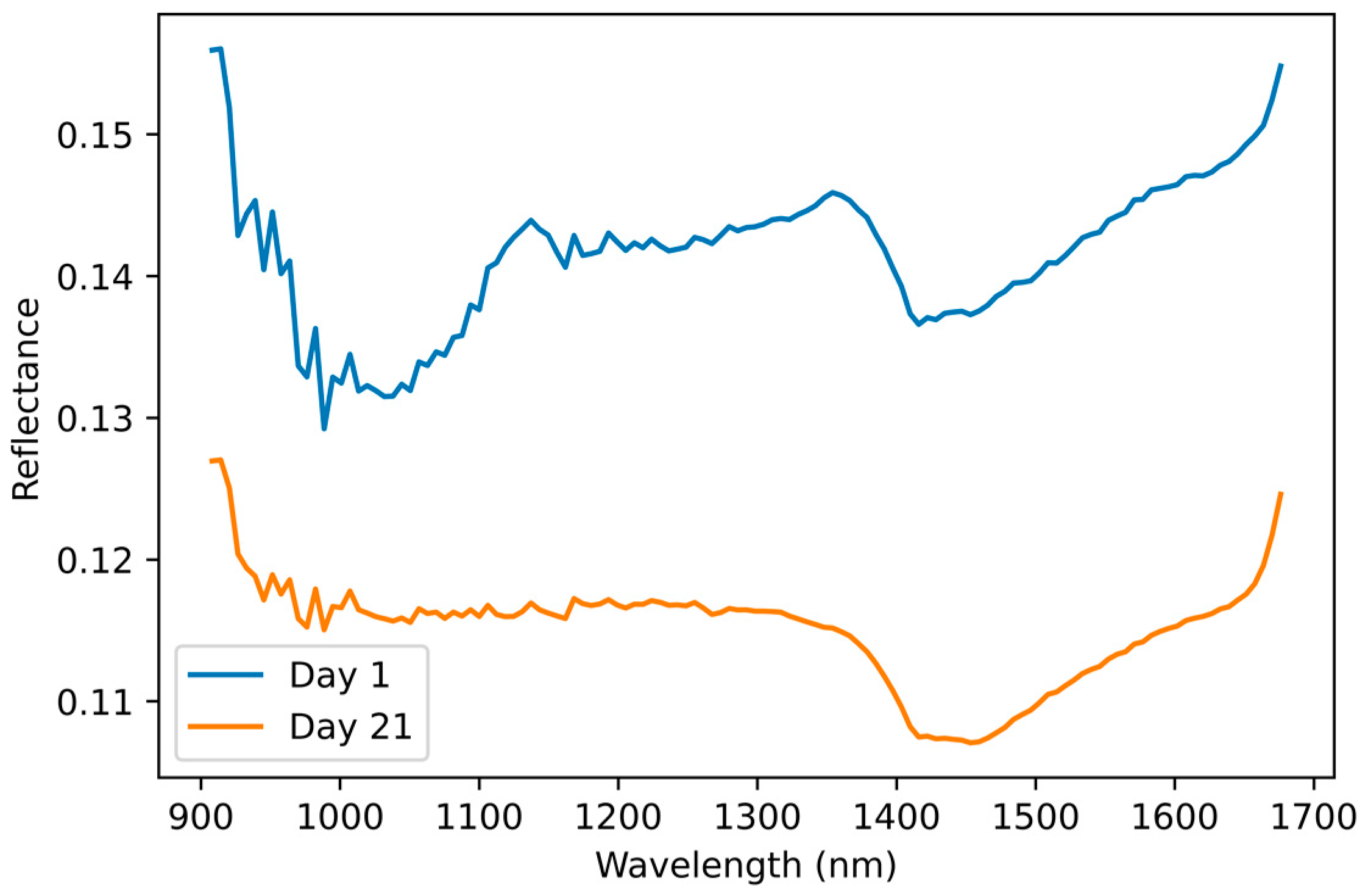
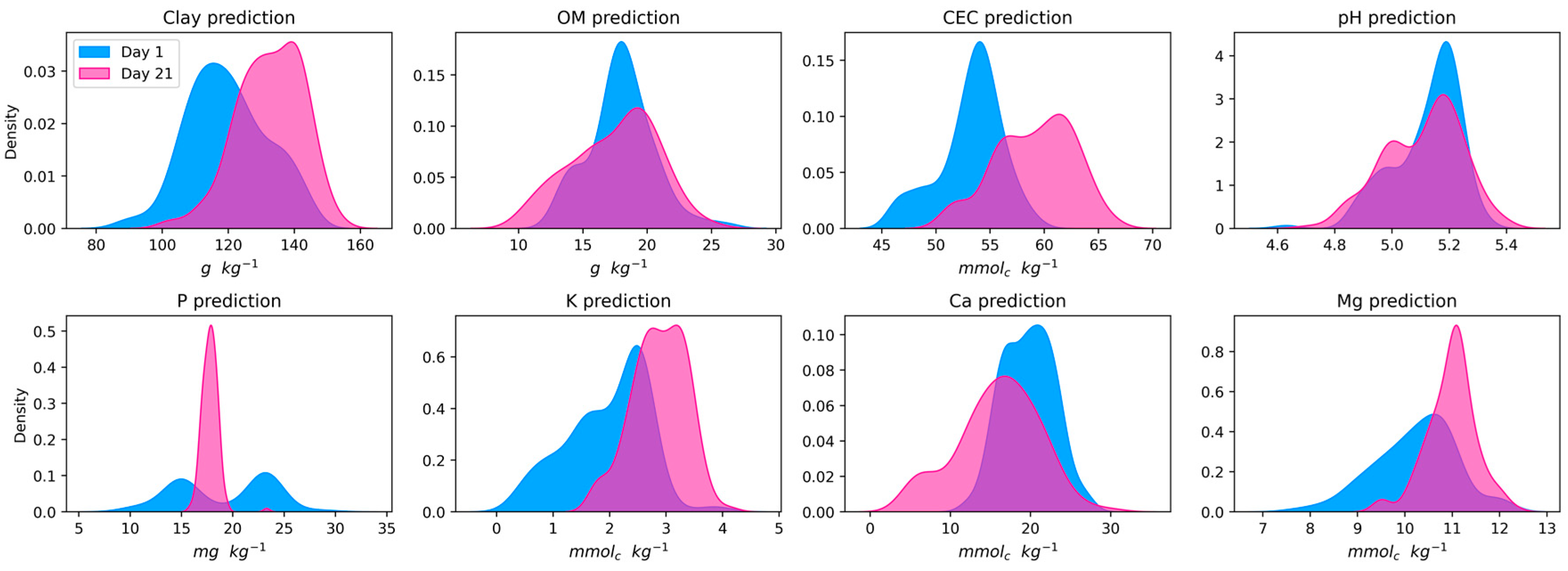
  • Water could intensify the values predicted. However, this may not be the only explanation for the differences in day 21 spectra prediction using ML models calibrated on day 1. The analysis of predicted values, as shown in Table 2, are not intensified but almost independent from each other;
  • Other environmental factors must be interfering in spectra acquisition, which can explain the differences between the two days’ predictions. Since it is harder to control the circumstances of a field operation than of a laboratory, any peculiarity can change the aspects of acquired spectra. One possibility to be tested is the measuring chamber designed and validated by Rodionov et al. [61]. No other studies report a methodology to isolate the visible-NIR spectra acquisition during field operations, simulating a laboratory condition, as the usual is the subsoiler shank and spectrophotometer being carried in an open field. This strategy can be tested for acquisitions over time since spectral acquisition will still suffer from topsoil particle size variation, soil moisture, and tractor movement but can isolate other environmental factors.
  • A further investigation into factors such as sunlight, soil temperature, air temperature, etc., needs to be carried out. This means investigating the possibility of providing the models’ auxiliary data to deal with spectra variation and guaranteeing more stability for the ML calibrations which depend on it.
This study may lead to different analyses of online NIR spectra. Other factors not mentioned in this study can also be proposed as sources of variation. The elucidation of these questions may clarify to the DRS community if there are strategies to consolidate the stability of online NIR spectra over time. In the current scenario, the prediction of soil attributes using DRS in the NIR region indicates the need for spatio-temporal local calibrations, and further strategies to turn the technique more sustainable and economically feasible are necessary to leverage it into agricultural production.

4. Conclusions

Validated ML models of online NIR spectra for soil attributes prediction were submitted to a test of performance over time. The analysis considered spectra in overlapped locations between the two days, highly correlated spectra pairs, and the total population of day 1 x day 21. The initial hypothesis of online spectra spatio-temporal stability is not supported. Overlapped spectra presented independent values in prediction. Highly correlated spectra between the two days were observed independently of the distance of acquisition in the field. However, high spectra correlation did not mean a correlation of values predicted. The total populations had their only significative correlation for an indirect NIR attribute, but no causal relation was found. The values predicted, statistical distribution, and spatial distribution of residuals between day 1 and day 21 suggested that soil moisture was not the only source of variation. Therefore, ML models calibrated on the first day did not perform as consistently when used spectra acquired on day 21, suggesting the requirement of spatio-temporal local calibrations for DRS NIR prediction of soil attributes.

Author Contributions

Conceptualization, R.C.F. and J.P.M.; methodology, R.C.F. and J.P.M.; formal analysis, R.C.F. and J.P.M.; investigation, R.C.F.; writing—original draft preparation, R.C.F.; writing—review and editing, R.C.F., M.C.F.W., E.R.O.d.S. and J.P.M.; validation, R.C.F., M.C.F.W., E.R.O.d.S. and J.P.M.; visualization, R.C.F., M.C.F.W., E.R.O.d.S. and J.P.M.; supervision, J.P.M.; funding acquisition, J.P.M. All authors have read and agreed to the published version of the manuscript.

Funding

Soil sample analyses were funded by the Brazilian Institute of Analysis (IBRA). The sensor was offered from a partnership with Spectral Solutions (São Paulo, Brazil). R.C.F. was funded by the National Council for Scientific and Technological Development (CNPq)—Project 830707/1999-9.

Data Availability Statement

Not applicable.

Conflicts of Interest

The authors declare no conflict of interest.

References

  1. International Society of Precision Agriculture. Precision Agriculture Definition; International Society of Precision Agriculture: Monticello, IL, USA, 2021. [Google Scholar]
  2. Molin, J.P.; Tavares, T.R. Sensor Systems for Mapping Soil Fertility Attributes: Challenges, Advances, and Perspectives in Brazilian Tropical Soils. Eng. Agric. 2019, 39, 126–147. [Google Scholar] [CrossRef] [Green Version]
  3. Yin, H.; Cao, Y.; Marelli, B.; Zeng, X.; Mason, A.J.; Cao, C. Soil Sensors and Plant Wearables for Smart and Precision Agriculture. Adv. Mater. 2021, 33, 2007764. [Google Scholar] [CrossRef] [PubMed]
  4. Johnston, A.E.; Poulton, P.R. The Importance of Long-Term Experiments in Agriculture: Their Management to Ensure Continued Crop Production and Soil Fertility; the Rothamsted Experience. Eur. J. Soil Sci. 2018, 69, 113–125. [Google Scholar] [CrossRef] [PubMed] [Green Version]
  5. Foley, J.A.; DeFries, R.; Asner, G.P.; Barford, C.; Bonan, G.; Carpenter, S.R.; Chapin, F.S.; Coe, M.T.; Daily, G.C.; Gibbs, H.K.; et al. Global Consequences of Land Use. Science 2005, 309, 570–574. [Google Scholar] [CrossRef] [PubMed] [Green Version]
  6. Smith, P.; House, J.I.; Bustamante, M.; Sobocká, J.; Harper, R.; Pan, G.; West, P.C.; Clark, J.M.; Adhya, T.; Rumpel, C.; et al. Global Change Pressures on Soils from Land Use and Management. Glob. Chang. Biol. 2016, 22, 1008–1028. [Google Scholar] [CrossRef]
  7. Vasques, G.M.; Rodrigues, H.M.; Coelho, M.R.; Baca, J.F.M.; Dart, R.O.; Oliveira, R.P.; Teixeira, W.G.; Ceddia, M.B. Field Proximal Soil Sensor Fusion for Improving High-Resolution Soil Property Maps. Soil Syst. 2020, 4, 52. [Google Scholar] [CrossRef]
  8. Stenberg, B.; Viscarra Rossel, R.A.; Mouazen, A.M.; Wetterlind, J. Visible and Near Infrared Spectroscopy in Soil Science. In Advances in Agronomy; Elsevier: Amsterdam, The Netherlands, 2010; Volume 107. [Google Scholar]
  9. Nocita, M.; Stevens, A.; Noon, C.; Van Wesemael, B. Prediction of Soil Organic Carbon for Different Levels of Soil Moisture Using Vis-NIR Spectroscopy. Geoderma 2013, 199, 37–42. [Google Scholar] [CrossRef]
  10. Fang, Q.; Hong, H.; Zhao, L.; Kukolich, S.; Yin, K.; Wang, C. Visible and Near-Infrared Reflectance Spectroscopy for Investigating Soil Mineralogy: A Review. J. Spectrosc. 2018, 2018, 3168974. [Google Scholar] [CrossRef]
  11. Bönecke, E.; Meyer, S.; Vogel, S.; Schröter, I.; Gebbers, R.; Kling, C.; Kramer, E.; Lück, K.; Nagel, A.; Philipp, G.; et al. Guidelines for Precise Lime Management Based on High-Resolution Soil PH, Texture and SOM Maps Generated from Proximal Soil Sensing Data. Precis. Agric. 2021, 22, 493–523. [Google Scholar] [CrossRef]
  12. Munnaf, M.A.; Guerrero, A.; Nawar, S.; Haesaert, G.; Van Meirvenne, M.; Mouazen, A.M. A Combined Data Mining Approach for On-Line Prediction of Key Soil Quality Indicators by Vis-NIR Spectroscopy. Soil Tillage Res. 2021, 205, 104808. [Google Scholar] [CrossRef]
  13. Wang, Y.; Huang, T.; Liu, J.; Lin, Z.; Li, S.; Wang, R.; Ge, Y. Soil PH Value, Organic Matter and Macronutrients Contents Prediction Using Optical Diffuse Reflectance Spectroscopy. Comput. Electron. Agric. 2015, 111, 69–77. [Google Scholar] [CrossRef]
  14. Munnaf, M.A.; Nawar, S.; Mouazen, A.M. Estimation of Secondary Soil Properties by Fusion of Laboratory and On-Line Measured Vis-NIR Spectra. Remote Sens. 2019, 11, 2819. [Google Scholar] [CrossRef] [Green Version]
  15. Munnaf, M.A.; Mouazen, A.M. Development of a Soil Fertility Index Using On-Line Vis-NIR Spectroscopy. Comput. Electron. Agric. 2021, 188, 106341. [Google Scholar] [CrossRef]
  16. Yang, M.; Mouazen, A.; Zhao, X.; Guo, X. Assessment of a Soil Fertility Index Using Visible and Near-Infrared Spectroscopy in the Rice Paddy Region of Southern China. Eur. J. Soil Sci. 2020, 71, 615–626. [Google Scholar] [CrossRef]
  17. Viscarra Rossel, R.A.; Adamchuk, V.I.; Sudduth, K.A.; McKenzie, N.J.; Lobsey, C. Proximal Soil Sensing. An Effective Approach for Soil Measurements in Space and Time. Adv. Agron. 2011, 113, 243–291. [Google Scholar] [CrossRef]
  18. Ben-Dor, E.; Heller, D.; Chudnovsky, A. A Novel Method of Classifying Soil Profiles in the Field Using Optical Means. Soil Sci. Soc. Am. J. 2008, 72, 1113–1123. [Google Scholar] [CrossRef]
  19. Mouazen, A.M.; Maleki, M.R.; Cockx, L.; Van Meirvenne, M.; Van Holm, L.H.J.; Merckx, R.; De Baerdemaeker, J.; Ramon, H. Optimum Three-Point Linkage Set up for Improving the Quality of Soil Spectra and the Accuracy of Soil Phosphorus Measured Using an on-Line Visible and near Infrared Sensor. Soil Tillage Res. 2009, 103, 144–152. [Google Scholar] [CrossRef] [Green Version]
  20. Stenberg, B.; Rogstrand, G.; Bölenius, E.; Arvidsson, J. On-Line Soil NIR Spectroscopy: Identification and Treatment of Spectra Influenced by Variable Probe Distance and Residue Contamination. In Proceedings of the 6th European Conference on Precision Agriculture: ECPA 2007, Skiathos, Greece, 3–6 June 2007. [Google Scholar]
  21. Barra, I.; Haefele, S.M.; Sakrabani, R.; Kebede, F. Soil Spectroscopy with the Use of Chemometrics, Machine Learning and Pre-Processing Techniques in Soil Diagnosis: Recent Advances—A Review. TrAC—Trends Anal. Chem. 2021, 135, 116166. [Google Scholar] [CrossRef]
  22. Morellos, A.; Pantazi, X.E.; Moshou, D.; Alexandridis, T.; Whetton, R.; Tziotzios, G.; Wiebensohn, J.; Bill, R.; Mouazen, A.M. Machine Learning Based Prediction of Soil Total Nitrogen, Organic Carbon and Moisture Content by Using VIS-NIR Spectroscopy. Biosyst. Eng. 2016, 152, 104–116. [Google Scholar] [CrossRef] [Green Version]
  23. Kuang, B.; Mahmood, H.S.; Quraishi, M.Z.; Hoogmoed, W.B.; Mouazen, A.M.; van Henten, E.J. Sensing Soil Properties in the Laboratory, in Situ, and on-Line. A Review. In Advances in Agronomy; Elsevier: Amsterdam, The Netherlands, 2012; Volume 114. [Google Scholar]
  24. Eitelwein, M.T.; Tavares, T.R.; Molin, J.P.; Trevisan, R.G.; de Sousa, R.V.; Demattê, J.A.M. Predictive Performance of Mobile Vis—NIR Spectroscopy for Mapping Key Fertility Attributes in Tropical Soils through Local Models Using PLS and ANN. Automation 2022, 3, 116–131. [Google Scholar] [CrossRef]
  25. Franceschini, M.H.D.; Demattê, J.A.M.; Kooistra, L.; Bartholomeus, H.; Rizzo, R.; Fongaro, C.T.; Molin, J.P. Effects of External Factors on Soil Reflectance Measured On-the-Go and Assessment of Potential Spectral Correction through Orthogonalisation and Standardisation Procedures. Soil Tillage Res. 2018, 177, 19–36. [Google Scholar] [CrossRef]
  26. Nawar, S.; Mouazen, A.M. Optimal Sample Selection for Measurement of Soil Organic Carbon Using On-Line Vis-NIR Spectroscopy. Comput. Electron. Agric. 2018, 151, 469–477. [Google Scholar] [CrossRef]
  27. Brown, D.J. Using a Global VNIR Soil-Spectral Library for Local Soil Characterization and Landscape Modeling in a 2nd-Order Uganda Watershed. Geoderma 2007, 140, 444–453. [Google Scholar] [CrossRef]
  28. Canal Filho, R.; Molin, J.P. Spatial Distribution as a Key Factor for Evaluation of Soil Attributes Prediction at Field Level Using Online Near-Infrared Spectroscopy. Front. Soil Sci. 2022, 2, 984963. [Google Scholar] [CrossRef]
  29. Wetterlind, J.; Stenberg, B.; Söderström, M. Increased Sample Point Density in Farm Soil Mapping by Local Calibration of Visible and near Infrared Prediction Models. Geoderma 2010, 156, 152–160. [Google Scholar] [CrossRef] [Green Version]
  30. Gogé, F.; Gomez, C.; Jolivet, C.; Joffre, R. Which Strategy Is Best to Predict Soil Properties of a Local Site from a National Vis-NIR Database? Geoderma 2014, 213, 1–9. [Google Scholar] [CrossRef]
  31. Stevens, A.; Nocita, M.; Tóth, G.; Montanarella, L.; van Wesemael, B. Prediction of Soil Organic Carbon at the European Scale by Visible and Near InfraRed Reflectance Spectroscopy. PLoS ONE 2013, 8, e66409. [Google Scholar] [CrossRef]
  32. Lee, H.; Beighley, R.E.; Alsdorf, D.; Jung, H.C.; Shum, C.K.; Duan, J.; Guo, J.; Yamazaki, D.; Andreadis, K. Characterization of Terrestrial Water Dynamics in the Congo Basin Using GRACE and Satellite Radar Altimetry. Remote Sens Env. 2011, 115, 3530–3538. [Google Scholar] [CrossRef] [Green Version]
  33. Uebbing, B.; Forootan, E.; Braakmann-Folgmann, A.; Kusche, J. Inverting Surface Soil Moisture Information from Satellite Altimetry over Arid and Semi-Arid Regions. Remote Sens. Environ. 2017, 196, 205–223. [Google Scholar] [CrossRef] [Green Version]
  34. Orth, R.; Koster, R.D.; Seneviratne, S.I. Inferring Soil Moisture Memory from Streamflow Observations Using a Simple Water Balance Model. J. Hydrometeorol. 2013, 14, 1773–1790. [Google Scholar] [CrossRef]
  35. Pasquini, C. Near Infrared Spectroscopy: A Mature Analytical Technique with New Perspectives—A Review. Anal. Chim. Acta 2018, 1026, 8–36. [Google Scholar] [CrossRef] [PubMed]
  36. Wang, Y.P.; Lee, C.K.; Dai, Y.H.; Shen, Y. Effect of Wetting on the Determination of Soil Organic Matter Content Using Visible and Near-Infrared Spectrometer. Geoderma 2020, 376, 114528. [Google Scholar] [CrossRef]
  37. Teixeira, P.C.; Donagemma, G.K.; Fontana, A.; Teixeira, W.G. Manual de Métodos de Análise de Solo; Embrapa: Brasilia, Brazil, 2017; Volume 3. [Google Scholar]
  38. Agarwal, A.; Shah, D.; Shen, D.; Song, D. On Robustness of Principal Component Regression. In Advances in Neural Information Processing Systems; NeurIPS: New Orleans, LA, USA, 2021; Volume 116. [Google Scholar] [CrossRef]
  39. Chang, C.W.; Laird, D.A.; Mausbach, M.J.; Hurburgh, C.R. Near-infrared reflectance spectroscopy–principal components regression analyses of soil properties. Soil Sci. Soc. Am. J. 2001, 65, 480–490. [Google Scholar] [CrossRef] [Green Version]
  40. Seasholtz, M.B.; Kowalski, B. The Parsimony Principle Applied to Multivariate Calibration. Anal Chim. Acta 1993, 277, 165–177. [Google Scholar] [CrossRef]
  41. Tracy, T.; Fu, Y.; Roy, I.; Jonas, E.; Glendenning, P. Towards Machine Learning on the Automata Processor. In High Performance Computing, Proceedings of the 31st International Conference, ISC High Performance 2016, Frankfurt, Germany, 19–23 June 2016; Springer: Berlin/Heidelberg, Germany, 2016; Volume 9697, p. 9697. [Google Scholar]
  42. Kluyver, T.; Ragan-Kelley, B.; Pérez, F.; Granger, B.; Bussonnier, M.; Frederic, J.; Kelley, K.; Hamrick, J.; Grout, J.; Corlay, S.; et al. Jupyter Notebooks—A Publishing Format for Reproducible Computational Workflows. In Positioning and Power in Academic Publishing: Players, Agents and Agendas, Proceedings of the 20th International Conference on Electronic Publishing, Göttingen, Germany, 7–9 June 2016; ELPUB: Stuttgart, Germany, 2016. [Google Scholar]
  43. Python Software 3.9.12; Foundation Python: Wilmington, DE, USA, 2022.
  44. Jung, Y. Multiple Predicting K-Fold Cross-Validation for Model Selection. J. Nonparametr. Stat. 2018, 30, 197–215. [Google Scholar] [CrossRef]
  45. Minasny, B.; McBratney, A.B.; Whelan, B.M. VESPER, Version 1.62; Australian Centre for Precision Agriculture, The University of Sydney: Sydney, Australia, 2006. [Google Scholar]
  46. QGIS Development Team. QGIS Geographic Information System; QGIS: London, UK, 2022. [Google Scholar]
  47. Nocita, M.; Stevens, A.; van Wesemael, B.; Aitkenhead, M.; Bachmann, M.; Barthès, B.; Ben-Dor, E.; Brown, D.J.; Clairotte, M.; Csorba, A.; et al. Soil Spectroscopy: An Alternative to Wet Chemistry for Soil Monitoring. Adv. Agron. 2015, 132, 139–159. [Google Scholar] [CrossRef]
  48. Pavinato, P.S.; Cherubin, M.R.; Soltangheisi, A.; Rocha, G.C.; Chadwick, D.R.; Jones, D.L. Revealing Soil Legacy Phosphorus to Promote Sustainable Agriculture in Brazil. Sci. Rep. 2020, 10, 15615. [Google Scholar] [CrossRef] [PubMed]
  49. Mouazen, A.M.; Kuang, B. On-Line Visible and near Infrared Spectroscopy for in-Field Phosphorous Management. Soil Tillage Res. 2016, 155, 471–477. [Google Scholar] [CrossRef]
  50. Jackson, M.L.; Sherman, G.D. Chemical Weathering of Minerals in Soils. Adv. Agron. 1953, 5, 219–318. [Google Scholar] [CrossRef]
  51. Lu, Y.; Gao, Y.; Nie, J.; Liao, Y.; Zhu, Q. Substituting Chemical P Fertilizer with Organic Manure: Effects on Double-Rice Yield, Phosphorus Use Efficiency and Balance in Subtropical China. Sci. Rep. 2021, 11, 8629. [Google Scholar] [CrossRef]
  52. Wang, H.; Xu, J.; Liu, X.; Zhang, D.; Li, L.; Li, W.; Sheng, L. Effects of Long-Term Application of Organic Fertilizer on Improving Organic Matter Content and Retarding Acidity in Red Soil from China. Soil Tillage Res. 2019, 195, 104382. [Google Scholar] [CrossRef]
  53. Kortüm, G.; Braun, W.; Herzog, G. Principles and Techniques of Diffuse-Reflectance Spectroscopy. Angew. Chem. Int. Ed. Engl. 1963, 2, 333–341. [Google Scholar] [CrossRef]
  54. Terra, F.S.; Demattê, J.A.M.; Viscarra Rossel, R.A. Proximal Spectral Sensing in Pedological Assessments: Vis-NIR Spectra for Soil Classification Based on Weathering and Pedogenesis. Geoderma 2018, 318, 123–136. [Google Scholar] [CrossRef]
  55. Rasa, K.; Heikkinen, J.; Hannula, M.; Arstila, K.; Kulju, S.; Hyväluoma, J. How and Why Does Willow Biochar Increase a Clay Soil Water Retention Capacity? Biomass Bioenergy 2018, 119, 346–353. [Google Scholar] [CrossRef]
  56. Shepherd, M.A.; Harrison, R.; Webb, J. Managing Soil Organic Matter—Implications for Soil Structure on Organic Farms. Soil Use Manag. 2002, 18, 284–292. [Google Scholar] [CrossRef]
  57. Soane, B.D. The Role of Organic Matter in Soil Compactibility: A Review of Some Practical Aspects. Soil Tillage Res. 1990, 16, 179–201. [Google Scholar] [CrossRef]
  58. Huang, J.; Zare, E.; Malik, R.S.; Triantafilis, J. An Error Budget for Soil Salinity Mapping Using Different Ancillary Data. Soil Res. 2015, 53, 561–575. [Google Scholar] [CrossRef]
  59. Vishwakarma, G.; Sonpal, A.; Hachmann, J. Metrics for Benchmarking and Uncertainty Quantification: Quality, Applicability, and Best Practices for Machine Learning in Chemistry. Trends Chem. 2021, 3, 146–156. [Google Scholar] [CrossRef]
  60. Wijewardane, N.K.; Ge, Y.; Morgan, C.L.S. Moisture Insensitive Prediction of Soil Properties from VNIR Reflectance Spectra Based on External Parameter Orthogonalization. Geoderma 2016, 267, 92–101. [Google Scholar] [CrossRef] [Green Version]
  61. Rodionov, A.; Welp, G.; Damerow, L.; Berg, T.; Amelung, W.; Pätzold, S. Towards on-the-go field assessment of soil organic carbon using Vis-NIR diffuse reflectance spectroscopy: Developing and testing a novel tractor-driven measuring chamber. Soil Tillage Res. 2015, 145, 93–102. [Google Scholar] [CrossRef]
Figure 1. Flowchart of the methodology developed in this study, exemplifying the steps regarding the field data acquisition separated by 21 days, machine learning modeling and subsequent comparisons between day 1 and day 21 spectra.
Agriengineering 05 00074 g001
Figure 2. Altimetry map of the experimental field, with respective contour lines. The higher portions are colored in green tones and the lower portions in red tones.
Agriengineering 05 00074 g002
Figure 3. Spectral acquisition and associated soil sample scheme used in day 1 for prediction models calibration.
Agriengineering 05 00074 g003
Figure 4. Spectra morphology analysis of two pairs of high-correlated spectra presenting comparable shape and absorption features. Arrows and circles highlight common absorption features observed in both spectra compared.
Agriengineering 05 00074 g004
Figure 5. Distribution of the 20 highest correlated spectra pairs (day 1 vs. day 21) in the experimental field. Equal geometric shapes with the same color represent the acquisition location of the corresponding pairs (one spectrum from day 1 and its corresponding spectrum from day 21).
Agriengineering 05 00074 g005
Figure 6. Mean spectra from day 1 and day 21 representing the intensity of reflectance on each acquisition day obtained by averaging the reflectance values of the wavelengths read by the sensor.
Agriengineering 05 00074 g006
Figure 7. Kernel density estimation plots of clay, organic matter (OM), cation exchange capacity (CEC), potential of hydrogen (pH), phosphorus (P), potassium (K), calcium (Ca), and magnesium (Mg) predicted using the 140 online spectra from each acquisition day.
Agriengineering 05 00074 g007
Figure 8. Pearson’s correlation among clay, organic matter (OM), cation exchange capacity (CEC), potential of hydrogen (pH), phosphorus (P), potassium (K), calcium (Ca), and magnesium (Mg) predicted using online NIR spectra from day 1 and day 21 acquisitions.
Agriengineering 05 00074 g008
Figure 9. Maps of clay, organic matter (OM), cation exchange capacity (CEC), potential of hydrogen (pH), phosphorus (P), potassium (K), calcium (Ca), and magnesium (Mg) demonstrating the spatialization of the differences observed in the predictions of the two days, calculated by subtracting Day 21—Day 1.
Agriengineering 05 00074 g009
Table 1. Results of principal components regression models k-fold cross-validation for clay, organic matter (OM), cation exchange capacity (CEC), potential of hydrogen (pH), phosphorus (P), potassium (K), calcium (Ca), and magnesium (Mg).
UnitMin MaxRangeR2RMSEMAENC% Var
Clayg kg−151-1831320.1719.8815.08424.01
OM12-35230.753.112.28940.69
CECmmolc kg−145-68240.603.512.78626.70
pH-4.1-6.82.70.030.320.27412.09
Pmg kg−15-68630.029.398.59318.42
Kmmolc kg−10.4-5.04.60.140.930.77632.68
Ca10-34240.392.542.081058.62
Mg5-22170.011.831.4115.85
min: minimum value inserted in calibration; max: maximum value inserted in calibration; range: range of values inserted in calibration; R2: coefficient of determination; RMSE: root mean squared error; MAE: mean absolute error; NC: number of principal components used in regression; % var: percentage of the total of outcome variance explained.
Table 2. Pearson’s correlation coefficient of predicted values for the three populations considered.
ClayOMCECpHPKCaMg
Overlap−0.100.09−0.11−0.19−0.73 **−0.220.330.13
High correlated−0.060.190.320.04−0.80 **−0.030.240.19
Total−0.02−0.03−0.14−0.26 **−0.56 **−0.010.22 **0.20
OM: organic matter; CEC: cation exchange capacity; pH: potential of hydrogen; P: phosphorus; K: potassium; Ca: calcium; Mg: magnesium. ** 99% significative correlation.
Table 3. Parameters of fitted variograms for predicted attributes using Day1 and Day2 spectral acquisitions for clay, organic matter (OM), cation exchange capacity (CEC), pH and soil available nutrients, phosphorus (P), potassium (K), calcium (Ca), and magnesium (Mg).
Day 1Day 21
ModelC0C1AModelC0C1A
ClaySph13.59102.6024.10Exp42.7159.7036.80
OMExp1.823.8523.00Gau0.0010.1821.10
CECExp0.008.5018.50Gau0.0010.8220.50
pHLin0.000.0188.90Exp0.000.0216.70
PGau0.2421.4032.90Exp0.030.8037.60
KGau0.100.4627.30Lin0.010.1935.90
CaSph5.624.5095.60Gau0.0026.7925.20
MgExp0.420.3246.40Exp0.020.2617.50
C0: nugget; C1: sill; A: range; ratio; Sph: spherical; Exp: exponential; Gau: Gaussian; Lin: linear with sill.
Disclaimer/Publisher’s Note: The statements, opinions and data contained in all publications are solely those of the individual author(s) and contributor(s) and not of MDPI and/or the editor(s). MDPI and/or the editor(s) disclaim responsibility for any injury to people or property resulting from any ideas, methods, instructions or products referred to in the content.

