Article

Analysis of Total Soil Nutrient Content with X-ray Fluorescence Spectroscopy (XRF): Assessing Different Predictive Modeling Strategies and Auxiliary Variables

by
Tiago Rodrigues Tavares
1,*,
Eduardo de Almeida
1,
Carlos Roberto Pinheiro Junior
2,
Angela Guerrero
3,
Peterson Ricardo Fiorio
4 and
Hudson Wallace Pereira de Carvalho
1,*
1
Laboratory of Nuclear Instrumentation (LIN), Center for Nuclear Energy in Agriculture (CENA), University of São Paulo (USP), Piracicaba, São Paulo 13416000, Brazil
2
Department of Soil Science, "Luiz de Queiroz” College of Agriculture (ESALQ), University of São Paulo (USP), Piracicaba, São Paulo 13418900, Brazil
3
Precision Soil and Crop Engineering Group (Precision SCoRing), Department of Environment, Faculty of Bioscience Engineering, Ghent University, Coupure Links 653, Blok B, 1st Floor, 9000 Ghent, Belgium
4
Department of Biosystems Engineering, “Luiz de Queiroz” College of Agriculture (ESALQ), University of São Paulo (USP), Piracicaba, São Paulo 13418900, Brazil
*
Authors to whom correspondence should be addressed.
AgriEngineering 2023, 5(2), 680-697; https://doi.org/10.3390/agriengineering5020043
Submission received: 28 February 2023 / Revised: 21 March 2023 / Accepted: 29 March 2023 / Published: 1 April 2023

Abstract

:
The difference in the matrix present in soil samples from different areas limits the performance of nutrient analysis via XRF sensors, and only a few strategies to mitigate this effect to ensure an accurate analysis have been proposed so far. In this context, this research aimed to compare the performance of different predictive models, including a simple linear regression (RS), multiple linear regression (MLR), partial least-squares regression (PLS), and random forest (RF) models for the prediction of Ca and K in agricultural soils. RS models were evaluated on XRF data without (RS1) and with (RS2) Compton normalization. In addition, it was assessed whether using soil texture information and/or vis–NIR spectra as auxiliary variables would optimize the predictive performance of the models. The results showed that all strategies allowed the mitigation of the matrix effect to some degree, enabling the determination of their Ca and K contents with excellent predictive performance (R2 ≥ 0.84). The best performance was obtained using RS2 for the Ca prediction (R2 = 0.92, RSME = 48.25 mg kg−1 and relative improvement (RI) of 52.3% compared to RS1) and using an RF for the K prediction (R2 = 0.84, RSME = 17.43 mg kg−1 and RI of 24.3% compared to RS1). The results indicated that sophisticated models did not always perform better than linear models. Furthermore, using texture data and vis–NIR spectra as auxiliary data was promising only for the K prediction, which showed an error reduction in the order of 10%, contrasting with the Ca prediction, which did not reduce the prediction error by more than 1%. The best modeling approach in our study proved to be attribute-specific. These results give further insight into the development of intelligence modeling strategies for sensor-based soil analysis.

1. Introduction

X-ray fluorescence spectroscopy (XRF) is an analytical technique used to analyze the total content of chemical elements (e.g., Ca, K, Fe, Ti, Si, Al, etc.) present in solid and liquid samples [1]. Its advantage over other wet-chemistry methods is the possibility of analyzing solid samples with minimal sample preparation and without the use of chemical reagents, i.e., it is a technique that allows a rapid analysis and is in harmony with the concept of green chemistry [2,3]. Improving the application of XRF for soil constitution assessment has the potential to modernize the analytical procedures for nutrient characterization in agricultural soils [4], procedures that, in Brazil, were introduced in the mid-1960s and up to the present date have been used with few methodological updates [5]. In addition, XRF devices have become smaller and cheaper, making them attractive to be applied for analyses directly in the field, e.g., in embedded agricultural robots [6,7].
Due to its heterogeneous and complex nature, soil analysis via XRF is prone to matrix effects [8], which refers to the influences of different soil constituents in promoting absorptions or increases in fluorescence emission of a given analyte [9]. When matrix effects vary significantly among samples that comprise the dataset of interest, it must be mitigated to obtain reliable predictive models [10]. A simple and widely used method for matrix effect mitigation is Compton normalization, which consists of using the Compton peak (originating from the anode X-ray tube) to normalize the emission line of the target analyte [11]. The Compton intensity can allow the discrimination of sets of samples with similar matrices since it is inversely proportional to the average atomic number of the elements that constitute the sample. After this Compton correction, it is common to use a simple linear regression to predict the concentration of the element of interest. A second solution to mitigate the matrix effect is to use multivariate statistical approaches, e.g., a multiple linear regression (MLR) or partial least-squares regression (PLS). using different emission lines present in the spectrum as explanatory variables [12]. In that case, the matrix composition is characterized by the intensity of the emission lines that constitute the sample’s XRF spectra [13,14]. The random forest (RF) method is a computational, nonlinear, and nonparametric approach that can be an efficient modeling strategy for matrix effect mitigation [12], especially in samples with complex elemental composition, such as soil samples. To the best of our knowledge, although some studies have compared both linear and nonlinear multivariate methods with traditional approaches for matrix effect mitigation in the XRF analysis of metallic and synthetic materials [14,15], and some have reviewed general aspects of this topic [2,12], a comparison of these approaches has not yet been made for soil sample investigations.
An alternative solution for the elemental analysis of soil samples, still unexplored in the literature, is the use of auxiliary variables in multivariate predictive models [16], such as soil texture data (sand and clay content) and data from diffuse reflectance spectroscopy in the visible and near-infrared ranges (vis–NIR). In this approach, the auxiliary variables are also used as explanatory variables (X-variables) with the XRF data. Vis–NIR spectroscopy is compatible to be combined with XRF because both allow an analysis of loose soil samples with similar grain size (<2 mm), enabling simple and rapid procedures of analysis [17]. In addition, vis–NIR spectra provide information about the mineralogy of soil samples (e.g., they show features of Fe minerals, kaolinite, and gibbsite, among others) [18,19] and can complement the elemental information of the XRF sensor and assist in the characterization of different soil matrices. In turn, soil texture is also related to soil mineral composition, e.g., in tropical regions, Fe oxides are common in clayey soils and quartz in sandy soils. Thus, including textural information and/or vis–NIR spectral data can assist in calibrating soil nutrient prediction models insensitive to matrix variation.
Since there is still no consensus on an optimal strategy for matrix effect mitigation in soil attribute analyses with XRF sensors, the purpose of this paper was to fill this gap by making a broad comparison between different strategies that can be used to mitigate the matrix effect in an elemental analysis of soil samples. The following questions are addressed in the present study: (i) Is it possible to determine nutrients in soils with different matrices via XRF sensors and multivariate predictive models? (ii) Would these methods be more efficient than classical matrix mitigation approaches, such as Compton normalization? (iii) Would the association of auxiliary variables, such as texture and vis–NIR spectra, allow a better prediction performance? Thus, this research aimed to indicate an optimal predictive strategy to analyze Ca and K contents in tropical soils having contrasting matrices via an XRF sensor. More specifically, it (i) compared the performance of classical predictive approaches (e.g., simple linear regression with and without Compton normalization) with different multivariate methods (e.g., MLR, PLS, and RF) to predict Ca and K in a soil dataset with a variable matrix; and (ii) verified the possibility of using auxiliary variables, such as soil texture information and vis–NIR spectra, as a strategy to optimize the predictive performance of soil nutrients quantification.

2. Materials and Methods

The methodology applied in this study is schematically presented in Figure 1. The steps can be divided into (i) gathering soil samples from two contrasting agricultural areas; (ii) traditional analyses (using wet-chemistry procedures) conducted in a laboratory to determine the contents of Ca, K, clay, and sand; (iii) spectral analyses with XRF and vis–NIR techniques; and the (iv) first and (v) second step of data modeling. Each of these steps is explained in detail in the following sections.

2.1. Soil Samples

A set of 100 soil samples taken from a depth of 0─20 cm was selected for this study, of which 58 samples were from the area denominated in this paper as Field A, located in the southeast region of Brazil (−47.642° W, −22.698° S), in the municipality of Piracicaba, State of São Paulo. The remaining samples (n = 42) were from Field B, located in the central-west region of Brazil (−57.765° W, −14.100° S), in the municipality of Campo Novo do Parecis, State of Mato Grosso. The soil of Field A is classified as Lixisol and that of Field B as Ferralsol, typical classifications of soils from tropical regions [20]. The local climate of both areas is classified as a tropical savanna climate, characterized by a tropical environment with dry winters and rainy summers. These two areas present different soil matrices due to the considerable difference in texture and total elemental composition. The chosen samples had clay and sand contents ranging from 175 to 511 g dm−3 and 233 to 805 g dm−3, respectively, comprising three different textural classes (sandy-clay, sand-clay-loam, and sandy-loam).

2.2. Reference Analyses (K and Ca Contents) and Determination of Soil Texture

K and Ca contents were determined at the soil analysis laboratory of the University of Sao Paulo following USEPA method 3051A [21], which performed the extraction using HNO3 and HCl, followed by a quantification by inductively coupled plasma optical emission spectrometry (ICP-OES). These analyses were used as reference (dependent variable) to calibrate the predictive models. The clay and sand contents (soil texture) were also obtained in the laboratory via the Bouyoucos method [22]. The texture data were used as auxiliary explanatory variables, as detailed in the data modeling section.

2.3. Data Acquisition with XRF and vis–NIR Equipment

The samples were air-dried and sieved at 2 mm for the XRF and vis–NIR data acquisition. For the XRF analysis, samples were placed into a polyethylene cup sealed in the bottom with a 4 μm thick polypropylene film (SPEX CertiPrep Inc., Metuchen, NJ, USA). A Tracer III-SD model (Bruker AXS, Madison, WI, USA) was used for the XRF data acquisition. This equipment was composed of a 4 W Rh X-ray tube and a Peltier cooled silicon drift detector. The X-ray tube settings followed the suggestions from Tavares et al. [23], being adjusted to a voltage of 35 kV and a current of 7 μA. The detector operated with a scanning time of 90 s, performed under atmospheric pressure without filters. For this study, we considered the XRF spectra from 1.00 to 30.01 keV, totaling 1458 variables.
Vis–NIR spectra were acquired using a commercial spectrometer (Veris Technologies, Salina, KS, USA). That equipment uses a tungsten halogen lamp as an energy source and two spectrometers, a CCD array spectrometer (USB4000, Ocean optics, Largo, FL, USA) and an InGaAs photodiode-array spectrometer (C9914GB, Hamamatsu Photonics, Hamamatsu, Japan). The sensor system registers the diffused reflected energy spectra from 343 to 2222 nm, with a spectral resolution of around 5 nm. After booting up the system, it was calibrated using four reference materials with a known reflectance behavior. It also automatically calibrated itself before each spectra acquisition by collecting a dark reference measurement and a known internal reference material measurement. Further information about the equipment is provided elsewhere by Christy et al. [24].
In both spectrometers, samples were scanned in triplicate, moving the position after each scan. The replicates were subsequently averaged for further analysis. The data acquisition with the XRF and vis–NIR equipment followed the same procedure described by Tavares et al. [17]. As detailed in the data modeling section, the XRF spectra (Figure 2) were used as the main explanatory variables, and the vis–NIR and textural data as auxiliary variables.

2.4. Data Modeling

Prior to model calibration, the dataset was divided into two subsets containing 70% (calibration subset) and 30% of the data (validation subset). This division was performed by applying the Kennard–Stone algorithm [25] on the dependent variables (K and Ca contents) to ensure that both subsets had comparable K and Ca descriptive statistics.
The evaluation of different modeling strategies for the Ca and K predictions was carried out in two steps; the first consisted of the calibration and validation of uni- and multivariate models using only the XRF data as input for the data modeling. The predictive performance of the five following modeling strategies was compared: (i) a simple linear regression using the emission line of the element of interest (i.e., K-Kα for K and Ca-Kα for Ca) without Compton normalization (designated RS1) and (ii) with Compton normalization (RS2); (iii) a stepwise multiple linear regression [26], using the emission line of the element of interest together with the Rh-Kα Compton line and the emission lines of the predominant elements of the tropical soil matrix (i.e., Al, Si, Fe, and Ti) (MLR); (iv) PLS models using the entire XRF spectrum (PLS); and (v) RF models also using the full XRF spectrum (RF). Strategies i, ii, and iii used specific emission lines as X-variables; this information corresponded to the area under each peak, similar to the procedure adopted by Tavares et al. [27]. Strategies iv and v, in turn, used the full XRF spectrum, from 1.00 to 30.00 keV.
In the second step, the best-performing multivariate model from step one was used to evaluate the use of texture and vis–NIR spectra as auxiliary variables for predicting K and Ca. Vis–NIR spectra were included as explanatory variables (X-variables) using the scores of the first three components obtained from the principal component analysis. To consider the texture, we included the sand and clay content together with the XRF data. The inclusion of the auxiliary data in this step two was performed using two strategies of data input: (i) combining the XRF full spectra to the abovementioned auxiliary data in one single matrix of data, which was then subjected to modeling with the best-performing multivariate model from step one; and (ii) combining the prediction given by the best-performing model from step one with the auxiliary data. Then, in strategy ii, random forest models were used for the model calibration. In this paper, strategy i was designated as SF, and strategy ii as RFp. The acronyms -XT, -XV, and -XTV were used to refer to the combinations of XRF + texture, XRF + vis–NIR, and XRF + texture + vis–NIR data, respectively, in both SF and RFp. The methodology framework applied in steps one and two is presented in Figure 3.
The single PLS parameter (i.e., the number of latent variables) was optimized by means of the performance obtained in the full cross-validation using the calibration dataset [28]. The number of latent variables adopted was the one that resulted in the maximum coefficient of determination (R2) and lowest root-mean-square error (RMSE). RF models are ensembles of decision trees using bootstrapped samples [29]. To reach robustness in RF models, the following strategies were used: (i) varying the number of samples of the calibration dataset for training each tree, taking a bootstrapped sample of size equal to one-fourth of the full calibration dataset, and then repeating this process three times for training each tree, and (ii) varying the tree model structure by selecting a random subset of spectral variables from the full spectra at each tree node [30]. The size of this subset (so-called mtry) was fine-tuned by a grid search, in which mtry ∈ [579, 652, 725, 798, 871, 944, 1017, 1090, 1163, 1236, 1310, 1384, 1458] for models that used spectral variables (i.e., RF, SF-XT, SF-XV, and SF-XTV), and for the models that did not use the XRF spectrum with input, mtry ∈ [1, 2, 3] for RFp-XT, mtry ∈ [1, 2, 3, 4] for RFp-XV, and mtry ∈ [1, 2, 3, 4, 5, 6] for RFp-XTV. When using spectral data that had a high number of variables—which commonly have plenty of noise and variables with a certain degree of interdependence—several values of mtry should be considered for the optimization [31]. It is recommended to try numbers larger than one-third of the number of variables (i.e., 486 in the case of this study) [30]. The optimized number of mtry used in each model of steps one and two is shown in Table 1. Regarding the number of trees (so-called ntree), it was kept at 500 for all models [30]. These strategies were implemented using the R packages caret and randomForest, as described elsewhere by Blanco et al. [30]. The set.seed(2360873) function was used in order to obtain reproducible results.
All models’ performance was evaluated using the R2, RMSE, and the ratio of performance to interquartile range (RPIQ) [32]. The following RPIQ interpretation classes were used to simplify the evaluation of the results: (i) excellent models (RPIQ ≥ 2.5), (ii) very good models (2.5 > RPIQ ≥ 2.0), (iii) good models (2.0 > RPIQ ≥ 1.7), (iv) reasonable models (1.7 > RPIQ ≥ 1.4), and (v) poor models (RPIQ < 1.4) [33]. The relative improvement (RI) of the predictions were also calculated. For the step-one models, the relative improvement in RMSE of RS2, MLR, PLS, and RF models were compared to the RMSE of the simplest model (i.e., RS1), and in step two, the models with auxiliary variables were compared to the performance of the best model from step one. The RI shows the reduction (when positive) or increase (when negative) of the RMSE in percent, allowing a comparative evaluation of the performance of the models.

3. Results and Discussion

3.1. Exploratory Analysis of Ca and K

The boxplot of the reference contents of Ca and K, for the calibration and validation sets, are presented in Figure 4A,B. This Figure shows that the range and dispersion of the calibration and validation datasets were comparable. For example, the SD values for K were 144 and 157 mg kg−1 and for Ca, 230 and 228 mg kg−1, for the calibration and validation sets, respectively. This feature in the calibration and validation sets was necessary to avoid influences on model performance that were related to the discrepancy of the datasets’ characteristics [34].
Field A had higher Ca and K contents than Field B, probably due to the higher clay content present in Field A. The K contents ranged from 154 to 477 mg kg−1 for Field A and from 40 to 111 mg kg−1 for Field B. Similarly, the Ca contents ranged from 492 to 1226 mg kg−1 in Field A and from 224 to 1016 mg kg−1 in Field B (Figure 4C,D). We also highlight that the K contents in Field B were concentrated near the minimum value measured by the method adopted (limit of detection = 39.8 mg kg−1), with a median close to that value. This discrepancy in Ca and K contents in both areas was expected and reflects their matrix variation, a consequence of the textural variation that both fields present. Agronomically, clayey areas tend to present higher levels of fertility than sandy fields due to the greater storage capacity that clay fractions have [35].

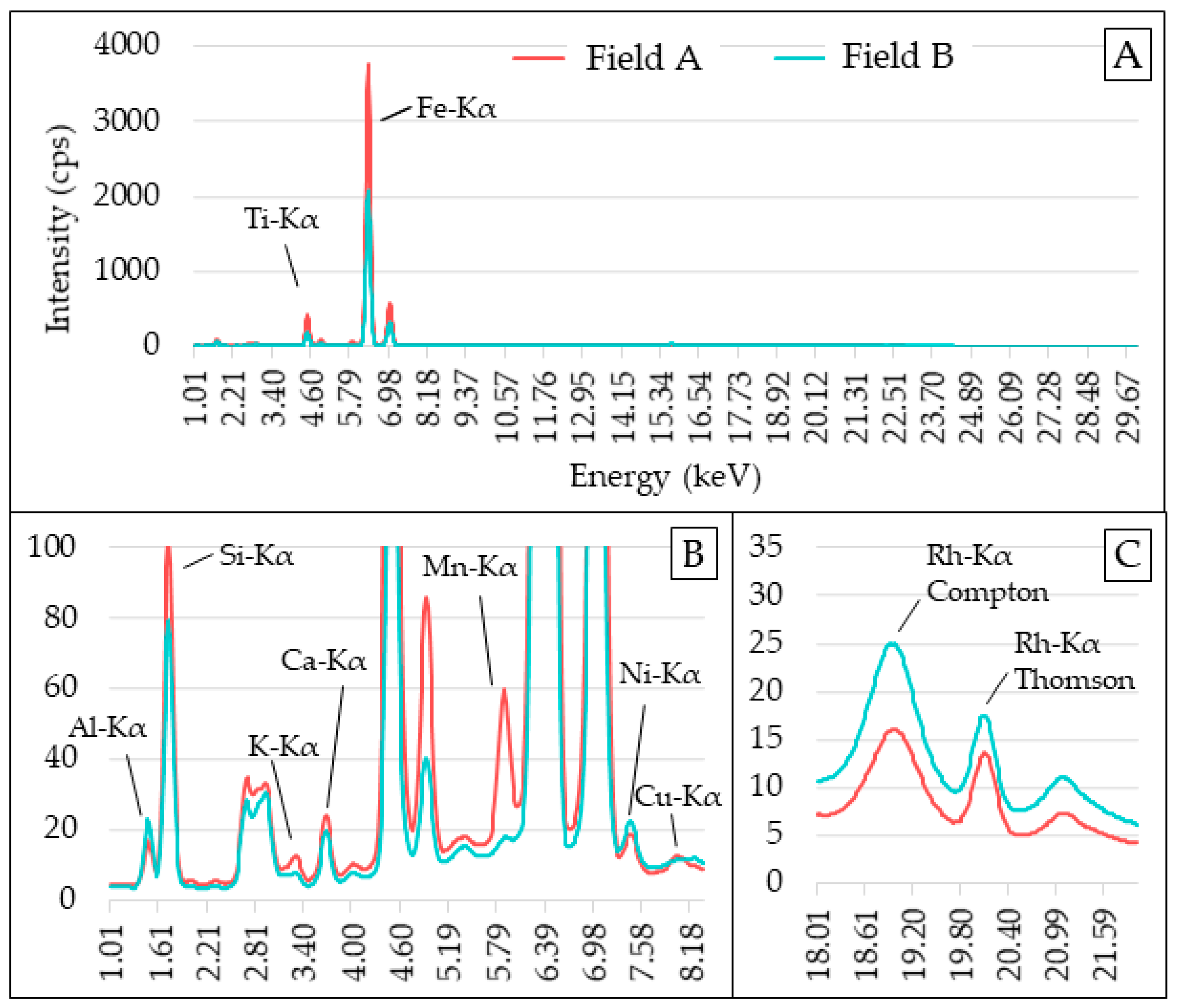
3.2. Exploratory Analysis of Texture Content and Spectral Data Obtained from Fields A and B

Figure 5 shows that the samples from Fields A and B had contrasting textural contents (clay and sand) and intensities of their vis–NIR spectra, which highlighted the presence of different matrices (i.e., different elemental and mineralogical compositions) in the dataset. Field A (represented in red in Figure 5) showed higher clay contents (ranging between 346 and 511 g dm−3) and lower sand contents (ranging between 233 and 334 g dm−3), while Field B (represented in blue in Figure 5) showed clay contents ranging between 175 and 328 g dm−3 and sand between 636 and 805 g dm−3. Different textural contents indicate different mineralogical and elemental composition [36]. The higher concentration of clay is related to the presence of Fe and Ti, which are components of clay minerals, such as hematite (α-Fe2O3) and goethite (FeOOH)—an isomorphic substitution of Fe for Ti eventually occurs in these minerals [37]. In turn, sandier soils tend to present a larger portion of Si in their composition in view of the presence of this element in quartz minerals (SiO2), commonly found in this fraction.
The behavior of the vis–NIR spectra of the Field A soils differed in intensity, shape, and features in relation to those of Field B (Figure 5B). This difference is also observed in the scores obtained via the principal component analysis; in its scatter plot (Figure 5C), it is possible to clearly identify two distinct groups, one with samples from Field A and the other with samples from only Field B. We emphasize that the first and second principal components explained more than 90% of the variance present in the spectra. The vis–NIR spectra of dry soil samples are primarily influenced by their grain size (i.e., related to soil texture) and mineralogical composition. Granulometry affects the reflectance intensity as a whole, with sandy soils showing a higher intensity than clayey soils [18,38]. This behavior is clearly observed in Figure 5B, where the soil reflectance intensity of Field B (in blue) is higher than that of Field A (in red). Regarding mineral features, the following were observed in the spectra of both areas: features of iron oxides and hydroxides (Fe–OH) around 900 nm and of hydroxyl groups (O-H) close to 1400 and 1900 nm, related to the structure of 1:1 and 2:1 minerals [18,39]. The main difference in the Field A and Field B absorption features was related to their intensity, with those in Field A being less pronounced than those in Field B. This, in turn, could be connected to either the lower concentration of these minerals in Field A, or to the attenuation of the absorption intensity of the Field A samples from the influence of other organic or mineralogical components (e.g., the presence of high levels of soil organic matter or opaque minerals can cause this attenuation) [40,41]. In summary, these results highlighted the ability of the vis–NIR spectrum to characterize the physical, mineralogical, and organic properties of the soil matrix.
Besides being noticed in the texture data and vis–NIR spectra, the differences in the elemental composition of the samples from the two study areas were also seen in the XRF spectra (Figure 2). The average emission intensities of the elements differed, in general, for all elements, with an emphasis on the Kα lines of Si, Ti, Fe, and Mn. Moreover, it is also noteworthy that the behavior of the scattering region (i.e., Rh-Kα Compton and Thomson) had an intensity directly proportional to the average atomic number of the sample [11]. It was observed that the sandier area (Field B) presented a higher intensity in the scattering region, which must be related to a lower presence of the elements Fe and Ti and a higher presence of Si in relation to Field A; Si has a lower atomic number than Fe and Ti which may have reduced the average atomic number of the Field B samples [42]. Thus, in the XRF spectra, both its elemental characterization and the intensity of the scattering region can be useful variables to characterize the matrix variations of soil samples.

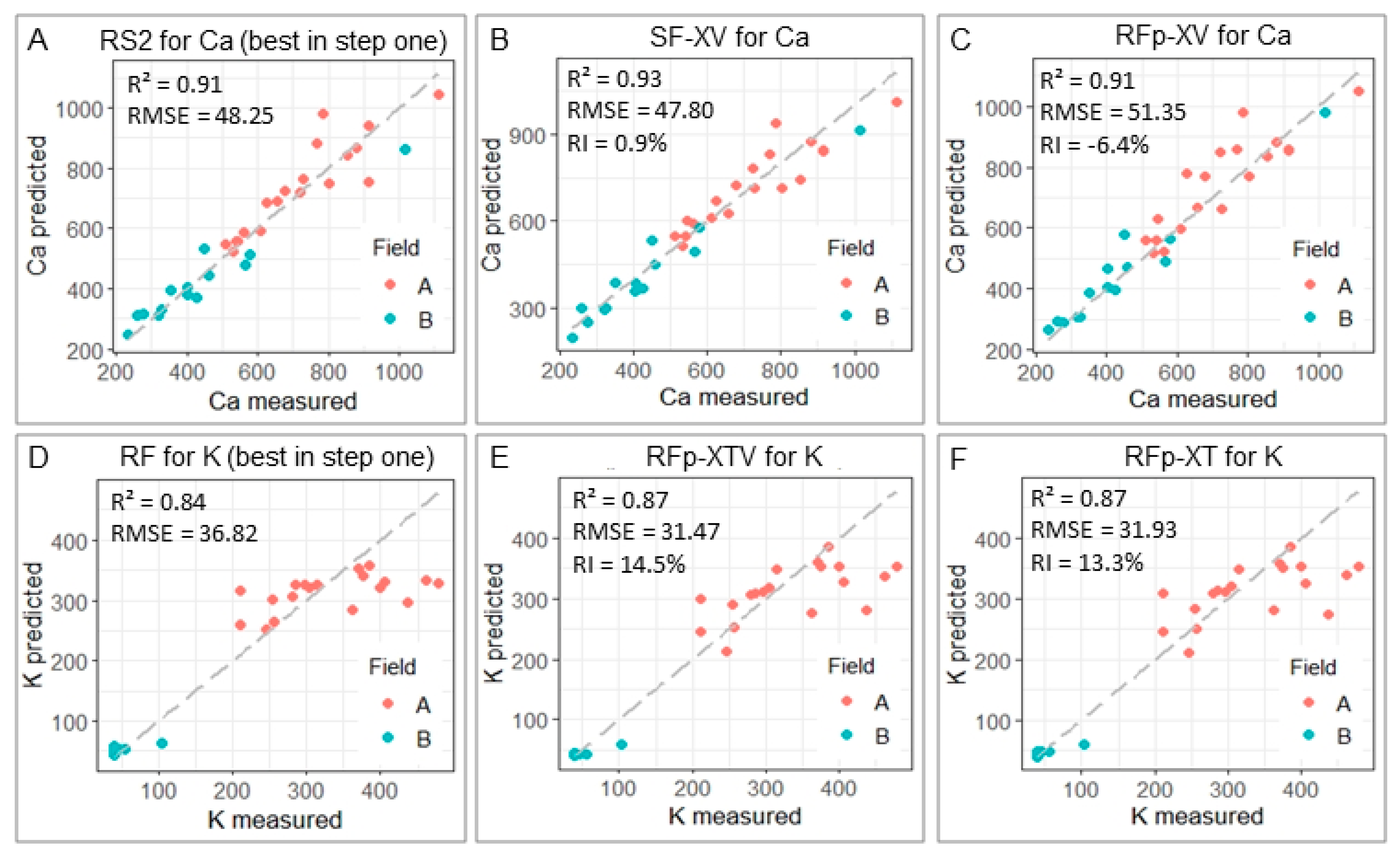
3.3. Ca and K Prediction Using XRF Data Associated with Different Modeling Strategies for Matrix Effect Mitigation (Data Modeling Step One)

The predictive performance for Ca and K achieved for the RS1, RS2, MLR, and PLS models are presented in Table 2. We observe that there was no sharp drop in performance when comparing the calibration and validation sets, which indicated no overfitting. The model that most diverged between calibration and validation was the RF, which reduced its R2 from 0.98 to 0.85 for Ca and from 0.98 to 0.84 for K. It is worth mentioning that PLS and RF methods depend on an optimal tuning of their parameters, and the proper choice of them is important to avoid under- or overfitting [12]. In the present study, well-defined criteria (described in Section 2.4) were used for the optimization of these parameters.
Table 2 shows that the worst prediction performance was obtained for model RS1, which presented in its validation the highest RMSE for both Ca (RMSE = 101.04 mg kg−1) and K (RMSE = 48.66 mg kg−1). It can also be seen that the RS1 models for Ca and K presented a dispersion of points more distant from the 1:1 line (Figure 6), indicating a performance degradation due to the matrix effect in this modeling strategy. This behavior is evident especially for Ca, which was more influenced than K by the matrix effect in this data set. This result was expected for the RS1 strategy since it did not consider any strategy for the matrix effect mitigation.
The matrix effect was mitigated when using all other models (RS2, MLR, PLS, and RF). In all of them, there was a performance gain over RS1, with an error reduction (on the validation set) ranging between 37.6 and 52.3% for Ca, and between 12.7 and 24.3% for K (Table 1). Visually, it was also noted that the points were closer to the 1:1 line with RS2, MLR, PLS, and RF when comparing their scatter plots to that of RS1 (Figure 5). The methods tested in step one showed the following increasing order of RMSE for the Ca prediction: RS2 < PLS < MLR < RF < RS1. For the K prediction, the order was RF < RS2 < MLR < PLS < RS1.
In this step one, the best validation performance was obtained for RS2 for the prediction of Ca (R2 = 0.92, RSME = 48.25 mg kg−1, and RI of 52.3%), and for RF for the prediction of K (R2 = 0.84, RSME = 36.82 mg kg−1, and RI of 24.3%). The second-best performance was obtained with the PLS strategy for Ca (R2 = 0.92, RSME = 51.68 mg kg−1, and RI of 48.8%) and with RS2 for K (R2 = 0.84, RSME = 39.62 mg kg−1, and RI of 18.6%). We emphasize that the best model for the Ca prediction was obtained by the most simplistic mitigation strategy, i.e., an association between a simple linear regression and a normalization of the Ca emission line by the Compton scattering. This result shows that complex models (e.g., computational modeling using an RF) do not always perform better than methods that use a linear fitting for soil attributes prediction via XRF data. The superior performance of traditional strategies over multivariate models was also observed by Aidene et al. [14], which evaluated both steel and ore samples via XRF. The mentioned authors observed that in general, a classical intensity-correction approach associated with a univariate linear regression (named IC by the authors) outperformed multivariate models. Nevertheless, the authors also pointed out that the multivariate models could provide satisfactory predictions. For example, nonlinear modeling using ANN and PLS outperformed the IC method for the Si prediction. On the other hand, the authors obtained quite similar results for the Mn prediction using both PLS and the IC strategy in ore samples. Similar to the work mentioned above, it was not possible to observe a single optimal approach for all attributes in our study. The best modeling approach in our study proved to be attribute-specific. The best prediction of K using a nonlinear model should be related to the lower SNR of K (Table A1), which leads to a greater interference of this signal by noise and, consequently, a greater complexity of its relationship with the concentration of this element in the soil.
The amount and complexity of information present in an XRF spectrum of soil samples leads one to expect that nonlinear models may be the best alternative for the calibration of predictive models for predicting its attributes. However, the data from the present study showed that this was not always true, since although K obtained the best predictive performance with RF, Ca was better predicted using the RS2 strategy. The literature also reports this divergence. On the one hand, univariate approaches obtained superior results for the highest attributes in the study conducted by Aidene et al. [14]. On the other, the opposite was observed by Facchin et al. [15], who obtained the best performance when using nonlinear methods (artificial neural network model) for the determination of sulfur in synthetic samples. By using this nonlinear model, the authors obtained an error reduction of 59% for Pb determination and 80% for S determination, when comparing the performance with univariate linear models. In turn, when using a PLS model, the authors noticed an error reduction of 23% for Pb determination and 62% for S. So far, these results indicate the need to test different models in order to optimize the modeling strategy for the dataset at hand. It is worth mentioning that possibly, nonlinear models will have advantages in larger databases (e.g., n > 500), with larger varieties of soil types, and further studies are needed in this scenario. Finally, we mention that the construction of reliable multivariate models requires a significant number of calibration and validation samples with known target parameters. This may pose a problem since these samples can be expensive and hardly available for particular applications [12].
In summary, our results obtained in the data modeling step one showed that complex models (e.g., computational modeling using RF) do not always perform better than methods that use linear fitting for soil attributes’ prediction via XRF data. This occurred because the best Ca prediction performance was obtained with a simple linear regression using the Ca emission line normalized by the Compton peak (i.e., a classical matrix-effect mitigation strategy). On the other hand, the prediction of K performed optimally when using an RF computer model, which makes it possible to suggest such approach for this specific attribute.

3.4. Prediction of Ca and K Using XRF Data Associated with Texture and vis–NIR Spectra as Auxiliary Information (Data Modeling Step Two)

Table 3 shows the predictive performance of the models using soil texture data and vis–NIR spectra as auxiliary variables and, through the RI value, compares the performance of each one with the one obtained by the best approach of step one. For Ca prediction, it was observed that only the SF-XV model (which used both XRF and vis–NIR spectral data) outperformed RS2, presenting an R2 of 0.93 and RMSE of 47.80 mg kg−1 (Table 3). The improvement was subtle, with an RI of 0.9% (Figure 5), suggesting that the tradeoff of this performance gain should be weighed against the extra work to obtain the vis–NIR data to decide whether to use this strategy or not.
Figure 7 compares the two best strategies of step two with the best strategy of step one. It was noted that the K predictions that used data fusion presented a higher RI than the Ca predictions. The K predictions yielded RI > 10% and the only Ca prediction that presented a performance gain (SF-XV) reached an RI of 0.9%. Therefore, in this study the use of auxiliary variables may be a promising alternative to increase the analytical performance of the determination of K in soils, with a performance gain of up to 14.5% (for RFp-XTV). Interestingly, for the prediction of K, the data fusion strategies that outperformed the best model from step one (i.e., RF) were the strategies that used the prediction as input for the model calibration (RFp-XT, RFp-XV, and RFp-XTV). That is, none of the models that used the entire XRF spectrum together with auxiliary information (SF-XT, SF-XV, and SF-XTV) showed any performance gain compared to the RF strategy (Table 3). These results show that the way of imputing the XRF information is important when defining the data fusion method to be used. Strategies that use the spectra associated with auxiliary information are considered front-end approaches, i.e., fusion methods that use all available information, by integrating the entire data of different sources as inputs for the model calibration [43,44]. Conversely, back-end approaches, such as RFp-XT, RFp-XV, and RFp-XTV, may not take advantage of all the information provided by multiple sources, which can be considered a drawback [17]. However, this behavior was not observed in the present study. Comparable results, with similar or better performance for back-end versus front-end approaches, have also been reported by other authors [44,45].
An extra challenge regarding using auxiliary data for matrix effect mitigation is standardizing this information for model calibration and extrapolation. For example, soil texture data are obtained by traditional laboratory analysis, which can be error-prone if the procedure is not rigorously followed [4]. Similarly, vis–NIR spectra need to have standard instrumental conditions, instrument calibration, and data acquisition geometry. Otherwise, they produce nonreplicable models [46].
Briefly, the results obtained in the data modeling step two showed modest performance gains for the Ca prediction when using auxiliary variables, which may not justify the extra effort to implement this data fusion strategy for this attribute. On the other hand, the K prediction showed performance gains of up to 14.5% when using a vis–NIR sensor and/or textural data as auxiliary variables. This research provides a step towards understanding the relationships between the attributes of tropical soils and data from XRF and vis–NIR sensors. Further research needs to involve larger databases, with more complex matrix effects, different soil types, a wider range of nutrient contents, as well as other strategies of data modeling (e.g., spectra fusion). This knowledge is fundamental for the development of modeling strategies that will compose the sensor intelligence in analytical methods that are faster, more practical, and in accordance with the precepts of green chemistry.

4. Conclusions

This paper presented a comparative analysis of a wide range of strategies for matrix effect mitigation in soil analysis with XRF, comparing the association of XRF data with traditional and multivariate methods and their fusion with auxiliary data. The results showed that it was possible to mitigate the matrix effect in soil samples with a reasonable dissimilarity of chemical composition, enabling the determination of their Ca and K contents with excellent predictive performance (R2 ≥ 0.84).
The optimal predictive strategy reached for each attribute differed from one another, and it was not possible to find a single optimal method. The best performance was obtained with a simple regression associated with a Compton normalization (RS2), for the prediction of Ca (with R2 = 0.92), and with random forest (RF) models using the full XRF spectra, for the prediction of K (with R2 = 0.84). The results indicated that complex models (e.g., computational modeling using RF) did not always perform better than those using linear fitting to predict soil attributes via XRF data.
Regarding auxiliary data, it was observed that the predictive models for Ca did not show significant gains when including information from soil texture and/or vis–NIR spectra. For the Ca prediction, the RFp-XV approach, i.e., with spectral data from XRF and vis–NIR sensors, was the only one to show a performance gain over RS2 (best strategy without using auxiliary data), but only with a subtle gain of 0.9%. On the other hand, the predictions of K that used back-end approaches (RFp-XT, RFp-XV, and RFp-XTV) showed RI greater than 10%, suggesting that for this attribute the use of auxiliary variables can be a promising alternative to increase the analytical performance of its determination via XRF.
The results of the present study together with the lack of consensus in the literature regarding a single optimal method for matrix effect mitigation in soil samples suggest that the optimal approach for matrix effect mitigation depends on the complexity of the soil matrix effect involved in a particular dataset. Hence, it might be database-specific. Research involving datasets with larger sample sizes (e.g., spectral libraries) and new modeling strategies should be further addressed.

Author Contributions

Conceptualization, T.R.T., E.d.A. and H.W.P.d.C.; methodology, T.R.T. and A.G.; validation, E.d.A., C.R.P.J. and P.R.F.; formal analysis, T.R.T. and C.R.P.J.; investigation, T.R.T.; resources, T.R.T. and H.W.P.d.C.; data curation, T.R.T. and A.G.; writing—original draft preparation, T.R.T. and P.R.F.; writing—review and editing, E.d.A., A.G., C.R.P.J. and H.W.P.d.C.; visualization, E.d.A. and H.W.P.d.C.; supervision, H.W.P.d.C.; project administration, T.R.T.; funding acquisition, T.R.T. and H.W.P.d.C. All authors have read and agreed to the published version of the manuscript.

Funding

T.R.T. was funded by São Paulo Research Foundation (FAPESP), grant number 2020/16670-9. We also thank the research productivity fellowship from the Brazilian National Council for Scientific and Technological Development (CNPq) (grant number 306185/2020-2). XRF facilities were funded by FAPESP, grant number 2015-19121-8, and “Financiadora de Estudos e Projetos” (FINEP) project “Core Facility de suportes às pesquisas em Nutrologia e Segurança Alimentar na USP”, grant number 01.12.0535.0.

Data Availability Statement

Data can be provided by the corresponding authors upon request.

Conflicts of Interest

The authors declare no conflict of interest.

Appendix A

Table A1 shows the signal-to-noise ratio (SNR), which was determined by dividing the characteristic X-ray net intensities by the background square root [47].
Table A1. Descriptive statistics of signal-to-noise ratio (SNR) obtained for Al, Si, K, Ca, Ti, Mn, Fe, Ni, and Cu K-lines.
Al-KαSi-KαK-KαCa-KαTi-KαMn-KαFe-KαNi-KαCu-Kα
Min7.2348.030.556.7586.651.50886.764.251.04
1Quart8.2759.371.419.72119.732.141082.564.821.61
media10.9063.532.4912.30182.4212.121426.265.772.79
3Quart14.2967.593.4414.04237.6620.151702.616.853.70
Max15.9780.474.6324.95256.0122.591781.728.114.13

References

  1. Weindorf, D.C.; Chakraborty, S. Portable X-ray fluorescence spectrometry analysis of soils. Soil Sci. Soc. Am. J. 2020, 84, 1384–1392. [Google Scholar] [CrossRef]
  2. Gredilla, A.; Fdez-Ortiz de Vallejuelo, S.; Elejoste, N.; de Diego, A.; Madariaga, J.M. Non-destructive Spectroscopy combined with chemometrics as a tool for Green Chemical Analysis of environmental samples: A review. TrAC Trends Anal. Chem. 2016, 76, 30–39. [Google Scholar] [CrossRef]
  3. Marguí, E.; Queralt, I.; de Almeida, E. X-ray fluorescence spectrometry for environmental analysis: Basic principles, instrumentation, applications and recent trends. Chemosphere 2022, 303, 135006. [Google Scholar] [CrossRef] [PubMed]
  4. Viscarra Rossel, R.A.; Bouma, J. Soil sensing: A new paradigm for agriculture. Agric. Syst. 2016, 148, 71–74. [Google Scholar] [CrossRef]
  5. Van Raij, B.; Andrade, J.C.; Cantarela, H.; Quaggio, J.A. Análise Química Para Avaliação De Solos Tropicais; IAC: Campinas, Brazil, 2001.
  6. Kuang, B.; Mahmood, H.S.; Quraishi, M.Z.; Hoogmoed, W.B.; Mouazen, A.M.; van Henten, E.J. Sensing Soil Properties in the Laboratory, In Situ, and On-Line. Adv. Agron. 2012, 114, 155–223. [Google Scholar] [CrossRef]
  7. Viscarra Rossel, R.A.; Adamchuk, V.I.; Sudduth, K.A.; McKenzie, N.J.; Lobsey, C. Proximal Soil Sensing: An Effective Approach for Soil Measurements in Space and Time. Adv. Agron. 2011, 113, 243–291. [Google Scholar] [CrossRef]
  8. Bowers, C. Matrix Effect Corrections in X-ray Fluorescence Spectrometry. J. Chem. Educ. 2019, 96, 2597–2599. [Google Scholar] [CrossRef]
  9. Protection, U.-U.S.E. Method 6200: Field Portable X-ray Fluorescence Spectrometry for the Determination of Elemental Concentrations in Soil and Sediment; USA Environmental Protection Agency: Washington, DC, USA, 2007.
  10. Kalnicky, D.J.; Singhvi, R. Field portable XRF analysis of environmental samples. J. Hazard. Mater. 2001, 83, 93–122. [Google Scholar] [CrossRef] [Green Version]
  11. Yılmaz, D.; Boydaş, E. The use of scattering peaks for matrix effect correction in WDXRF analysis. Radiat. Phys. Chem. 2018, 153, 17–20. [Google Scholar] [CrossRef]
  12. Panchuk, V.; Yaroshenko, I.; Legin, A.; Semenov, V.; Kirsanov, D. Application of chemometric methods to XRF-data—A tutorial review. Anal. Chim. Acta 2018, 1040, 19–32. [Google Scholar] [CrossRef]
  13. Braga, J.W.B.; Trevizan, L.C.; Nunes, L.C.; Rufini, I.A.; Santos, D.; Krug, F.J. Comparison of univariate and multivariate calibration for the determination of micronutrients in pellets of plant materials by laser induced breakdown spectrometry. Spectrochim. Acta Part B At. Spectrosc. 2010, 65, 66–74. [Google Scholar] [CrossRef]
  14. Aidene, S.; Khaydukova, M.; Pashkova, G.; Chubarov, V.; Savinov, S.; Semenov, V.; Kirsanov, D.; Panchuk, V. Does chemometrics work for matrix effects correction in X-ray fluorescence analysis? Spectrochim. Acta Part B At. Spectrosc. 2021, 185, 106310. [Google Scholar] [CrossRef]
  15. Facchin, I.; Mello, C.; Bueno, M.I.M.S.; Poppi, R.J. Simultaneous determination of lead and sulfur by energy-dispersive x-ray spectrometry. Comparison between artificial neural networks and other multivariate calibration methods. X-Ray Spectrom. 1999, 28, 173–177. [Google Scholar] [CrossRef]
  16. Sharma, A.; Weindorf, D.C.; Wang, D.; Chakraborty, S. Characterizing soils via portable X-ray fluorescence spectrometer: 4. Cation exchange capacity (CEC). Geoderma 2015, 239–240, 130–134. [Google Scholar] [CrossRef]
  17. Tavares, T.R.; Molin, J.P.; Hamed Javadi, S.; de Carvalho, H.W.P.; Mouazen, A.M. Combined use of vis-nir and xrf sensors for tropical soil fertility analysis: Assessing different data fusion approaches. Sensors 2021, 21, 148. [Google Scholar] [CrossRef] [PubMed]
  18. Nocita, M.; Stevens, A.; van Wesemael, B.; Aitkenhead, M.; Bachmann, M.; Barthès, B.; Ben Dor, E.; Brown, D.J.; Clairotte, M.; Csorba, A.; et al. Soil Spectroscopy: An Alternative to Wet Chemistry for Soil Monitoring. Adv. Agron. 2015, 132, 139–159. [Google Scholar] [CrossRef]
  19. Stenberg, B.; Viscarra Rossel, R.A.; Mouazen, A.M.; Wetterlind, J. Visible and Near Infrared Spectroscopy in Soil Science. Adv. Agron. 2010, 107, 163–215. [Google Scholar] [CrossRef] [Green Version]
  20. IUSS Working Group WRB. World Reference Base for Soil Resources 2014, Update 2015: International Soil Classification System for Naming Soils and Creating Legends for Soil Maps; Schad, P., van Huyssteen, C., Micheli, E., Eds.; FAO: Rome, Italy, 2015; ISBN 978-92-5-108369-7. [Google Scholar]
  21. Element, C.A.S. Method 3051A microwave assisted acid digestion of sediments, sludges, soils, and oils. Z.Für Anal.Chem 2007, 111, 362–366. [Google Scholar]
  22. Bouyoucos, G.J. A Recalibration of the Hydrometer Method for Making Mechanical Analysis of Soils 1. Agron. J. 1951, 43, 434–438. [Google Scholar] [CrossRef] [Green Version]
  23. Tavares, T.R.; Molin, J.P.; Nunes, L.C.; Alves, E.E.N.; Melquiades, F.L.; de Carvalho, H.W.P.; Mouazen, A.M.; de Carvalho, H.W.P.; Mouazen, A.M. Effect of X-Ray Tube Configuration on Measurement of Key Soil Fertility Attributes with XRF. Remote Sens. 2020, 12, 963. [Google Scholar] [CrossRef] [Green Version]
  24. Christy, C.; Drummond, P. Mobile Soil Mapping System for Collecting Soil Reflectance Measurements 2012. U.S. Patent No. 8,204,689, 19 June 2012. [Google Scholar]
  25. Kennard, R.W.; Stone, L.A. Computer Aided Design of Experiments. Technometrics 1969, 11, 137–148. [Google Scholar] [CrossRef]
  26. Kokaly, R. Spectroscopic Determination of Leaf Biochemistry Using Band-Depth Analysis of Absorption Features and Stepwise Multiple Linear Regression. Remote Sens. Environ. 1999, 67, 267–287. [Google Scholar] [CrossRef]
  27. Tavares, T.R.; Mouazen, A.M.; Alves, E.E.N.; Dos Santos, F.R.; Melquiades, F.L.; De Carvalho, H.W.P.; Molin, J.P. Assessing soil key fertility attributes using a portable X-ray fluorescence: A simple method to overcome matrix effect. Agronomy 2020, 10, 787. [Google Scholar] [CrossRef]
  28. Nawar, S.; Mouazen, A. Comparison between Random Forests, Artificial Neural Networks and Gradient Boosted Machines Methods of On-Line Vis-NIR Spectroscopy Measurements of Soil Total Nitrogen and Total Carbon. Sensors 2017, 17, 2428. [Google Scholar] [CrossRef]
  29. Breiman, L. Random forests. Mach. Learn. 2001, 45, 5–32. [Google Scholar] [CrossRef] [Green Version]
  30. Guio Blanco, C.M.; Brito Gomez, V.M.; Crespo, P.; Ließ, M. Spatial prediction of soil water retention in a Páramo landscape: Methodological insight into machine learning using random forest. Geoderma 2018, 316, 100–114. [Google Scholar] [CrossRef]
  31. Strobl, C.; Boulesteix, A.-L.; Kneib, T.; Augustin, T.; Zeileis, A. Conditional variable importance for random forests. BMC Bioinform. 2008, 9, 307. [Google Scholar] [CrossRef] [Green Version]
  32. Bellon-Maurel, V.; Fernandez-Ahumada, E.; Palagos, B.; Roger, J.-M.; McBratney, A. Critical review of chemometric indicators commonly used for assessing the quality of the prediction of soil attributes by NIR spectroscopy. TrAC Trends Anal. Chem. 2010, 29, 1073–1081. [Google Scholar] [CrossRef]
  33. Nawar, S.; Mouazen, A.M. Predictive performance of mobile vis-near infrared spectroscopy for key soil properties at different geographical scales by using spiking and data mining techniques. CATENA 2017, 151, 118–129. [Google Scholar] [CrossRef] [Green Version]
  34. Nawar, S.; Mouazen, A.M. Optimal sample selection for measurement of soil organic carbon using on-line vis-NIR spectroscopy. Comput. Electron. Agric. 2018, 151, 469–477. [Google Scholar] [CrossRef]
  35. Letey, J. Relationship between Soil Physical Properties and Crop Production. In Advances in Soil Science; Stewart, B.A., Ed.; Springer: New York, NY, USA, 1958; pp. 277–294. ISBN 978-1-4612-5046-3. [Google Scholar]
  36. Schäefer, C.E.G.R.; Fabris, J.D.; Ker, J.C. Minerals in the clay fraction of Brazilian Latosols (Oxisols): A review. Clay Miner. 2008, 43, 137–154. [Google Scholar] [CrossRef]
  37. Singh, B.; Gilkes, R.J. Properties and distribution of iron oxides and their association with minor elements in the soils of south-western Australia. J. Soil Sci. 1992, 43, 77–98. [Google Scholar] [CrossRef]
  38. Ben-Dor, E. Quantitative remote sensing of soil properties. Adv. Agron. 2002, 75, 173–243. [Google Scholar] [CrossRef]
  39. Terra, F.S.; Demattê, J.A.M.; Viscarra Rossel, R.A. Spectral libraries for quantitative analyses of tropical Brazilian soils: Comparing vis–NIR and mid-IR reflectance data. Geoderma 2015, 255–256, 81–93. [Google Scholar] [CrossRef]
  40. Demattê, J.A.; Campos, R.C.; Alves, M.C.; Fiorio, P.R.; Nanni, M.R. Visible–NIR reflectance: A new approach on soil evaluation. Geoderma 2004, 121, 95–112. [Google Scholar] [CrossRef]
  41. Bellinaso, H.; Demattê, J.A.M.; Romeiro, S.A. Soil spectral library and its use in soil classification. Rev. Bras. Ciência Do Solo 2010, 34, 861–870. [Google Scholar] [CrossRef] [Green Version]
  42. Lu, J.; Guo, J.; Wei, Q.; Tang, X.; Lan, T.; Hou, Y.; Zhao, X. A Matrix Effect Correction Method for Portable X-ray Fluorescence Data. Appl. Sci. 2022, 12, 568. [Google Scholar] [CrossRef]
  43. Zhang, Y.; Hartemink, A.E. Data fusion of vis–NIR and PXRF spectra to predict soil physical and chemical properties. Eur. J. Soil Sci. 2020, 71, 316–333. [Google Scholar] [CrossRef]
  44. Xu, D.; Chen, S.; Viscarra Rossel, R.A.; Biswas, A.; Li, S.; Zhou, Y.; Shi, Z. X-ray fluorescence and visible near infrared sensor fusion for predicting soil chromium content. Geoderma 2019, 352, 61–69. [Google Scholar] [CrossRef]
  45. O’Rourke, S.M.; Stockmann, U.; Holden, N.M.; McBratney, A.B.; Minasny, B. An assessment of model averaging to improve predictive power of portable vis-NIR and XRF for the determination of agronomic soil properties. Geoderma 2016, 279, 31–44. [Google Scholar] [CrossRef]
  46. Da Silveira Paiva, A.F.; Poppiel, R.R.; Rosin, N.A.; Greschuk, L.T.; Rosas, J.T.F.; Demattê, J.A.M. The Brazilian Program of soil analysis via spectroscopy (ProBASE): Combining spectroscopy and wet laboratories to understand new technologies. Geoderma 2022, 421, 115905. [Google Scholar] [CrossRef]
  47. Ernst, T.; Berman, T.; Buscaglia, J.; Eckert-Lumsdon, T.; Hanlon, C.; Olsson, K.; Palenik, C.; Ryland, S.; Trejos, T.; Valadez, M.; et al. Signal-to-noise ratios in forensic glass analysis by micro X-ray fluorescence spectrometry. X-Ray Spectrom. 2014, 43, 13–21. [Google Scholar] [CrossRef]
Figure 1. Framework of the methodology applied for assessing the optimal predictive strategy to analyze Ca and K contents, via X-ray fluorescence spectroscopy (XRF), in a sample set of tropical soils with contrasting matrices. Sand and clay content of samples (texture) and data acquired with visible and near-infrared diffuse reflectance spectroscopy (vis–NIR) were evaluated as auxiliary variables. The strategies evaluated in step one of the data modeling were: a simple linear regression using the emission line of the element of interest without (RS1) and with Compton normalization (RS2); a multiple linear regression with a stepwise procedure using selected emission lines (MLR); partial least-squares regression (PLS) and random forest (RF) models using the entire XRF spectrum.
Agriengineering 05 00043 g001
Figure 2. Mean XRF spectra of Fields A and B (A). Snapshot of the emission lines from 1.00 to 8.20 keV (B) and scattering peaks (C). XRF spectra intensities are shown in counts of photons per second (cps).
Agriengineering 05 00043 g002
Figure 3. Methodology framework applied for conducting steps one and two of data modeling. * In the strategies of step two that used the XRF prediction, the result of the K or Ca prediction that had the best performance in step one was used.
Agriengineering 05 00043 g003
Figure 4. Boxplots of Ca and K contents for the calibration (CAL) and validation (VAL) sets (upper part, (A,B)) and for Fields A and B (shown at the bottom, (C,D)).
Agriengineering 05 00043 g004
Figure 5. Boxplots of clay and sand contents for Fields A and B (A), raw vis–NIR spectra from Fields A and B (B), and scores of principal components 1 and 2 obtained after applying a principal component analysis on the vis–NIR spectra (C). The information of Field A is presented in red and Field B in blue.
Agriengineering 05 00043 g005
Figure 6. Scatter plots comparing predicted and measured Ca (AE) and K (FJ) values (for the validation dataset, n = 30) obtained with the modeling strategies RS1, RS2, MLR, PLS, and RF. The coefficient of determination (R2) and root-mean-square error (RMSE) are also presented.
Agriengineering 05 00043 g006
Figure 7. Scatter plots comparing the predicted and measured Ca and K values (for the validation dataset, n = 30) for the best strategy of step one that involved only data from the XRF sensor (A,D) and for the two best models of step two (B,C,E,F) that used auxiliary variables.
Agriengineering 05 00043 g007
Table 1. Result of the optimization of the mtry parameter, which was applied to calibrate the models involving RF.
RF for CaRF for KSF-XT for KSF-XV for KSF-XTV for KRFp-XT for CaRFp-XV for CaRFp-XTV for CaRFp-XT for KRFp-XV for KRFp-XTV for K
798652123612361090346346
Table 2. Prediction performance for Ca and K, for the calibration and validation sets, obtained using the modeling strategies RS1, RS2, MLR, PLS, and RF.
R2RMSERMSE%RPIQRI * R2RMSERMSE%RPIQRI *
calibration set—Cacalibration set—K
RS10.67112.2717.983.48RS10.8539.5419.816.93
RS20.9341.656.679.3762.9RS20.8933.7516.928.1214.6
MLR0.9246.957.528.3158.2MLR0.9129.7514.919.2124.7
PLS0.9538.606.1810.1165.6PLS0.9720.8810.4613.1347.2
RF0.9821.913.5117.8080.5RF0.9814.297.1619.1863.8
validation set—Cavalidation set—K
RS10.73101.0416.833.39RS10.7848.6623.046.62
RS20.9148.258.047.1052.3RS20.8439.6218.768.1318.6
MLR0.9253.358.896.4247.2MLR0.8140.5319.197.9516.7
PLS0.9251.688.616.6348.8PLS0.8342.5120.127.5812.7
RF0.8563.0910.515.4337.6RF0.8436.8217.438.7524.3
The values of the root-mean-square error (RMSE) and the ratio of performance to interquartile range (RPIQ) are presented in a gray scale, highlighting the lowest values for the RMSE and the highest values for the RPIQ. The RMSE is presented in mg kg−1 for Ca and K. * The relative improvement (RI) of the model validation was calculated by comparing with the RMSE of the best performing strategy from step 1 (RS2 for Ca and RF for K); RI shows the reduction (when positive) or increase (when negative) of the RMSE in percent.
Table 3. Ca and K prediction performance, for calibration and validation datasets, obtained for modeling strategies of step two that use auxiliary data.
R2RMSERMSE%RPIQRI * R2RMSERMSE%RPIQRI *
Calibration dataset—CaCalibration dataset—K
SF 1-XT0.9537.085.9410.52SF 2-XT0.9814.077.0519.49
SF 1-XV0.9541.236.69.46SF 2-XV0.9813.746.8919.94
SF 1-XTV0.9538.356.1410.17SF 2-XTV0.9814.267.1519.23
RFp-XT0.9819.963.219.54RFp-XT0.994.432.2261.81
RFp-XV0.9819.743.1619.76RFp-XV0.994.552.2860.25
RFp-XTV0.9818.652.9920.91RFp-XTV0.994.442.2261.77
Validation dataset—CaValidation dataset—K
SF 1-XT0.9158.459.745.86−21.1SF 2-XT0.8437.1517.598.67−0.9
SF 1-XV0.9347.87.967.160.9SF 2-XV0.8536.917.478.73−0.2
SF 1-XTV0.9252.38.716.55−8.4SF 2-XTV0.8437.9217.958.49−3.00
RFp-XT0.9152.638.776.51−9.1RFp-XT0.8731.9315.1210.0913.3
RFp-XV0.9151.358.566.67−6.4RFp-XV0.8732.7515.59.8311.1
RFp-XTV0.9152.978.826.47−9.8RFp-XTV0.8731.4714.910.2314.5
1 Data fusion strategy that used PLS for modeling. 2 Data fusion strategy that used RF for modeling. The values of the root-mean-square error (RMSE) and the ratio of performance to interquartile range (RPIQ) are presented in gray scale, highlighting the lowest values for the RMSE and the highest values for the RPIQ. The RMSE is presented in mg kg−1 for Ca and K. * The relative improvement (RI) of the model validation was calculated by comparing with the RMSE of the best performing strategy from step 1 (RS2 for Ca and RF for K); RI shows the reduction (when positive) or increase (when negative) of the RMSE in percent.
Disclaimer/Publisher’s Note: The statements, opinions and data contained in all publications are solely those of the individual author(s) and contributor(s) and not of MDPI and/or the editor(s). MDPI and/or the editor(s) disclaim responsibility for any injury to people or property resulting from any ideas, methods, instructions or products referred to in the content.

