Article

In-Season Wheat Yield Forecasting at High Resolution Using Regional Climate Model and Crop Model

Indian Institute of Remote Sensing (ISRO), Dehradun 248 001, Uttrakhand, India
*
Author to whom correspondence should be addressed.
AgriEngineering 2022, 4(4), 1054-1075; https://doi.org/10.3390/agriengineering4040066
Submission received: 1 October 2022 / Revised: 17 October 2022 / Accepted: 20 October 2022 / Published: 30 October 2022
(This article belongs to the Special Issue Agrometeorology Tools and Applications for Precision Farming)

Abstract

:
In-season crop production forecasts at the regional or sub-regional scale are essential to aid in food security through early warning of harvest shortfall/surplus, tailoring crop management decisions and addressing climatic shock. Considering the efforts to establish a framework towards quantifying the crop yield prediction at regional scales are limited, we investigated the utility of combining crop model with the regional weather prediction model to forecast winter wheat yields over space. The exercise was performed for various lead-times in the regions of Punjab and Haryana for the years 2008–2009. A numerical weather prediction (NWP) model was used to generate micro-meteorological variables at different lead times (1-week, 2-weeks, 3-weeks and 5-weeks) ahead of crop harvest and used within the CERES-Wheat crop simulation model gridded framework at a spatial resolution of 10 km. Various scenarios of the yield forecasts were verified with district-wide reported yield values. Average deviations of −12 to 3% from the actual district-wise wheat yields were observed across the lead times. The 3-weeks-ahead yield forecasts yielded a maximum agreement index of 0.86 with a root mean squared error (RMSE) of 327.75 kg/ha and a relative deviation of −5.35%. The critical crop growth stages were found to be highly sensitive to the errors in the weather forecast, and thus made a huge impact on the predicted crop yields. The 5-weeks-ahead weather forecasts generated anomalous meteorological data during flowering and grain-filling crop growth stages, and thus had the highest negative impact on the simulated yields. The agreement index of the 5-week-ahead forecasts was 0.41 with an RMSE of 415.15 kg ha−1 and relative deviation of −2.77 ± 5.01. The proposed methodology showed significant forecast skill for extended space and time scale crop yield forecasting, offering scope for further research and practical applicability.

1. Introduction

Wheat is one of the major food crops and contributes to about 30% of cereal production globally. India is the second largest producer of global wheat and wheat is the second most important food crop in the country [1]. About 94% of the wheat in India is grown under irrigated conditions with gross areal coverage of 30 million hectares, representing a production of 99.7 million tonnes and average productivity of about 3371 kg/ha [2]. Wheat in India is typically grown in dry winter–spring season, also known as rabi season extending from November to April. The wheat yield can be analysed from two components viz. grains per square meters and weight per kernel. Both of the components are strongly controlled by radiation and temperature when water and nutrient availability are not constrained [3].
Forecasting food grain yield in developing countries is an important aspect of agricultural management, food security warning and food trade policy [4,5,6]. Crop yield forecasting spans across spatial and temporal scales with several approaches viz. empirical, semi-empirical and physical based methods. Given that the weather is very critical in the assessment of wheat yield, approaches which address the weather-crop interaction are explicitly required. Crop simulation models, which account for the interactions between weather, crop, soil, management and their effect on crop yield, are widely used to develop process-based methodologies rather than regression-based approaches [7]. In particular, in developing countries, such as India, where long historical records on the crop details are not available, process-based approaches are quite helpful. One of the major challenges in the process-based approach is the uncertainty associated with the unknown weather in the future time scales [7]. Studies have attempted to use seasonal outlooks (typically having grid sizes >50 km) available from global numerical weather prediction (NWP) models [8,9,10,11] to predict regional crop productions, mainly for regions with sparsely distributed weather observatories.
In the tropics and sub-tropics, the region-specific circulations and local feedbacks generated by strong soil-plant-atmosphere coupling induces variability to the large-scale phenomenon predicted by the coarser resolution global NWP models [12]. Thus, the season-long outlooks might fail to capture the variances and occurrences of extreme events at daily time step [13,14], hugely limiting the applicability in crop growth models. The spatio-temporal uncertainties in the simulated weather parameters during season-long predictions can be reduced with medium-range forecasts [15]. Ortiz-Monasterio et al. [3], after analysing winter wheat from 1985–1992 in the district of Punjab, India, suggested that high temperatures about and after the heading date (which occurred during the middle of February) had a detrimental effect on the crop yield. Lobell et al. [16] specifically addressed the extreme heat effects on Indian wheat and reported that a 2 °C increase in temperature during the grain filling stage (post heading date) reduced the simulated yield by 50% in the crop models. Several other studies [17,18,19] have also concluded that the heat stress, particularly during the grain filling stage, had a negative impact on the wheat yield. Accordingly, the weather events in the post-heading days (towards the end of the growing season) are a precursor to the Indian winter wheat yield assessment.
As a result, high-resolution medium-extended (10–30 days) range (sub-seasonal scale) weather forecasts can be very appropriate and cost-effective in acquiring real-time accurate in-season estimates of wheat yield, when compared to full-season predictions. Bannayan et al. [20] tested the performance of a crop simulation model (CERES-Wheat) to forecast within-season wheat yields across the United Kingdom. They used synthetically generated weather forecasts from a weather generator for the forecast period, which started at different growth stages of wheat viz. leaf senescence, 150 days after sowing, flag leaf appearance, heading and milking stages. The forecast period set at the milking stage (towards the end of the season) provided considerable advantage over the other forecast scenarios reducing the root mean squared difference in the estimated yield. Marletto et al. [21] used the downscaled weather forecasts for the last two months before harvest to examine the skill of NWP models in early wheat yield assessments across Italy. They concluded that wheat yields showed reasonable predictability (r-squared of 0.65) two months before harvest and gave comparable yield estimates with those simulated with actual weather data. Zhuo et al. [22] used a 15-day THORPEX Interactive Grand Global Ensemble (TIGGE) forecast dataset and concluded that combining TIGGE and historical weather data helped in medium- and short-term winter wheat yield forecasting.
The major research gap found in general among within-season crop forecasting was the point-scale setup of the crop simulation model, which failed to address the spatial variability. The major challenge in spatial crop modeling is the availability of high-resolution weather information and other ancillary crop/management information. The distinctive objectives of the present study are (1) Obtaining weather forecasts at various lead-times from regional NWP, (2) Setting up of gridded crop simulation model after calibration and validation exercise (3) Coupling of weather and crop models to assess the predictability of within-season wheat yield at sub-regional scales. In the previous study, the authors, Kirthiga and Patel [23], focused on methods to improve the resolution of weather forecasts in the spatial and temporal domain using regional scale NWP model (Weather Research and Forecasting (WRF) model). The current work is an extension, where the Global Weather Research and Forecasting (GWRF) model, with nesting options and improved land surface parameters, was used to forecast the micro-meteorological weather variables at the various lead times viz. 1-week, 2-weeks, 3-weeks and 5-weeks. The simulation date for the lead-time scenarios was formulated to match with respective days prior to the end of the rabi season of 2008–2009. The verification of the weather forecasts was done with 15 weather stations across the states of Punjab and Haryana and the accuracies were reported. As the wheat crop’s lifecycle progresses from mid-season towards maturity, the predictability of the yield was proved to be high, owing to the significance of weather in grain filling [21]. Thus, the applicability in predicting regional level yields by the weather forecasts were tested, particularly towards end of the season. The different simulation scenarios depicted the weather forecasts of variable lead-times applied to the calibrated simulation model (CERES-Wheat), implemented at 10 km resolution. The National Centre for Environmental Prediction (NCEP)—Climate Forecast System Reanalysis (CFSR) data represented the weather input until the forecast date in the various scenarios. Remote sensing and geospatial techniques were utilized to create spatially varying high-resolution (grid size of 10 km) crop and management related inputs. The derived spatial wheat yield estimates from various scenarios viz. 1 week, 2 weeks, 3 weeks and 5 weeks ahead of the harvest for the crop year 2008–2009, were validated with the district-level reported crop yields to address the efficiency at sub-regional levels. To test the performance of the methodology at a higher spatial scale (10 km), the leaf area index (LAI) derived from the Moderate Resolution Imaging Spectroradiometer (MODIS) was used to validate the model simulated LAI at various growth stages.

2. Materials and Methods
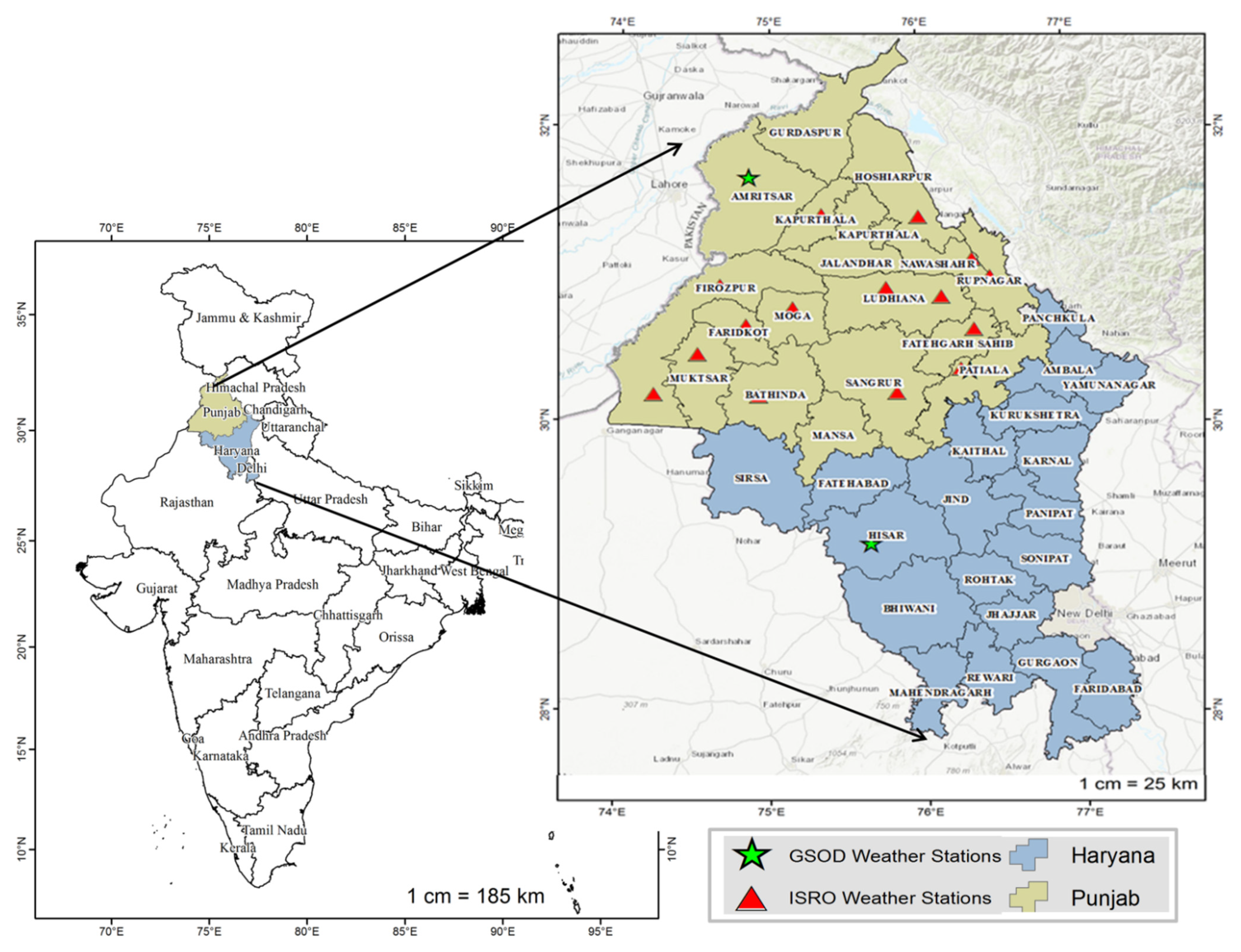
2.1. Study Area

The major wheat cultivating regions of Punjab and Haryana was chosen as the study area (Figure 1). Punjab and Haryana collectively contribute 30% of the total output with the highest productivity and roughly covers about 30% of the entire area under wheat, hence playing a significant role in the wheat economy of India. The study area has diverse climatic conditions, including arid, semi-arid and sub-humid climate types and topography comprising plains, undulating plains, dissected foot-hill zone and sub-mountain undulating region. The winter/rabi wheat growing period in the region extends from November to April, with maximum temperature ranging from 8 to 30 °C and minimum temperature varying from 3 to 20 °C. The winter season brings in disturbances, and considerable rainfall is observed. The sub-mountain regions of the domain receive about 100 mm rain during the winter season. Figure 2 shows the spatial map of rainfall and temperature averaged across the years 2001–2013 for the winter wheat growing season (November to April) to elucidate the spatial variability across the study region.

2.2. Weather Forecast Model—Model Specifications and Simulation Protocol

Weather Research and Forecasting (WRF) [24] model (version 3.4.1) is a regional climate model widely used to forecast/downscale micro-meteorological weather variables. In the study, WRF-ARW (Advanced Research WRF) core, a fully compressible non-hydrostatic (with hydrostatic option) system of equations, was used. WRF-ARW is a limited area model, which depends on the global models for initial and boundary conditions, and hence the forecast capability is reduced to the forecast lead time and the quality of the global models. Additionally, the artificial boundaries created from the use of different models having different model physics and dynamics had been proven to introduce errors in weather simulations [25]. Thus, Global version of WRF (GWRF), released in 2008 [26], was used in the study. GWRF is a functional system for nested non-hydrostatic global simulations and aims at coupling weather systems on global and regional scales with the same physics and dynamics options. Initial validation and global sensitivity studies [25] showed a better performance in capturing the global mean climatology.
The model was initialized with Global Forecast System (GFS) forecast data, downloaded at 0.5 degree resolution with 47 pressure levels. GWRF was set up with a global domain and two nests conforming to 1:5:5 ratios were implemented as two-way nesting. The model had 36 vertical levels with the top of the model atmosphere located at 10 hPa. The SST update was enabled in the parent domain to have a realistic pattern of the influences of the ocean in the atmospheric modelling for extended simulations. The physics options and model configurations are listed in Table 1. The critical land surface parameters, such as topography, landuse/landcover (LULC) and leaf area index (LAI) were altered in the study based on results from Kirthiga and Patel [23].
The forecast was performed for different time scales of 1, 2, 3 and 5 weeks before the harvest date. The average harvest date was selected to be 17 April 2009 for the study region through a combination of crop model simulations, MODIS LAI temporal products and state-wide reports. The details of the time period for each forecast are given in Table 1. Each simulation was initialized at 0300 Universal Time Coordinated (UTC) (to match with local time) and a spin-up time of two days was given. Forecasts of maximum temperature at 2 m; the minimum temperature at 2 m; solar radiation, and precipitation, relative humidity at 2 m; and wind speed at 10 metres were derived from the weather model.

2.3. Weather Forecast Model—Quality Assessment

Considering the main objective of the study (in-season wheat yield forecasting) and brevity of the manuscript, the accuracy of the generated weather forecasts is briefly discussed in this section. The forecasts from WRF model were validated with fifteen automatic weather stations (AWS) data, installed by Indian Space and Research Organization (ISRO) and three global summary of a day (GSOD) stations (NOAA 2010) within Punjab and Haryana (Figure 1). These stations were selected to ensure that they are spatially distributed, representing the variation in terrain and climatology across the study region. The bilinear interpolation method was used to select the representative/closest model grid cell, which was nearest to the observation station. Performance analysis for weather variables (minimum temperature at 2 m (°C), maximum temperature at 2 m (°C), relative humidity at 2 m (%), wind speed at 10 m (m/s), rainfall (mm) and solar radiation (MJ/m2)) were investigated for different lead-time scenarios.
Table 2 lists the root mean squared error (RMSE) values for the weather variables across the lead times. The simulated weather showed good agreement with the observed weather, yet the agreement decreased with increase in the lead-time. The continual growth and accumulation of error as a result of initial condition and model errors across the forecast times is a common challenge in medium/extended range weather forecasting [33,34]. However, the model produced least error for certain variables viz. minimum temperature, solar radiation and wind speed even with the longest lead time. Studies [35,36] have shown that the temperature is the most predictable parameter of the micrometeorological variables. In the present study, the minimum temperature had least error for all the lead times, when compared to the RMSE of maximum temperature, which showed steep increase with increase in lead time. In their study, de Perez et al. [36] recorded better performance of NWP models in forecasting cold waves over the tropics, while the predictability of heat extremes varied across space [37]. They also suggested that models that represent better land-surface interactions were likely to improve the predictability of the heat waves. Furthermore, the sharp increase in the error growth rate of maximum temperature across the higher lead times could be resultant from using GWRF for extended range forecasting (3 and 5 weeks). The operational global circulation models (GCMs) maintained by various governmental agencies are well formulated with sophisticated data assimilation systems and better representation of the land-sea interactions, when compared to GWRF. This could have led to the error growth getting amplified in the simulated variables. However, the other variables record lesser RMSE, owing to the simulation time of the year (peak summer in India—pre-monsoonal conditions), where high variability is present largely in the maximum temperature, when compared to the other micrometeorological variables [35].
The 1-, 2- and 3-weeks lead-time forecasts performed well for most of the variables (maximum temperature, minimum temperature and solar radiation). The 5-weeks forecast seemed to be slightly unsteady, considering the magnitude of errors and the increased uncertainty ranges (not shown here) for most of the variables. The inherent problems with using GWRF, when compared to the operational GCMs can be attributed as the major reason for the amplification of the errors in the longest forecast lead time (5 weeks). Since we did not have access to the extended range forecasts (3 and 5 weeks) from operational NWPs and we sought to quantify the utility of GWRF, the model was chosen for the study. The weather forecasts from GWRF were also compared with the National Center for Environmental Prediction (NCEP) Climate Forecast System Reanalysis (CFSR) (referred as NCEP hereafter in the article) data to quantify the spatial quality of the generated forecasts against the widely used NCEP data (in agricultural and hydrological impact studies). The NCEP mostly overestimated minimum temperatures, solar radiation, precipitation and wind speed, while it underestimated maximum temperatures and relative humidity. The biases were reduced with GWRF simulations with an average improvement factor of 30% over the NCEP data for the given season across all the observation stations.

2.4. Crop Simulation Model—Description

The Decision Support System for Agrotechnology Transfer (DSSAT) version 4.7 is a software application program that includes crop simulation models for over 28 crops [38]. The Crop Environment REsource Synthesis (CERES)-Wheat model [39] used in the study simulates growth, development and yield as a function of the soil-plant-atmosphere (SPAC) dynamics. The model has been popularly applied in a variety of applications, ranging from on-farm precision farming to regional impact assessment studies [40,41]. The driving variables are weather, soil, management parameters and cultivar-specific genetic coefficients, while the state parameters are LAI, biomass, yield. The model simulates the crop growth at a daily time step.
The methods used in the present study to represent critical processes within the model were exponential with LAI method for light interception accounting, radiation use efficiency (RUE) method for biomass production, FAO Penman-based evapotranspiration estimation, Soil Conservation Service (SCS) method for representing infiltration processes and Canopy Photosynthesis Response Curve method for photosynthesis calculation.

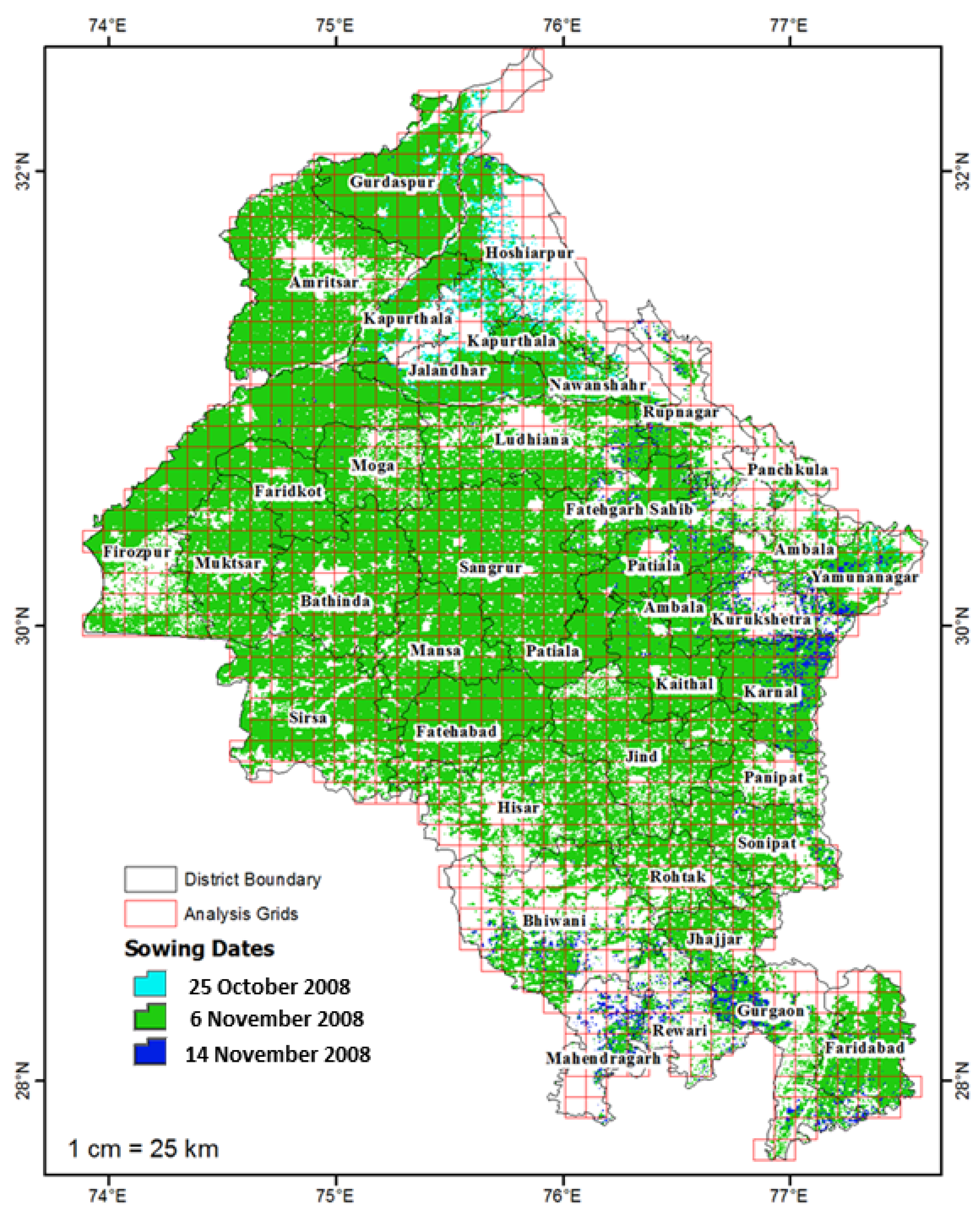
2.5. Gridded Implementation of the Crop Model—Input Data Preparation

The minimum data required for the crop model includes planting details, weather data, soil data, irrigation data, fertilizer data and plant species-specific genetic coefficients. The agricultural zones of Punjab and Haryana do not experience much of the limitation, as it is one of the best-managed regions in the country. With most of the districts having an irrigation extent greater than 90%, the average water used during wheat production ranges between 1900–3400 m3 per hectare [42] and the fertilizer consumption across the region is widely estimated to be greater than 200 kg per hectare [43]. Thus, the cropping area, sowing dates, weather and soil properties data were considered to be spatially varying, while the other inputs (crop cultivar, water and nutrient management) were considered spatially invariable throughout the study region. Gridded implementation was done with grid cells of 10 km × 10 km size (Figure 3), aligned to match with the outputs from the weather model. A total of 1040 grids covered the study region, and the center of each grid cell is the point-site used for DSSAT CERES-Wheat simulations. The methodology helped in enabling spatial mode for the DSSAT model.
Crop cultural and management practices followed in the simulation and are listed in Table 3. The assumption of one single cultivar throughout the regions of Punjab and Haryana might introduce some uncertainty in the methodology. However, PBW-343 was a mega-cultivar during the simulation period and occupied major area in north-western plains of India [44]. Additionally, the study focused on inter-comparison between various scenarios generated by altering the weather input, and thus the uncertainty in the inherent assumption (on the cultivar type) is common across the scenarios. The preliminary selection of the additional details on planting, irrigation and fertilizer applications were based on earlier studies on winter wheat in Punjab and Haryana [45,46].
The land use/land cover (LULC) data were acquired from the National Remote Sensing Centre (NRSC) for the time between 2008–2009, prepared at a scale of 1:250,000. The eight-day surface reflectance of MODIS was used to derive the enhanced vegetation index (EVI) at 500 m resolution for the whole crop period from September 2008 to May 2009. An algorithm similar to Vyas et al. [47] was used to identify wheat pixels from the temporal profile of EVI. The output was validated against the reported district-wise wheat area and an overall accuracy of 88% was obtained. The temporal profile (8-day composite) of EVI for the selected wheat pixels was smoothened using Savitzky-Golay filter to remove the noise in the data. The slope of the temporal profile was used to identify the inflection point and derive the sowing date [47]. Three sowing dates resulted, viz. 25 October 2008, 6 November 2008 and 14 November 2008, with the majority of pixels belonging to 6 November 2008 category. The dates matched very well with the national crop calendar and earlier studies [18]. Figure 3 exhibits the areal extent of wheat and the spatial spread of the sowing dates. The sowing date that had a maximum frequency within the 10 km grid cell was selected as the sowing date for the 10 × 10 km grid.
Soil properties survey data were obtained from soil resource database of India published by National Bureau of Soil Survey (NBSS) at 1:1 million scale. A total of 240 unique soil classes were derived from the data. DSSAT requires soil surface data, such as soil type and texture, surface slope, albedo, drainage rate and runoff curve number, which was derived from NBSS soil survey map. The model also requires soil horizon data where the field capacity equivalent, permanent wilting point equivalent, field saturation, saturated hydraulic conductivity, root growth factor and physical and chemical properties need to be specified. All the above-mentioned parameters were assumed based on soil taxonomy classes from the soil map. The major soil type from the NBSS survey map within each grid cell was selected for simulation at 10 km resolution.
National Center for Environmental Prediction (NCEP) Climate Forecast System Reanalysis (CFSR) was completed over a 36-year period (1979–2014) [48]. The NCEP was executed as a high-resolution atmosphere-ocean-land-surface-sea-ice coupled global model, intended to provide the best estimate of the state of the atmosphere. All the available conventional and satellite observations were assimilated into the NCEP-CFSR model. The data were downloaded in daily time steps at a spatial resolution of 25 km. NCEP had been suggested as a valid option for regional analysis when weather stations are not evenly distributed [49,50]. Bi-linear interpolation method was used to downscale the 25 km resolution NCEP data to match with the WRF resolution (10 km). Bi-linear interpolation was considered to be sufficiently adequate for interpolating smoothly varying variables [51].

2.6. Crop Simulation Model—Calibration and Sensitivity Analysis

A sensitivity study (manual method) for the CERES-Wheat model was done to understand the most sensitive parameters. The cultivar-specific parameters, such as genetic, ecotype and phenology parameters, were considered for calibration based on results of sensitivity analysis. MODIS leaf area index (LAI), at a spatial resolution of 1 km and temporal resolution of 8-day, was also used for the calibration along with district-level yields. In general, the temporal evolution of biomass can be closely correlated with LAI, and thus calibration with satellite-derived LAI was considered to be more realistic [52]. The crop season of 2007–2008 was used for calibration, while 2008–2009 was used for validation of the parameter values. Both the selected crop years (2007–2008 with yield of 4507 kg/ha and 2008–2009 with yield of 4462 kg/ha) were normal years with much less deviation from average wheat yield of 4410 kg/ha (calculated from 2000–2011 wheat crop yields in the states). The results of sensitivity analysis, calibration and validation are discussed in the results section.

2.7. Simulation Experiments and Validation

A total of five forecast scenarios were generated to forecast crop yield at different lead times by varying only the weather input. The details of the scenarios are given in Table 4.
The simulated yields at 10 km resolution were aggregated (area-weighted averaging) at the district level and validated with district-level actual yields obtained from the crop cutting experiments by the state agricultural department. The NCEP weather data-based crop yield simulation for the whole growing season of 2008–2009 was used as reference simulation (abbreviated as F1). The other simulations were compared against the reference simulation and relative improvements were also addressed.
To validate regional crop simulations at a higher spatial resolution than just with district-level aggregations, MODIS LAI was used. The maximum values (across the season) of the simulated LAI were validated against the maximum values of the MODIS LAI for every grid. The maximum leaf area of wheat was considered, since it had been widely correlated to yield. Studies [53,54] have shown that the maximum leaf area is attained 10–20 days before flowering/heading to 10 days after flowering/heading in wheat, which is the critical period impacting the magnitude of yield. Since the forecast scenarios, F2 and F3, were close to harvest date, the spatial validation procedure was restricted to F1, F4 and F5, where the variations in leaf area index were substantial. The suggested procedure was demonstrated to be reasonable for validating crop simulation performance on a regional scale, given that other sources of finer/sub-regional scale yield/state variable (biomass, LAI) estimates were not available [55].
The statistical measures, such as root mean square error (RMSE), mean bias (MB), mean absolute percent error (MAPE), relative deviation (RD), R-squared (R2) and agreement index were used to evaluate the performance of the crop model simulations. Another statistic, improvement factor for evaluating the percent improvement of a simulation over another simulation, was also used [56].

3. Results

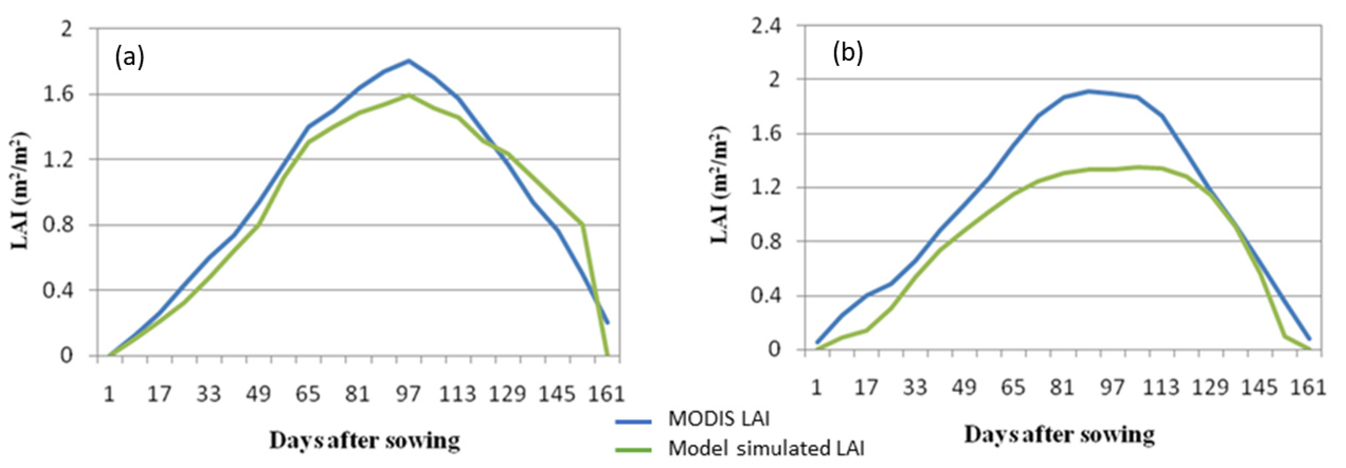
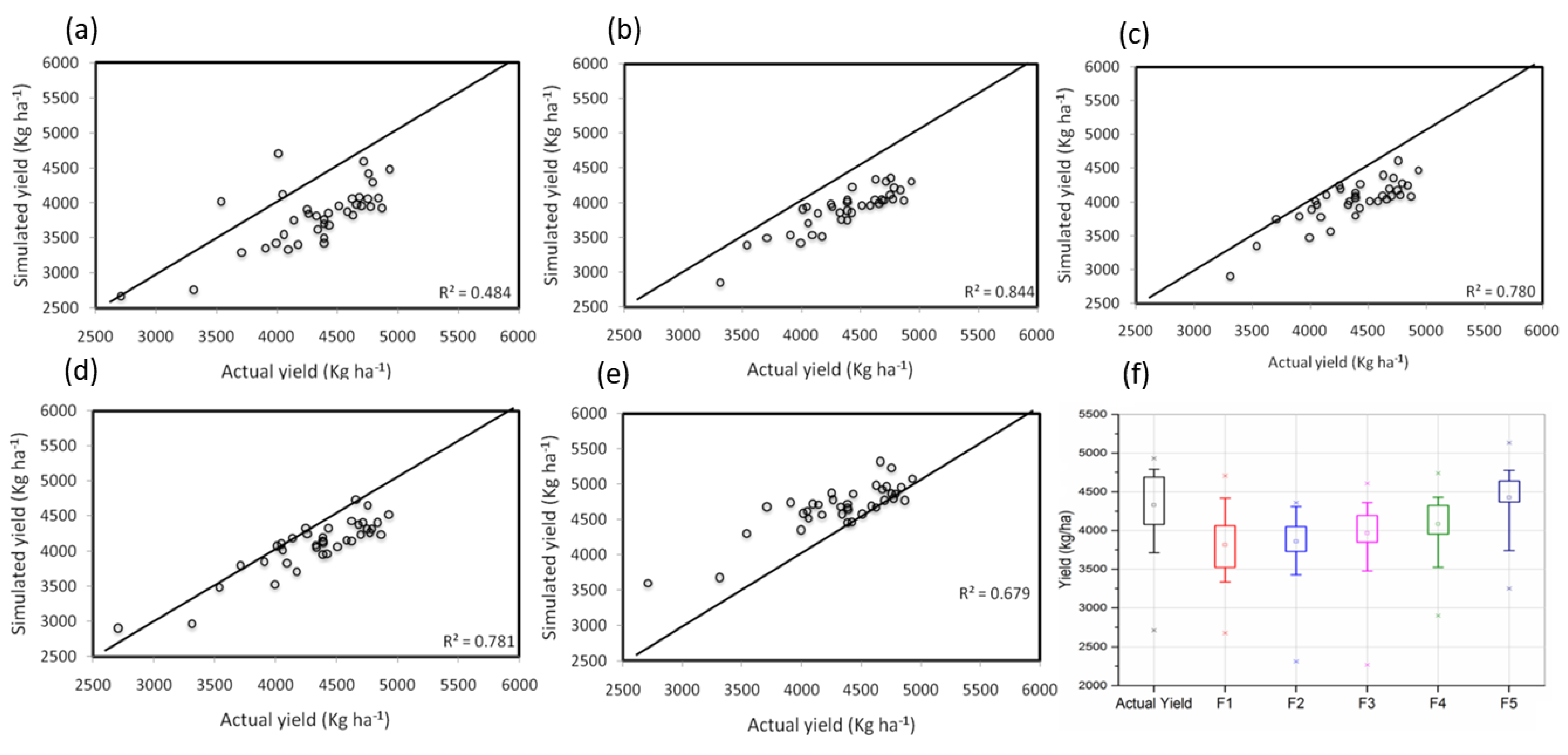
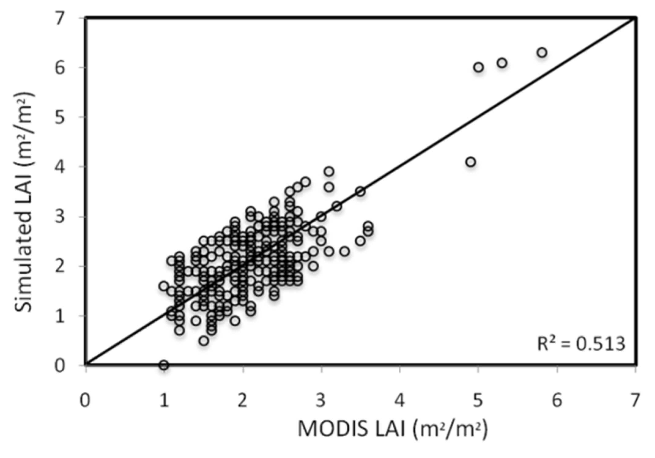
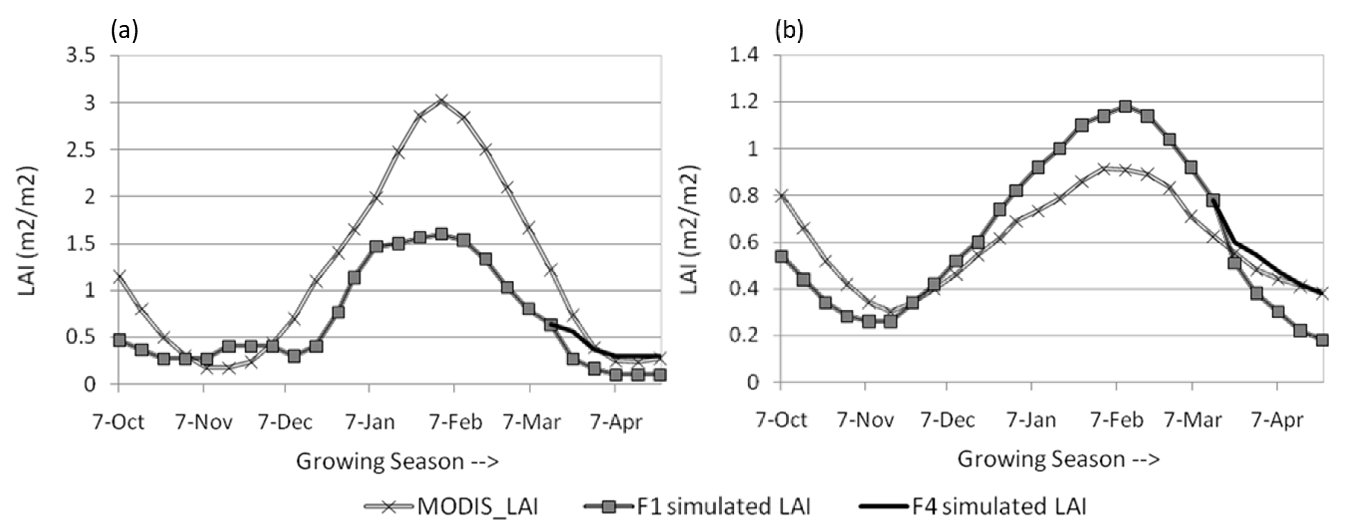
3.1. Calibration and Validation of Crop Model

The results of sensitivity analysis showed that the model was highly sensitive to photo-synthetically active radiation (PAR) conversion to dry matter ratio before the last leaf stage (PARUV) parameter. A +/− 10% change from the optimal value of PARUV has a +/− 5–7% impact on the simulated yield values. Vernalization sensitivity coefficient (P1 V) had a considerable impact on the model simulated yields, a +/− 25% change caused a +/− 6–10% change in the yield values. Potential kernel growth rate (G2) parameter underestimated (over-estimated) the yield when reduced (increased) from optimal values. A +/− 10% change in G2 values impacted +/− 2–3% of simulated yield. The Kernel number per unit stem to the spike weight at anthesis (G1) also had an impact on the model’s simulations and an increase/decrease in the value-simulated low yields, while optimal value maximized the simulated yield. Model simulation was significantly impacted by temperature response during grain filling, especially by the optimal temperatures for increase in grain weight (T (opt1), T (opt2)) parameter values. Crop model was also found to be significantly sensitive to other parameters, such as P1, P2, P3 and PHINT.
Calibration was performed with the identified sensitive parameters at a spatial scale. At the end of calibration, the model simulating LAI and crop yield was in close agreement with the satellite observed values. The relative deviation for LAI and yield were −8.9% and −4%, respectively. The simulated LAI recorded an RMSE of 0.15 m2/m2 and an r-squared value of 0.91 (Figure 4a).
Figure 4b shows the validation of the model’s performance with calibrated parameters for the crop season of 2008–2009. Appreciable agreement of 85% was obtained with an RMSE of 0.4 m2/m2 and r-squared of 0.78. The LAI and yield simulations recorded a relative deviation of −9.5% and −6.3%, respectively. There is a wide disagreement between the MODIS LAI and the model simulated LAI during the peak growing season and during both calibration and validation periods. Overfitting the model simulated LAI values to match MODIS LAI caused a higher deviation from observed yields. One probable reason could be the inherent overestimation concerns with MODIS LAI algorithm for vegetation, as reported by Yang et al. [57]. Additionally, MODIS LAI is not particularly intended for retrieval of deterministic LAI values and the errors due to pixel geolocation mismatch might have introduced deviations [57]. Table 5 tabulates the adjusted values of the sensitive parameters after calibration and validation of the crop model.

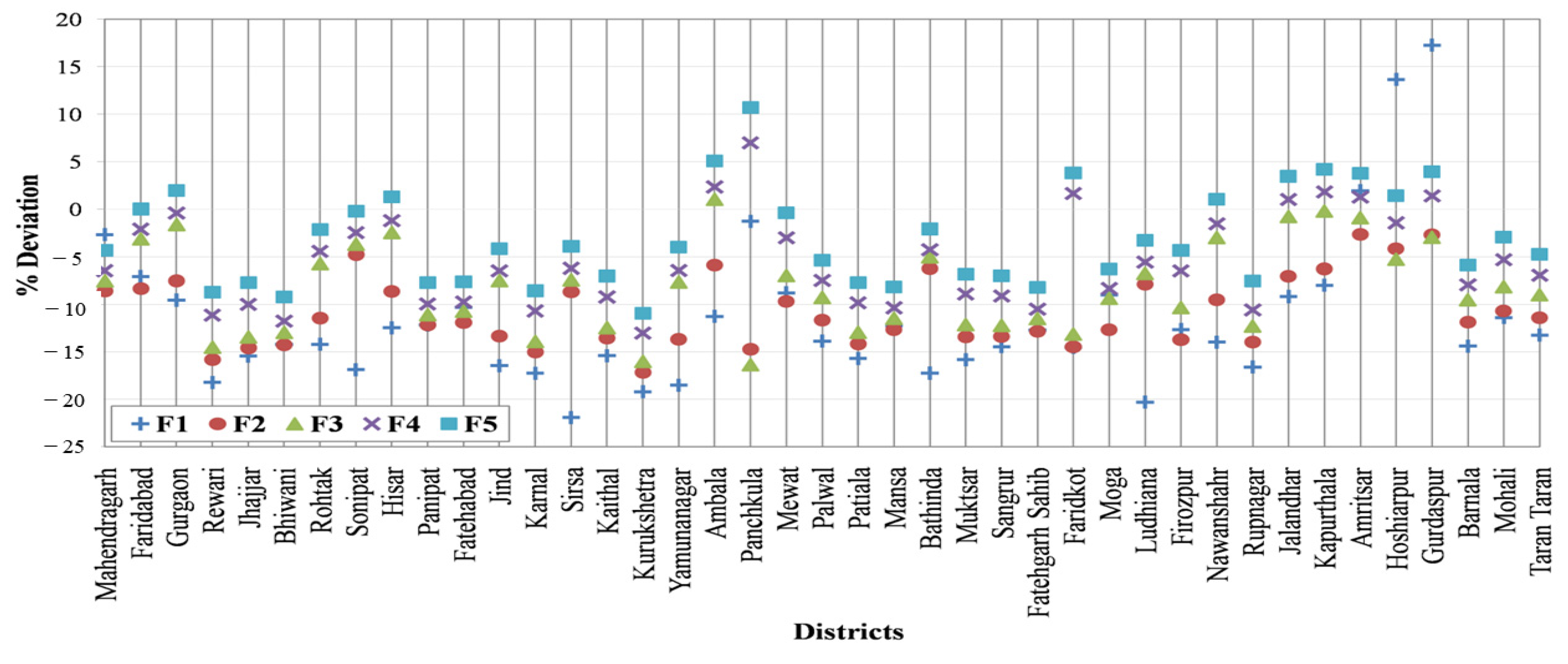
3.2. District-Wise Aggregated Yields

The district-level aggregated yields showed good agreement with the actual yields. The RMSE, MAPE, RD and agreement index for different forecast scenarios are tabulated in Table 6. Maximum RMSE of 622.52 kg/ha was recorded in the F1 forecast scenario (NCEP-CFSR weather data), capturing only 66% of the variability in the yield. The F4 (3 weeks prior to harvest forecasts) simulated yields were in close agreement with the actual yields giving the least RMSE of 327.75 kg/ha and 86% agreement with the reported yields. The F5 (5 weeks prior to harvest forecasts) scenario recorded RMSE of 415 kg/ha with 41% agreement index. The F5 case highly over-predicted the yield with a relative deviation of 8.91%, while the other forecasts recorded an under-prediction in yield values across the districts (Figure 5). Figure 6 shows the spatial distribution of predicted yield. The districts of Panchkula and Amristar recorded the lowest deviations with F1 and F2 simulations. The districts Kapurthala, Jalandhar and Amritsar gave good results with the F3 scenario. Many districts performed well in the F4 scenario with an average RD of –3.1, yet a few districts, such as Kurukshetra, Bhiwani, Rewari and Karnal, showed an average relative deviation of –10%, and Ambala recorded 4% relative deviation. In the F5 scenario, major underestimation (RD of –17%) was observed in Fatehgarh Sahib, Faridabad and Moga districts, while Ambala, Hoshiarpur, Panchkula, Nawanshahr (now known as Shaheed Bhagat Singh Nagar district), and Kapurthala showed substantial overestimation (RD of 17%) of yield in the F5 scenario. Figure 7a–e show the correlation plots for yield simulations across the forecast scenarios with the r-squared values. Figure 7f exhibits the box plots of the simulated yield values against the actual yield values.

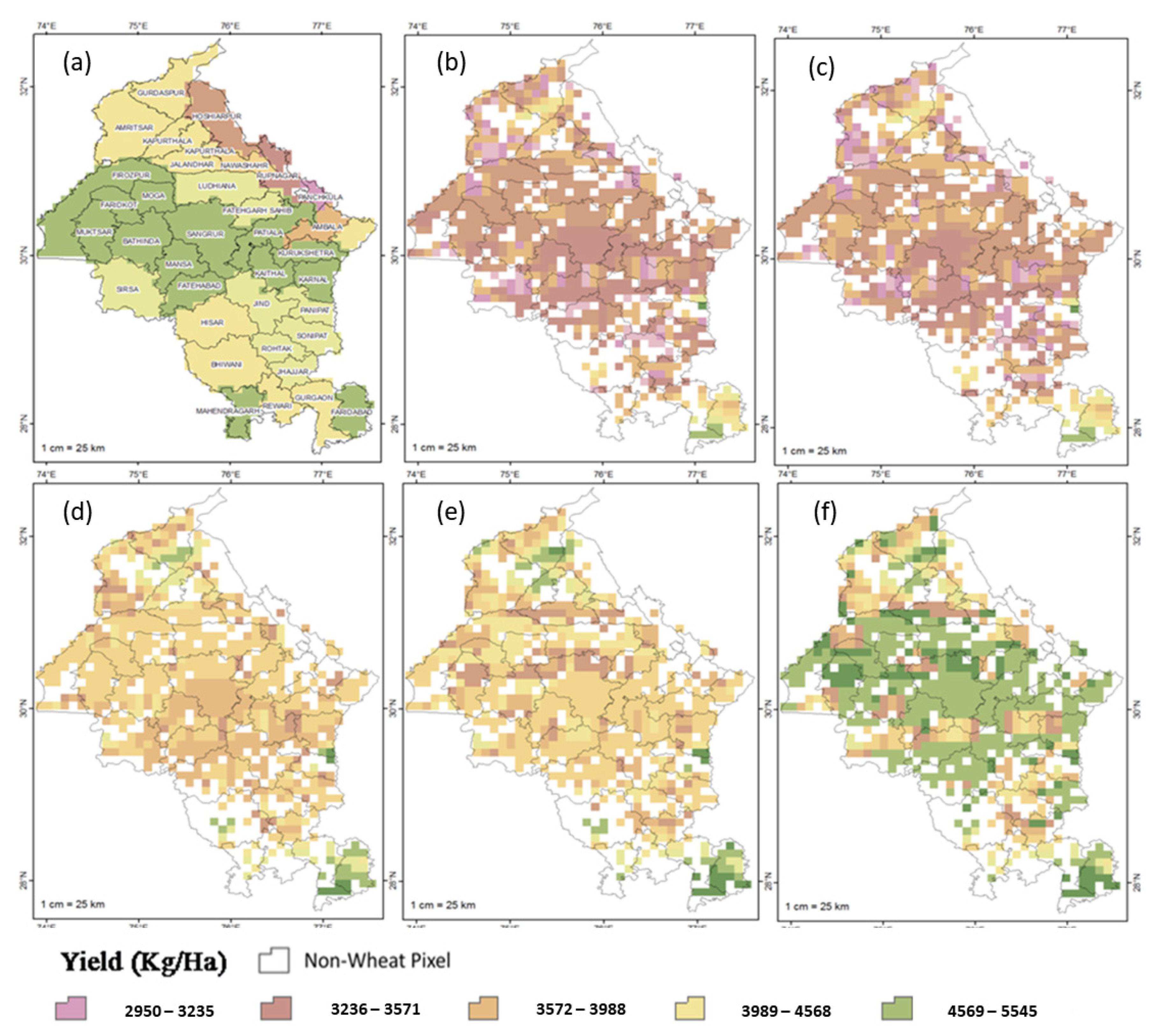
3.3. Spatial Variability Yield Simulations

The LAI maximum values across the season obtained from MODIS and model simulation with the F1 scenario is shown in Figure 8. In general, the LAI maximum values were attained 10–20 days before flowering and the model simulated LAI maximum reflected NCEP weather data for most of the forecast cases. Thus, F4 and F5 showed similar behavior as that of F1 with no significant deviation. The comparison served to understand the spatial performance of the simulated LAI values (as proxy for yield). An average RD of –0.17% and mean bias of −0.3 m2/m2 was observed between F1-simulated LAI and MODIS LAI. The low and high bias values were −2.5 m2/m2 and +1.85 m2/m2, respectively. The LAI values in districts Sangrur, Ludhiana, Kaithal, Mansa, Patiala, Kapurthala, Jind and Karnal were widely underestimated (−1 to −0.5% deviation), while in districts Rupnagar, Firozpur, Muktsar, Sirsa and Hoshiarpur, the values showed over-estimation (1 to 2% deviation). This is evident from the 1:1 correlation plot (Figure 9) with a moderate value of coefficient of determination (R2 = 0.51).
The spatial yields generated for Punjab and Haryana states are shown in Figure 6. As mentioned earlier, the F1 scenario was assumed to be the best attainable spatial yield output at the present data-scarce condition. The relative deviation from the reference yield was calculated for the other scenarios. F2 showed a negligible deviation of 2–4% across all the districts. The F3 scenario showed an RD of 15–19% for pixels in districts of Gurdaspur, Hoshiarpur, Sirsa and Rothak. It also recorded an RD of −2.2% for few parts of Rupnagar. F4 scenario showed a significant deviation of 17–28% for parts of Sangrur, Mansa, Sirsa, Hisar, Muktsar, Karnal and Faridabad districts. Some pixels in Panchkula, Ambala and Rupnagar recorded RD of −4.5%. An RD of 35–42% was observed in the F5 case for parts of Ambala, Panchkula, Rupnagar, Karputhala, Kurukshetra, Faridabad and Patiala. Parts of Bathinda, Rothak and Fatehgarh Shaib recorded a −2% relative deviation from the F1 scenario.

4. Discussion

The forecast scenarios F1, F2, F3 and F4 have performed well for low-yielding and medium-yielding districts, while they have widely underestimated yield in the high-yielding districts (Figure 6). The WRF forecasts were coupled with the NCEP merely after the flowering stage in the present study, where the critical stages (peak vegetative stages and flowering stages) were represented by weather data from NCEP-CFSR data. As discussed earlier, the NCEP data had intrinsic biases, and the uncertainties introduced from the interpolation method used caused non-realistic conditions, consequently, leading to the underestimation of yield in the forecast scenarios. Table 7 shows the optimal values of weather variables required at different growing stages. The overestimation of minimum temperatures, underestimation of relative humidity, overestimation of wind speed, unrealistic rainfall values in the NCEP data have hindered the crop model from realizing the actual yield. Figure 8 captures the spatial ambiguity, where the F1 scenario had greatly underestimated the LAI values during the peak growing stage for the high-yielding districts in central Punjab (Sangrur, Ludhiana and Patiala) and Haryana (Kurukshetra, Kaithal, Jind and Karnal).
The underestimation (Figure 6 and Figure 7) decreased with the increase in lead time until F4 (3 weeks prior to harvest forecast), which was due to the improvement of WRF forecasts over the NCEP data for critical weather variables. The F2 showed much less deviation from F1, since the modification of the weather was done only towards the end of growing season, where the crop is fully matured and ready for harvest. F3 recorded a significant impact, since it had improved weather inputs during the final stages of maturity in early-sown crops and the intermediate stages of maturity in late-sown crops. Thus, the high-yielding (Figure 6a), late-sown crops (Figure 3) in the districts of Kurukshetra, Karnal, Kapurthala and Jalandhar were well simulated with F3 (Figure 6d and Figure 7c). F4 was the best performing case-improving yield simulations for most of the districts (Figure 6e). The F4 forecast replaced the NCEP weather data from early maturity for early-sown crops and the intermediate to final stages of grain filling in the late-sown crops. LAI plots for the low-yielding district (Rupnagar) and high-yielding district (Sangrur) are shown in Figure 10. Although the post-maturity LAI values have no major impact on yield simulations, the improvement in the LAI profile demonstrates the reduction in deviation by F4 scenario. Despite the fact that the weather for 3 weeks prior to harvesting forecasts had biases, they were well within the optimal range (Table 7), representing close to the real-time scenario and, subsequently, simulating better yields. In addition, the F4 simulation had performed well for some high-yielding districts and all medium- and low-yielding districts. Some of the high-yielding districts, particularly the early-sown regions were not well simulated, owing to the biases in NCEP data and due to the issues with calibration, as discussed earlier.
The F5 forecast scenario behaved slightly differently from the other cases. The scenario had improved yield estimations for the districts in plains, while the districts that lie in sub-mountainous regions performed to a lower level. There was significant over-prediction for the yields in those districts due to the substantial bias in the weather simulations for the 5 weeks prior to the harvest weather forecast [14]. These regions exhibited an under-prediction of minimum temperatures and solar radiation, with over-prediction of relative humidity in the 5 weeks prior to harvest forecasts. Thus, the scenario had represented unrealistically optimal conditions for the crop growth, consequently, leading to the overestimation of yields. The F5 case had performed well for some districts in the plains, where the bias in the 5 weeks prior to harvest weather forecast was comparatively less. However, the error was reduced when the results were aggregated at district level. Since the implementation was at a spatial scale and in combination with the NCEP data, the impact was not linear, as in case of a similar study by Togliatti et al. [14]. The 3 weeks ahead of harvest forecasts performed well in capturing the spatial yield variability [58].

5. Conclusions

The study is a unique effort to test the applicability of using an improved version of NWP-generated forecasts for extended range regional level end-of-season yield predictions. The major objectives of the present study were (1) obtaining weather forecasts at various lead times from regional NWP, (2) setting up of gridded crop simulation model after calibration and validation exercise, (3) coupling of weather and crop models to assess the predictability of within-season wheat yield at sub-regional scales.
The forecast length of the weather forecasts caused significant impact on the accuracy of the simulated yield [59]. However, since the implementation was on spatial scale and in combination with the NCEP data, the impact was not linear as in case of a similar study by Togliatti et al. [14]. The 3-weeks ahead of harvest forecasts performed well in capturing the spatial yield variability. Two major observations were recorded, the critical crop growth stages were highly sensitive to the errors in weather forecasts and district-level aggregations were helpful in averaging out the spikes created by uncertain weather forecasts. It is also evident from the results that the complexity of crop-weather interactions decreases towards the end of the growing season, and thus a reasonable representation of weather with known uncertainty ranges are essentially sufficient [58].
The results highlight that there is a definite requirement to reduce the input and model-based errors in mesoscale weather modelling. Data assimilation techniques can help in improving the initial and lateral boundary conditions [60]. Ensemble methods can increase the uncertainty ranges being represented within the weather model [61]. Bias correction of the near-surface simulated weather would also help in improving spatial yield predictions [10,58,62]. Recommendations from the Agricultural Model Intercomparison and Improvement Project (AgMIP) [63] state that the gridded model output needs to be quantified for uncertainty by comparison with observed site information, and the bias correction factors require global development. They strongly believe that the bias corrected gridded output can provide vital feedbacks to develop hybrid response systems across the globe. Spatial-wide calibration and data assimilation strategies need to be strengthened for spatial implementation of crop growth models [64].
The current work is highly relevant to develop quick response systems during region-wide crop production failures/surplus and to handle market uncertainties in changing climatic regimes. This study is a unique effort in coupling the climate and crop model for generating real-time extended in-season yield predictions at finer regional scales. The results of the preliminary study were satisfactory and offer a vast scope for practical application. Future research will be focused on intensive testing of the methodology for other seasons, years and crops across the country.

Author Contributions

S.M.K.—Conception and design of the study; data download and processing, analysis and interpretation of data; drafting of the manuscript and approval of the version of the manuscript to be published and corresponding author. N.R.P.—Conception of the study, providing resources, revising the manuscript critically for important intellectual content and approval of the version of the manuscript to be published. All authors have read and agreed to the published version of the manuscript.

Funding

This research received no external funding.

Institutional Review Board Statement

Not Applicable.

Informed Consent Statement

Not Applicable.

Data Availability Statement

Datasets are publicly available from MOSDAC-SAC (https://mosdac.gov.in/catalog/satellite.php, accessed on 1 January 2020), Bhuvan-NRSC (https://bhuvan-app3.nrsc.gov.in/data/download/index.php, accessed on 1 January 2020), LP-DAAC-NASA (https://lpdaac.usgs.gov/data/, accessed on 1 January 2020) and NCEP (https://catalog.data.gov/dataset/noaa-ncep-global-forecast-system-gfs-atmospheric-model, accessed on 1 January 2020).

Acknowledgments

Authors express sincere thanks to the director of the IIRS for the motivation, encouragement and facilities to perform research on weather modeling. Special thanks to R. Jaganathan, professor of agronomy in the Agro-Climatic Research Centre, Tamilnadu Agricultural University, India, for technical guidance on the WRF model. Authors also wish to thank various individuals and organizations, such as the director of the Space Application Centre (India); the director of the National Remote Sensing Centre (India), and USGS-EROS Center (USA), for providing easy access to in situ weather data, land cover and biophysical databases.

Conflicts of Interest

The authors declare no conflict of interest.

References

  1. Fischer, T. Wheat yield losses in India due to ozone and aerosol pollution and their alleviation: A critical review. Outlook Agric. 2019, 48, 181–189. [Google Scholar] [CrossRef]
  2. MoA&FW. Ministry of Agriculture and Farmers Welfare, Government of India. 2018. Available online: https://eands.dacnet.nic.in/Advance_Estimate/4th_Adv_Estimates2017-18_Eng.pdf (accessed on 25 June 2020).
  3. Ortiz-Monasterio, R.J.I.; Dhillon, S.S.; Fischer, R.A. Date of sowing effects on grain yield and yield components of irrigated spring wheat cultivars and relationships with radiation and temperature in Ludhiana, India. Field Crop. Res. 1994, 37, 169–184. [Google Scholar] [CrossRef]
  4. Ju, W.; Gao, P.; Zhou, Y.; Chen, J.M.; Chen, S.; Li, X. Prediction of summer grain crop yield with a process-based ecosystem model and remote sensing data for the northern area of the Jiangsu Province, China. Int. J. Remote Sens. 2010, 31, 1573–1587. [Google Scholar] [CrossRef]
  5. Siderius, C.; Hellegers, P.J.G.J.; Mishra, A.; van Ierland, E.C.; Kabat, P. Sensitivity of the agroecosystem in the Ganges basin to inter-annual rainfall variability and associated changes in land use. Int. J. Clim. 2014, 34, 3066–3077. [Google Scholar] [CrossRef] [Green Version]
  6. Pramod, V.; Rao, B.B.; Ramakrishna, S.; Singh, M.M.; Patel, N.; Sandeep, V.; Rao, V.; Chowdary, P.S.; Kumar, P.V. Impact of projected climate on wheat yield in India and its adaptation strategies. J. Agrometeorol. 2017, 19, 207–216. [Google Scholar] [CrossRef]
  7. Basso, B.; Liu, L. Seasonal crop yield forecast: Methods, applications, and accuracies. Adv. Agron. 2018, 154, 201–255. [Google Scholar] [CrossRef]
  8. De Wit, A.; Baruth, B.; Boogaard, H.; van Diepen, K.; van Kraalingen, D.; Micale, F.; te Roller, J.; Supit, I.; van den Wijngaart, R. Using ERA-INTERIM for regional crop yield forecasting in Europe. Clim. Res. 2010, 44, 41–53. [Google Scholar] [CrossRef]
  9. Malherbe, J.; Landman, W.; Olivier, C.; Sakuma, H.; Luo, J.-J. Seasonal forecasts of the SINTEX-F coupled model applied to maize yield and streamflow estimates over north-eastern South Africa. Meteorol. Appl. 2014, 21, 733–742. [Google Scholar] [CrossRef]
  10. Peng, B.; Guan, K.; Pan, M.; Li, Y. Benefits of Seasonal Climate Prediction and Satellite Data for Forecasting U.S. Maize Yield. Geophys. Res. Lett. 2018, 45, 9662–9671. [Google Scholar] [CrossRef]
  11. Jha, P.K.; Athanasiadis, P.; Gualdi, S.; Trabucco, A.; Mereu, V.; Shelia, V.; Hoogenboom, G. Using daily data from seasonal forecasts in dynamic crop models for yield prediction: A case study for rice in Nepal’s Terai. Agric. For. Meteorol. 2019, 265, 349–358. [Google Scholar] [CrossRef]
  12. Sillmann, J.; Thorarinsdottir, T.; Keenlyside, N.; Schaller, N.; Alexander, L.V.; Hegerl, G.; Seneviratne, S.I.; Vautard, R.; Zhang, X.; Zwiers, F.W. Understanding, modeling and predicting weather and climate extremes: Challenges and opportunities. Weather Clim. Extremes 2017, 18, 65–74. [Google Scholar] [CrossRef]
  13. Hanley, D.E.; Jagtap, S.; LaRow, T.E.; Jones, J.W.; Cocke, S.; Zierden, D.; O’brien, J.J. The Linkage of Regional Climate Models to Crop Models. American Meteorological Society Annual Meeting. 2002. Available online: https://ams.confex.com/ams/pdfpapers/25936.pdf (accessed on 1 October 2020).
  14. Togliatti, K.; Archontoulis, S.V.; Dietzel, R.; Puntel, L.; VanLoocke, A. How does inclusion of weather forecasting impact in-season crop model predictions? Field Crop. Res. 2017, 214, 261–272. [Google Scholar] [CrossRef] [Green Version]
  15. Richardson, D. Medium- and Extended-Range Ensemble Weather Forecasting; Palgrave Macmillan: Cham, Switzerland, 2018; pp. 109–121. [Google Scholar] [CrossRef] [Green Version]
  16. Lobell, D.B.; Sibley, A.; Ortiz-Monasterio, J.I. Extreme heat effects on wheat senescence in India. Nat. Clim. Chang. 2012, 2, 186. [Google Scholar] [CrossRef]
  17. Liu, B.; Liu, L.; Tian, L.; Cao, W.; Zhu, Y.; Asseng, S. Post-heading heat stress and yield impact in winter wheat of China. Glob. Chang. Biol. 2013, 20, 372–381. [Google Scholar] [CrossRef]
  18. Kaur, P.; Singh, H.; Rao, V.U.M.; Hundal, S.S.; Sandhu, S.S.; Nayyar, S.; Rao, B.B.; Kaur, A. Agrometeorology of Wheat in Punjab State of India; Technical report; Punjab Agricultural University: Ludhiana, India, 2015. [Google Scholar] [CrossRef]
  19. Sonkar, G.; Mall, R.; Banerjee, T.; Singh, N.; Kumar, T.L.; Chand, R. Vulnerability of Indian wheat against rising temperature and aerosols. Environ. Pollut. 2019, 254, 112946. [Google Scholar] [CrossRef]
  20. Njiti, V.N.; Myers, O.M., Jr.; Schroeder, D.; Lightfoot, D.A. Roundup Ready Soybean: Glyphosate Effects on Fusarium solani Root Colonization and Sudden Death Syndrome. Agron. J. 2003, 95, 114–125. [Google Scholar] [CrossRef]
  21. Marletto, V.; Ventura, F.; Fontana, G.; Tomei, F. Wheat growth simulation and yield prediction with seasonal forecasts and a numerical model. Agric. For. Meteorol. 2007, 147, 71–79. [Google Scholar] [CrossRef]
  22. Zhuo, W.; Fang, S.; Gao, X.; Wang, L.; Wu, D.; Fu, S.; Wu, Q.; Huang, J. Crop yield prediction using MODIS LAI, TIGGE weather forecasts and WOFOST model: A case study for winter wheat in Hebei, China during 2009–2013. Int. J. Appl. Earth Obs. Geoinf. ITC J. 2021, 106, 102668. [Google Scholar] [CrossRef]
  23. Kirthiga, S.M.; Indian Institute of Remote Sensing (IIRS); Patel, N.R. Impact of updating land surface data on micrometeorological weather simulations from the WRF model. Atmósfera 2018, 31, 165–183. [Google Scholar] [CrossRef] [Green Version]
  24. Skamarock, W.; Klemp, J.; Dudhia, J.; Gill, D.; Barker, D.; Duda, M.; Huang, X.; Wang, W.; Powers, J. A Description of the Advanced Research WRF Version 3. NCAR/TN-475 STR; NCAR Technical Note; Mesoscale and Microscale Meteorology Division, National Center of Atmospheric Research: Boulder, CO, USA, 2008; p. 113. [Google Scholar]
  25. Zhang, Y.; Hemperly, J.; Meskhidze, N.; Skamarock, W.C. The Global Weather Research and Forecasting (GWRF) Model: Model Evaluation, Sensitivity Study, and Future Year Simulation. Atmospheric Clim. Sci. 2012, 2, 231–253. [Google Scholar] [CrossRef] [Green Version]
  26. Richardson, M.I.; Toigo, A.D.; Newman, C.E. PlanetWRF: A general purpose, local to global numerical model for planetary atmospheric and climate dynamics. J. Geophys. Res. 2007, 112. [Google Scholar] [CrossRef]
  27. Kain, J.S. The Kain-Fritsch convective parameterization: An update. J. Appl. Meteorol. Climamatol. 2004, 43, 170–181. [Google Scholar] [CrossRef]
  28. Lin, Y.L.; Farley, R.D.; Orville, H.D. Bulk parameterization of the snow field in a cloud model. J. Clim. Appl. Meteorol. 1983, 22, 1065–1092. [Google Scholar] [CrossRef]
  29. Hong, S.-Y.; Noh, Y.; Dudhia, J. A New Vertical Diffusion Package with an Explicit Treatment of Entrainment Processes. Mon. Weather Rev. 2006, 134, 2318–2341. [Google Scholar] [CrossRef] [Green Version]
  30. Mlawer, E.J.; Taubman, S.J.; Brown, P.D.; Iacono, M.J.; Clough, S.A. Radiative transfer for inhomogeneous atmospheres: RRTM, a validated correlated-k model for the longwave. J. Geophys. Res. 1997, 102, 16663–16682. [Google Scholar] [CrossRef] [Green Version]
  31. Dudhia, J. Numerical study of convection observed during the winter monsoon experiment using a mesoscale two-dimensional model. J. Atmos. Sci. 1989, 46, 3077–3107. [Google Scholar] [CrossRef]
  32. Chen, F.; Dudhia, J. Coupling an advanced land-surface–hydrology model with the Penn State–NCAR MM5 modelling system. Part I. Model description and implementation. Mon. Weather Rev. 2001, 129, 569–585. [Google Scholar] [CrossRef]
  33. Lorenz, E.N. Effects of Analysis and Model Errors on Routine Weather Forecasts. In Proceedings of the ECMWF Seminars on Ten Years of Medium-Range Weather Forecasting, Reading, UK, 4–8 September 1989. [Google Scholar]
  34. Cooper, F.C.; Düben, P.D.; Denis, C.; Dawson, A.; Ashwin, P. The Relationship between Numerical Precision and Forecast Lead Time in the Lorenz’95 System. Mon. Weather Rev. 2020, 148, 849–855. [Google Scholar] [CrossRef]
  35. Haiden, T.; Bidlot, J.; Ferranti, L.; Bauer, P.; Dahoui, M.; Janousek, M.; Prates, F.; Vitart, F.; Richardson, D.S. Evaluation of ECMWF Forecasts, including 2014–2015 Upgrades. Technical Report 765, ECMWF. 2015. Available online: www.ecmwf.int/en/elibrary/miscellaneous/14691-evaluationecmwf-forecasts-including-2014-2015-upgrades (accessed on 1 January 2022).
  36. de Perez, E.C.; van Aalst, M.; Bischiniotis, K.; Mason, S.; Nissan, H.; Pappenberger, F.; Stephens, E.; Zsoter, E.; Hurk, B.V.D. Global predictability of temperature extremes. Environ. Res. Lett. 2018, 13, 054017. [Google Scholar] [CrossRef]
  37. Mandal, R.; Joseph, S.; Sahai, A.K.; Phani, R.; Dey, A.; Chattopadhyay, R.; Pattanaik, D.R. Real time extended range prediction of heat waves over India. Sci. Rep. 2019, 9, 908. [Google Scholar] [CrossRef] [Green Version]
  38. Hoogenboom, G.; Jones, J.W.; Porter, C.H.; Wilkens, P.W.; Boote, K.J.; Batchelor, W.D.; Hunt, L.A.; Tsuji, G.Y. Decision Support System for Agrotechnology Transfer (DSSAT) Version 4.5; University of Hawaii: Honolulu, HI, USA, 2012. [Google Scholar]
  39. Godwin, D.C.; Ritchie, J.T.; Singh, U.; Hunt, L. A User’s Guide to CERES-Wheat v2.1; International Fertilizer Development Centre: Muscle Shoals, AL, USA, 1989; Available online: https://nowlin.css.msu.edu/wheat_book/ (accessed on 1 January 2022).
  40. Buttar, G.S.; Jalota, S.K.; Mahey, R.K.; Aggarwal, N. Early Prediction of Wheat Yield in South-Western Punjab Sown by Different Planting Methods, Irrigation Schedule and Water Quality using the CERES Model. J. Agric. Phys. 2006, 1, 46–50. [Google Scholar]
  41. Singh, K.K.; Baxla, A.K.; Mall, R.K.; Singh, P.K.; Balasubramanyam, R.; Garg, S. Wheat yield prediction using CERES-Wheat model for decision support in agro-advisory. Vayu Mandal 2010, 5, 97–109. [Google Scholar]
  42. Sarkar, A.; Sen, S.; Kumar, A. Rice–wheat cropping cycle in Punjab: A comparative analysis of sustainability status in different irrigation systems. Environ. Dev. Sustain. 2008, 11, 751–763. [Google Scholar] [CrossRef]
  43. Majumdar, K.; Jat, M.L.; Pampolino, M.; Dutta, S.; Kumar, A. Nutrient management in wheat: Current scenario, improved strategies and future research needs in India. J. Wheat Res. 2013, 4, 1–10. [Google Scholar]
  44. Joshi, A.K.; Mishra, B.; Chatrath, R.; Ferrara, G.O.; Singh, R.P. Wheat improvement in India: Present status, emerging challenges and future prospects. Euphytica 2007, 157, 431–446. [Google Scholar] [CrossRef]
  45. Ram, H.; Singh, G.; Mavi, G.S.; Sohu, V.S. Accumulated heat unit requirement and yield of irrigated wheat (Triticum aestivum L.) varieties under different crop growing environment in central Punjab. J. Agrometeorol. 2012, 14, 147–153. [Google Scholar] [CrossRef]
  46. Ahmed, M.; Akram, M.N.; Asim, M.; Aslam, M.; Hassan, F.-U.; Higgins, S.; Stöckle, C.O.; Hoogenboom, G. Calibration and validation of APSIM-Wheat and CERES-Wheat for spring wheat under rainfed conditions: Models evaluation and application. Comput. Electron. Agric. 2016, 123, 384–401. [Google Scholar] [CrossRef]
  47. Vyas, S.; Nigam, R.; Patel, N.K.; Panigrahy, S. Extracting Regional Pattern of Wheat Sowing Dates Using Multispectral and High Temporal Observations from Indian Geostationary Satellite. J. Indian Soc. Remote Sens. 2013, 41, 855–864. [Google Scholar] [CrossRef]
  48. Saha, S. NCEP Climate Forecast System Reanalysis (CFSR) Selected Hourly Time-Series Products, January 1979 to December 2010. Research Data Archive at the National Center for Atmospheric Research, Computational and Information Systems Laboratory. Bull. Amer. Meteor. Soc. 2010, 91, 1015–1057. [Google Scholar] [CrossRef] [Green Version]
  49. Fuka, D.R.; Walter, M.T.; MacAlister, C.; DeGaetano, A.T.; Steenhuis, T.S.; Easton, Z.M. Using the Climate Forecast System Reanalysis as weather input data for watershed models. Hydrol. Process. 2013, 28, 5613–5623. [Google Scholar] [CrossRef]
  50. Dile, Y.T.; Srinivasan, R. Evaluation of CFSR climate data for hydrologic prediction in data-scarce watersheds: An application in the Blue Nile River Basin. JAWRA J. Am. Water Resour. Assoc. 2014, 50, 1–16. [Google Scholar] [CrossRef]
  51. Gao, Y.C.; Liu, M.F. Evaluation of high-resolution satellite precipitation products using rain gauge observations over the Tibetan Plateau. Hydrol. Earth Syst. Sci. 2013, 17, 837–849. [Google Scholar] [CrossRef] [Green Version]
  52. Trombetta, A.; Iacobellis, V.; Tarantino, E.; Gentile, F. Calibration of the AquaCrop model for winter wheat using MODIS LAI images. Agric. Water Manag. 2016, 164, 304–316. [Google Scholar] [CrossRef]
  53. Labus, M.P.; Nielsen, G.A.; Lawrence, R.L.; Engel, R.; Long, D.S. Wheat yield estimates using multi-temporal NDVI satellite imagery. Int. J. Remote Sens. 2002, 23, 4169–4180. [Google Scholar] [CrossRef]
  54. Lopresti, M.F.; Di Bella, C.M.; Degioanni, A.J. Relationship between MODIS-NDVI data and wheat yield: A case study in Northern Buenos Aires province, Argentina. Inf. Process. Agric. 2015, 2, 73–84. [Google Scholar] [CrossRef] [Green Version]
  55. Petcu, E.; Petcu, G.; Lazar, C.; Vintila, R. Relationship between Leaf Area Index, Biomass and Winter Wheat Yield, Obtained at Fundulea under Conditions of 2001 Year. Rom. Agric. Res. 2003, 19–20, 21–29. [Google Scholar]
  56. Kumar, P.; Bhattacharya, B.K.; Pal, P. Impact of vegetation fraction from Indian geostationary satellite on short-range weather forecast. Agric. For. Meteorol. 2013, 168, 82–92. [Google Scholar] [CrossRef]
  57. Yang, W.; Tan, B.; Huang, D.; Rautiainen, M.; Shabanov, N.; Wang, Y.; Privette, J.; Huemmrich, K.; Fensholt, R.; Sandholt, I.; et al. MODIS leaf area index products: From validation to algorithm improvement. IEEE Trans. Geosci. Remote Sens. 2006, 44, 1885–1898. [Google Scholar] [CrossRef]
  58. Akhter, J.; Mandal, R.; Chattopadhyay, R.; Joseph, S.; Dey, A.; Nageswararao, M.M.; Pattanaik, D.R.; Sahai, A.K. Kharif rice yield prediction over Gangetic West Bengal using IITM-IMD extended range forecast products. Arch. Meteorol. Geophys. Bioclimatol. Ser. B 2021, 145, 1089–1100. [Google Scholar] [CrossRef]
  59. Lawless, C.; Semenov, M.A. Assessing lead-time for predicting wheat growth using a crop simulation model. Agric. For. Meteorol. 2005, 135, 302–313. [Google Scholar] [CrossRef]
  60. Pu, Z. Surface Data Assimilation and Near-Surface Weather Prediction over Complex Terrain. In Data Assimilation for Atmospheric, Oceanic and Hydrologic Applications; Park, S., Xu, L., Eds.; Springer: Cham, Switzerland, 2017; Volume III. [Google Scholar]
  61. Kirthiga, S.M.; Narasimhan, B.; Balaji, C. A multi-physics ensemble approach for short-term precipitation forecasts at convective permitting scales based on sensitivity experiments over southern parts of peninsular India. J. Earth Syst. Sci. 2021, 130, 1–29. [Google Scholar] [CrossRef]
  62. Durai, V.R.; Bhradwaj, R. Evaluation of statistical bias correction methods for numerical weather prediction model forecasts of maximum and minimum temperatures. Nat. Hazards 2014, 73, 1229–1254. [Google Scholar] [CrossRef]
  63. Ruane, A.C.; Rosenzweig, C.; Asseng, S.; Boote, K.J.; Elliott, J.; Ewert, F.; Jones, J.W.; Martre, P.; McDermid, S.P.; Müller, C.; et al. An AgMIP framework for improved agricultural representation in integrated assessment models. Environ. Res. Lett. 2017, 12, 125003. [Google Scholar] [CrossRef] [PubMed]
  64. Jin, X.; Kumar, L.; Li, Z.; Feng, H.; Xu, X.; Yang, G.; Wang, J. A review of data assimilation of remote sensing and crop models. Eur. J. Agron. 2017, 92, 141–152. [Google Scholar] [CrossRef]
Figure 1. Study area—location map with meteorological station network.
Agriengineering 04 00066 g001
Figure 2. Spatial map showing distribution of (a) Rainfall (mm); (b) Temperature (°C) averaged across the years 2001–2013 for the crop (rabi-wheat) season (November–April). (Source: IMD).
Agriengineering 04 00066 g002
Figure 3. Areal extent map of wheat crop with sowing dates and analysis grids.
Agriengineering 04 00066 g003
Figure 4. Calibration and validation plots (a) calibration plot for 2007–2008 crop season; (b) validation plot for 2008–2009 crop season.
Agriengineering 04 00066 g004
Figure 5. Relative deviation plot across districts for different forecast scenarios.
Agriengineering 04 00066 g005
Figure 6. Spatial yield maps. (a) Reported district-wise yield. (b) F1 simulated yield. (c) F2 simulated yield. (d) F3 simulated yield. (e) F4 simulated yield. (f) F5 simulated yield.
Agriengineering 04 00066 g006
Figure 7. Statistical plots for yield simulations across the scenarios. (ae) Correlation plots-actual yield vs. simulated yield for different scenarios F1, F2, F3, F4 and F5, respectively. (f) Box plots of yield across scenarios - the box represents the 25 to 75 percentile values; the whiskers represent the 10 to 90 percentile values; the cross hairs represent the minimum and maximum values for each simulation.
Agriengineering 04 00066 g007
Figure 8. Spatial LAI maps. (a) MODIS LAI maximum values across the growing season; (b) F1 simulated maximum values across the growing season.
Agriengineering 04 00066 g008
Figure 9. Correlation plot for maximum LAI.
Agriengineering 04 00066 g009
Figure 10. LAI temporal plots for selected districts for the year 2008–2009. (a) High-yielding district (Sangrur) LAI temporal profile; (b) Low-yielding district (Rupnagar) LAI temporal profile.
Agriengineering 04 00066 g010
Table 1. Regional climate model setup details.
Physics OptionsConvective schemeKain-Fritsch cumulus parameterization scheme [27]
Microphysics schemeLin scheme [28]
Planetary boundary layer (PBL) schemeYonsei University (YSU) boundary layer scheme [29]
Longwave radiation schemeRapid radiative transfer model (RRTM) [30]
Shortwave radiation schemeDudhia scheme [31]
Land surface modelMulti-layer Noah land surface model [32]
Spatial DomainDomain 1250 km (144 × 68 grid points)Global coverage
Domain 250 km (722 × 339 grid points)Asian and African continents
Domain 310 km (3611 × 1695 grid points)Northern India
Simulation Protocols1 week7 April 2009–17 April 2009
2 weeks31 March 2009–17 April 2009
3 weeks24 March 2009–17 April 2009
5 weeks10 March 2009–17 April 2009
Table 2. RMSE of weather variables at various lead times.
Lead-TimeMaximum Temperature (°C)Minimum Temperature (°C)Solar Radiation (MJ/m2)Relative Humidity (%)Precipitation (mm)Wind Speed (m/s)
1 week3.323.665.9621.033.022.21
2 weeks4.063.805.8618.464.292.37
3 weeks5.413.993.7517.955.842.40
5 weeks8.714.334.3223.406.752.66
Table 3. Crop cultural and management practices.
Crop DetailsCrop cultivar speciesPBW 343
Crop durationLong duration to about 155 days
Maximum crop height94.4 cm
Cultural PracticesPlanting methodSeed sowing technique
Planting distributionRow-wise method with 20 cm row spacing
Plant population70 plants/m2
Sowing depth6 cm
Irrigation ApplicationIrrigation methodfurrow type
Total irrigation depth70 cm
Stages of irrigation applicationCrown root initiation (20–25 days after Sowing (DAS))
Late tillering (40–45 DAS)
Late jointing (65–75 DAS)
Flowering (90–95 DAS)
Milking (110–115 DAS)
Dough-formation (120–125 DAS)
Fertilizer ApplicationUrea (Ntirogen)110 kg/ha (applied at the time of sowing and during first irrigation)
Phosphorous50 kg/ha (applied initially at the time of sowing)
Pottasium40 kg/ha (applied initially at the time of sowing)
Table 4. Winter-wheat crop forecasting scenarios.
F1Whole-season NCEP-CFSR weather data
F2NCEP-CFSR + 1-week WRF forecast
F3NCEP-CFSR + 2-weeks WRF forecast
F4NCEP-CFSR + 3-weeks WRF forecast
F5NCEP-CFSR + 5-weeks WRF forecast
Table 5. Cultivar (PBW-343)-specific critical parameters and values after sensitivity analysis and calibration.
Parameter TypeParametersParameter DescriptionUnitsValue
Genetic parameters of cultivar (development)P1VVernalization sensitivity coefficient%/d of unfulfilled vernalization20
P1DPhotoperiod sensitivity coefficient% reduction/h near threshold80
P5Thermal time from the onset of linear fill to maturity°C.d (Growing Degree Days)610
Genetic parameters of cultivar (growth)G1Kernel number per unit stem to the spike weight at anthesis#/g20
G2Potential kernel growth ratemg/(kernel.d)55
G3Standard stem and spike weight when elongation ceasesg1.5
PHINTThermal time between the appearance of leaf tips°C.d90
Ecotype (phenology)P1Duration of phase end juvenile to terminal spikelet°C.d270
P2Duration of phase terminal spikelet to end leaf growth°C.d350
P3Duration of
phase end leaf growth to end spike growth
°C.d185
P4Duration of phase end spike growth to end grain fill lag°C.d200
PARUV and PARURPhoto-synthetically active radiation (PAR) conversion to dry matter ratiog/MJ2.8
Species temperature response during grain fillingT (base)Base
temperature, below which increase in grain weight is zero
°C0
T (opt1)1st optimum
temperature, at which increase in grain weight is most rapid
°C16
T (opt2)The 2nd optimum
temperature, highest temperature at which increase in grain weight is still at its
maximum
°C25
T (max)Maximum temperature, at which increase in grain weight is zero°C38
Table 6. Simulated yield error statistics across districts.
Forecast ScenariosRMSE (Kg/Ha)MAPE (%)RD (%)Agreement Index
F1622.5213.35−11.530.59
F2505.2310.77−10.770.77
F3422.828.33−8.270.82
F4327.756.26−5.350.86
F5415.158.052.770.41
Table 7. Sensitivity of crop growth stages to weather variables—specific to study region.
Growth StagesEmergenceCrown Root Initiation (CRI)TilleringJointing and BootingFloweringGrain FillingMaturity
Growth PeriodNovEarly Dec–Mid-DecMid-Dec–Early JanMid-Jan–Late JanEarly FebMid-Feb–Mid-MarLate Mar–Early Apr
Optimal Max Temp (°C)20–3521–2920–2918–2819–2220–2428–35
Optimal Min Temp (°C)3.5–5.56–137–166–97–107–128–18
Optimal RH (%)50–7040–9040–9055–9555–8030–7540–75
Sunshine hours (hrs/day)3.5–84–7.54–7.24.5–6.54.5–6.59–119–11
Rainfall (mm)0–44–194–2415–11540–14220–600–10
Publisher’s Note: MDPI stays neutral with regard to jurisdictional claims in published maps and institutional affiliations.

