Abstract
Crop yield forecasting is becoming more essential in the current scenario when food security must be assured, despite the problems posed by an increasingly globalized community and other environmental challenges such as climate change and natural disasters. Several factors influence crop yield prediction, which has complex non-linear relationships. Hence, to study these relationships, machine learning methodologies have been increasingly adopted from conventional statistical methods. With wheat being a primary and staple food crop in the Indian community, ensuring the country’s food security is crucial. In this paper, we study the prediction of wheat yield for India overall and the top wheat-producing states with a comparison. To accomplish this, we use Multivariate Adaptive Regression Splines (MARS) after extracting the main features by Principal Component Analysis (PCA) considering the parameters such as area under cultivation and production for the years 1962–2018. The performance is evaluated by error analyses such as RMSE, MAE, and R2. The best-fitted MARS model is chosen using cross-validation and user-defined parameter optimization. We find that the MARS model is well suited to India as a whole and other top wheat-producing states. A comparative result is obtained on yield prediction between India overall and other states, wherein the state of Rajasthan has a better model than other major wheat-producing states. This research will emphasize the importance of improved government decision-making as well as increased knowledge and robust forecasting among Indian farmers in various states.
1. Introduction
Comprising 82% of farmers and their economic contributions, agribusiness is the primary source of income for 70% of rural households in India [1] As the world’s population has grown in subsequent years, so has the world’s demand for food. Among the major crops, wheat has a prominent role in consumption in Indian households. However, it is struggling to meet the needs of the growing population in India. Therefore, though an imperative task, crop yield prediction plays a paramount role in the country’s food security, which must be ensured despite the various challenges involved in the growing population demand [2]. Wheat yield prediction is influenced by a number of elements, including the area under cultivation, production, rainfall, and climatic conditions, among others, and the effective relationship between these variables will aid in accurate forecasts.
In light of that, researchers widely use machine learning approaches to ameliorate the prediction yield [3]. These algorithms improve by distinguishing and describing the consistency of patterns of training information, which can be applicable for complex non-linear datasets between the yield and parameters. In the literature on agricultural prediction modelling, many machine learning approaches have been employed. Sungha Ju et al. [4] used four types of machine learning techniques to estimate corn and soybean yields in Illinois and Iowa, including deep learning algorithms such as ANN (Artificial Neural Network), CNN (Convolutional Neural Network), SSAE (Stacked-Sparse AutoEncoder), and LSTM (Linear Support Vector Machine-Long-Short Term Memory). Crop yield prediction has been studied using a modular and reusable machine learning process, tested on thirteen case studies in the European Commission’s MARS Crop Yield Forecasting System (MCYFS) [5]. Rashid et al. [6] investigated crop yield prediction using machine learning approaches, focusing on palm oil yield prediction. Data mining methods such as neural networks [7] are being used to forecast wheat in Pakistan based on a variety of factors. The suggested method was compared to various interpolation methods to evaluate the prediction accuracy. Stas et al. [8] compared two machine learning algorithms. Boosted regression trees (BRT) and support vector machines (SVM) were used for winter wheat yield prediction in China’s Henan region, using three types of the NDVI-related predictors: single NDVI, incremental NDVI, and targeted NDVI. A similar study was conducted by Heremans et al. [9] with two regression tree approaches: BRT and random forest (RF) were utilized to assess the accuracy of winter wheat yield in North China, using NDVI data from the SPOT-VEGETATION sensor as well as climatic factors and fertilization levels. Using hybrid geostatistical methods and multiple regression methodologies such as Partial Least Squares Regression (PLSR), ANNs, RFs, Regression Kriging (RK), and Random Forests Residuals Kriging (RFRK), the researchers [10] intended to create reliable and timely estimates of grassland LAI for the meadow steppes of northern China. Han et al. [11] used eight machine learning algorithms and compared their efficiency in predicting winter wheat yield. Paidipati et al. [12] studied the rice yield prediction with a comparison of India as a whole and the major rice-producing states in India using Support Vector Regression (SVR) models (linear, polynomial, and radial basis functions) for extensive data. Joshua et al. [13] used general regression neural networks (GRNNs), radial basis functional neural networks (RBFNNs), and back-propagation neural networks (BPNNs) to accurately estimate paddy yield in Tamil Nadu, South India.
Multivariate adaptive regression splines (MARS) have lately gained a lot of momentum for finding predictive models for complex data mining applications, i.e., where the predictor variables do not have monotone correlations with the dependent variable of interest [14,15,16]. The automated regression data mining method of MARS was used to find the primary factors such as soil water content and cone penetration affecting both crop establishment and yield [17]. MARS was applied in agricultural practices using R software by Eyduran et al. [18] and Ferrieria et al. [19] and used to simulate daily reference evapotranspiration with sparse meteorological data. To describe the relationships between different plant characteristics in soybean, the MARS algorithm was studied by Celik and Bodyak [20]. Multiple linear regression (MLR), random forest (RF), and multivariate adaptive regression spline (MARS) models were investigated to predict Cu, Zn, and Cd concentrations in soil using portable X-ray fluorescence measurements [21]. Multi-response models were fitted with MARS, which was used to predict species distributions from museum and herbarium records [22]. Body weight prediction of the Hy-Line Silver Brown Commercial Layer chicken breed was conducted using MARS [16]. MARS was also used for regional frequency analysis at ungauged sites [23]. The carcass weight of cattle of various breeds was determined using a MARS Data Mining Algorithm based on training and test sets [24], and MARS models were used to predict NO2 gas emissions from vehicle emissions [25].
The increased predictive performance of machine learning models results in the capability to obtain better results. Here, we consider the data of wheat yield subjected to factors such as area under cultivation and production for the 12 major wheat-producing states in India. We use principal component analysis (PCA) based dimension reduction for the states with the parameters, and the best-fit model is evaluated by MARS to determine the prediction of wheat yield. The paper elaborates on the robust prediction, thus contributing to a decent result for future studies for agronomists and governmental organizations.
2. Methodology
2.1. Data Collection
All the datasets were collected by the Directorate of Economics and Statistics, Ministry of Agriculture, India from 1965 to 2018. They consist of parameters such as Area Under Cultivation (thousand hectares), Production (thousand kg), and Yield (kg/hectare). We have selected top wheat-producing states, i.e., Bihar, Gujarat, Haryana, Himachal Pradesh, Jammu and Kashmir, Karnataka, Madhya Pradesh, Maharashtra, Punjab, Rajasthan, Uttar Pradesh, and overall India. Using Principal Component Analysis (PCA), an approach of dimensionality reduction is executed on each state and India overall with their parameters, i.e., yield, production, and area, to determine the relevant features. The study was conducted to build and train to find the best-fit model by MARS. Comparative research was conducted in order to estimate the impact of these states on India as a whole.
2.2. Principal Component Analysis (PCA): Feature Extraction
PCA aims to find and display the trends of maximum variance in high-dimensional data on a new subspace with dimensions equal to or less than the original area. While working with high-dimensional data, it often helps to reduce dimensions by projecting the data onto a low-dimensional subspace that captures the “core” of the data. The basic idea behind the PCA is compression, which is given as follows:
Consider a sample in with mean and covariance matrix with spectral decomposition , where U is the orthogonal and Λ is the diagonal. The principal component transformation capitulates the sample mean 0 and the diagonal covariance matrix ᴧ that contains the eigenvalues ∑; the variables are uncorrelated now. Once the variables with small variance are discarded, the projection on the subspace is spanned by the first L principal components to obtain the best linear approximation to the original sample. The prime property of PCA is that it attains the best linear map , evidently the least squared sum of errors of the new reconstructed data (as linear combinations of the initial variables) and, with the assumption that the data vectors are normally distributed, the mutual information gain is between the original vectors x and their projections x*, which gives the maximum information about the data [26,27].
In our study, a feature extraction was executed from 12 different states and overall India after doing the PCA. We obtained maximum output from states such as Bihar, Punjab, Rajasthan, Uttar Pradesh, and overall India, and the relationship was examined.
2.3. Multivariate Adaptive Regression Spline (MARS)
MARS is an algorithm that effectively generates a piecewise linear model that offers an intuitive stepping stone into nonlinearity. A weighted total basis function is the model that emerges as Bi (x). The formula is given by
A constant (for the intercept), a hinge function of the form max (0, x − c) or max (0, c − x) products of two or more hinge functions are the basis functions (for interactions). MARS chooses which predictors to use and what predictor values to use as the hinge function knots automatically. The way the basis functions are chosen is crucial to the MARS algorithm. There are two stages to this: the forward-pass, which is the growing or generation phase, and the backward-pass, which is the pruning or refining phase.
MARS begins with a model consisting solely of the intercept term, which equals the mean of the response value. It then evaluates each predictor to find a basis function pair made up of opposite sides of a mirrored hinge function that improves the model error the most. MARS repeats the procedure until either the number of terms or the change in error rate exceeds a predetermined maximum. According to the generalized cross-validation (GCV) criterion, MARS generalizes the model by eliminating terms. GCV is a form of regularization that balances model complexity and goodness of fit [28,29]. The formula is given by
where C = 1 + cd, N is the number of items in the dataset, d is the degree of freedom, c is the penalty for adding a basic function. yi is the independent variable, and f (xi) is the predicted value of yi.
2.3.1. Fitting a MARS Model
In this study, the package earth ( ) is used to fit the MARS model. This will evaluate all possible knots across all provided features before pruning to the optimal number of knots based on an estimated change in R2 for the training dataset. The GCV method, which is a computational solution for linear models that gives an estimated leave-one-out cross-validation error metric, is used to make this estimate.
2.3.2. Parameter Tuning
The maximum degree of interactions and the number of terms retained in the final model are two important tuning parameters for the MARS model. The two parameters are tuned by the caret implementation: nprune and degree. The pruned model’s maximum number of terms is nprune. The actual degree of interaction is degree. The nprune can be calculated automatically using the default pruning protocol using GCV, by the user, or by an external resampling technique. In addition, the function earth ( ) helps one to evaluate possible interactions between various hinge functions, reducing the number of knots. To find the best hyperparameter combination, we use cross-validation (for k = 10 folds) by performing a grid search using the function caret ( ). Grid search lets us concentrate on areas where we can improve our model tuning. The MARS algorithm has the advantage of only using input variables that improve the model’s accuracy and achieve an automated type of feature selection. This will be set up with the required parameters and run on each dataset, using all features and the Spline model as the classifier. Each dataset yields an optimal feature subset that was rated according to its relative importance. Based on the highest overall accuracy, the smallest number of features collected, and the lowest false alarm error, the best optimal feature subset was selected [30].
2.3.3. Model Validation
The predictive accuracy was evaluated by training the model on the training dataset and testing the test dataset. The most common measures of model fit are R-squared, RMSE, and MAE, which are recalled below.
- (a)
- Coefficient of determination (R2)
The coefficient of determination (R2) is the percent of the total variation in the response variable that is explained by the regression line. The formula is given by
where is the sum of squared differences between the predicted and observed value, and is the sum of squared differences between the observed and overall mean value.
- (b)
- Root mean squared error (RMSE)
The root mean squared error (RMSE) is the average prediction error (square root of mean squared error). The formula is indicated as
- (c)
- Mean absolute error (MAE)
The mean absolute error (MAE) is the average absolute prediction error. It is less sensitive to outliers. The formula is given by
3. Results and Discussions
In PCA, the primary components are orthogonal linear combinations of the original variables. The first principal component is responsible for much of the variation in the original data. The second principal component tries to capture as much variance as possible in the data. The eigenvalues indicate how much variance can be explained by the eigenvector. As a result, the highest eigenvalue implies that the data have the most variance in the direction of their eigenvector. Table 1, Table 2 and Table 3 show the two principal components with dimension 1 and dimension 2 for the area, production, and yield, respectively, for the top wheat-producing states in India. Similarly, Table 4, Table 5 and Table 6 show the eigenvalues and the percentage of variance of the principal components of the area, production, and yield, respectively. This extracts the best features from the large wheat dataset, keeps the most essential relationships, and quantifies them so they can be further processed for MARS modelling.

Table 1.
Area principal components.
Table 2.
Production principal components.
Table 3.
Yield principal components.
Table 4.
Eigen values of percentage of variance of the principal components of area parameter.
Table 5.
Eigen values of percentage of variance of the principal components of production parameter.
Table 6.
Eigen values of percentage of variance of the principal components of yield parameter.
3.1. Summary Statistics: An Assessment of the Data
The summary statistics of the area under cultivation (thousand hectares) of wheat are shown in Table 7. Among the states, Uttar Pradesh has the largest area with mean and SD (8164.88 560.97), with the smallest area being in Haryana (1850.97 552.09). In addition, for states such as Haryana, Punjab, and Uttar Pradesh, the data are negatively skewed, which underlines the decline in the area under cultivation in consecutive years. Rajasthan has a significant positive skewness compared to other states. In addition, the states of Punjab and Uttar Pradesh have a leptokurtic curve, whereas Haryana and Rajasthan have a platykurtic curve. Comparing the area for overall India, the mean and SD are (24,023.58 4580.51), with negatively skewed data and a leptokurtic curve.
Table 7.
Summary statistics of area under cultivation of the wheat (thousand hectares).
Table 8 summarizes wheat production statistics for the states and India as a whole. Again, Uttar Pradesh has a paramount production of wheat with a mean and SD (18,386.88 8309.90), and the minimum production is for the state Rajasthan of (4745.29 2644.22). Furthermore, for the states of Haryana and Rajasthan, a significant positive skewness is noted, as is a negative skewness for the states of Punjab and Rajasthan. Besides that, all the states have a platykurtic curve for the data, which reinforces that the production of wheat had a narrower fluctuation in the significant years. Similarly, for India, the overall production is (55,171.89 25,470.92) with a positive skewness and platykurtic distribution.
Table 8.
Summary statistics of production of wheat (thousand kg).
The summary statistics for the yield of the wheat are represented in Table 9. As seen, Punjab has the largest yield with a mean and SD (3535.85 1003.83) and the smallest is in Uttar Pradesh (2130.94 693.80). Moreover, it is clearly evident that all the states have negatively skewed data and platykurtic curves, which highlights that the yield received has declined largely and has had narrow growth in significant years. Furthermore, with negative skewness and platykurtic data, India has a maximum with mean and SD (2172.21 700.26), showing a bigger fall in wheat yield than in previous years.
Table 9.
Summary statistics of yield of wheat (kg/hectare).
3.2. MARS Model
The MARS model randomly divides 80% of the data into training samples and 20% of the data into test samples at random. Attributes having numerous classes in multi-label data are converted to single-label classes. MARS takes each target variable class and its properties as input, builds the model, and visualizes the collision of each prediction aspect on the output.
Table 10 shows the cross-validated RMSE, MAE, and results for both the training and testing datasets of tuned MARS and regression models. The maximum degree of interactions (degree) and the number of terms maintained (nprune) in the final model are two crucial tuning parameters related to the MARS model. A grid search was performed to find the best combination of these hyperparameters that minimizes prediction error. A grid search was conducted to ensure that the above pruning process was based only on an approximation of cross-validation model performance on the training data. The degree of the model is chosen from 1 to 5, and the n-prune values range from 1 to 10. It is clearly observed from the table that the best model for overall India of the optimal combination includes first-degree interaction effects and retains five terms holding values for both training and testing datasets with (20.68 and 25.32), MAE (16.24 and 21.61), and R2 (0.9991 and 0.9994). Compared with all other states, Uttar Pradesh has a better fit model with a parameter combination of second-degree interaction effects and retains five terms. Additionally, there is error validation for both training and testing datasets with RMSE (23.91 and 28.52), MAE (18.21 and 21.98), and R2 (0.9991 and 0.9994). In fact, Uttar Pradesh continues to be the country’s greatest producer, accounting for over 28 million tons, or roughly 30% of national production [31].
Table 10.
Error validation and parameter values of training and testing datasets by using MARS for the wheat yield prediction.
MARS is effective for complex nonlinear relationships in data by examining cut points (knots), which are analogous to step functions. Each data point for each predictor is analyzed as a knot, and a linear regression model with the proposed feature is created [16]. For y = f (x), which is adapted for non-linear and non-monotonic data, the MARS process will scan for a single point within a range of X values where two different linear connections between Y and Y result in the minimum inaccuracy, i.e., the smallest error sum of squares (SSE). Hence, a hinge function h (x − c) is given as
where c is the cut point value.
Consider the model, which includes the dependent variable, yield (kg/hectare), and the independent variables such as the area under cultivation (hectare) and production (kg). To obtain the minimum error, the MARS algorithm will search for a single point over a range of area under cultivation (hectare) and production (kg) values where different linear relationships between the independent and dependent variables exist. As a result, a hinge function is created with independent variables. Hence, the MARS model with the training data for overall India and each state is given by:
MARS optimizes all phases of model design and implementation, including variable selection, transformation of predictor variables with a nonlinear relationship, identifying predictor variables’ interactions, and creating new nested variable strategies for dealing with missing values and avoiding overfitting with comprehensive self-tests.
3.3. Graphical Representation of MARS Model with Testing Data
Figure 1, Figure 2, Figure 3, Figure 4 and Figure 5 represent the testing data vs. the predicted graph obtained from training data using the MARS model.
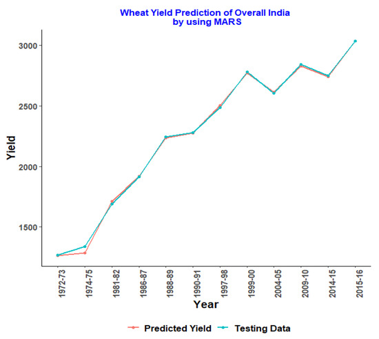
Figure 1.
MARS model for overall India.
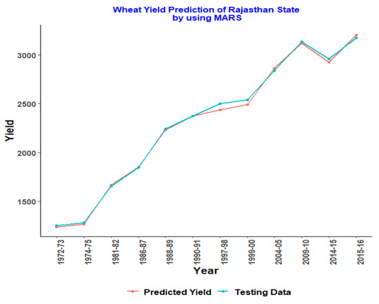
Figure 2.
MARS model for Rajasthan.
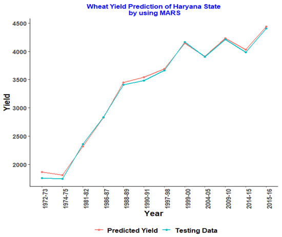
Figure 3.
MARS model for Haryana.
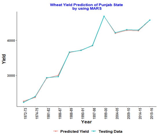
Figure 4.
MARS model for Punjab.
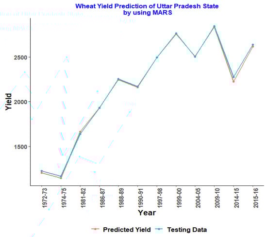
Figure 5.
MARS model for Uttar Pradesh.
4. Conclusions
Machine learning methods have gained popularity across a broad spectrum of applications, and they have been proven to be effective in agrarian research. Crop yield prediction is significant in many parts of the country’s economy since it provides data for decision-making. A PCA-based MARS model was implemented to study wheat data and predict yield for overall India and the major wheat-producing states. The findings indisputably established that the MARS model has a better fit and was functional for studying the complex non-linear relationships. Further investigation can be carried out into this study considering various other parameters such as climatic factors, irrigation, and the different types of fertilizers. Several studies have found that models with more features do not produce accurate predictions and vary depending on the context. Models with more and fewer characteristics can be examined to determine the best-performing model. However, the results clearly show that when used in agricultural yield prediction, machine learning models such as MARS outperform traditional statistical models.
Author Contributions
Conceptualization, B.M.N., K.R.K. and C.C.; methodology, B.M.N., K.R.K. and C.C.; validation, B.M.N., K.R.K. and C.C.; formal analysis, B.M.N., K.R.K. and C.C.; investigation, B.M.N., K.R.K. and C.C.; writing—original draft preparation, B.M.N., K.R.K. and C.C.; writing—review and editing, B.M.N., K.R.K. and C.C. All authors have read and agreed to the published version of the manuscript.
Funding
This research received no external funding.
Institutional Review Board Statement
Not applicable.
Informed Consent Statement
Not applicable.
Data Availability Statement
The data that support the findings of this study are available from the corresponding author upon reasonable request.
Conflicts of Interest
The authors declare no conflict of interest.
References
- Ali, J. Livestock sector development and implications for rural poverty alleviation in India. Livest. Res. Rural Dev. 2007, 19, 1–15. [Google Scholar]
- Premanandh, J. Factors affecting food security and contribution of modern technologies in food sustainability. J. Sci. Food Agric. 2011, 91, 2707–2714. [Google Scholar] [CrossRef] [PubMed]
- Palanivel, K.; Surianarayanan, C. An approach for prediction of crop yield using machine learning and big data techniques. Int. J. Comput. Eng. Technol. 2019, 10, 110–118. [Google Scholar] [CrossRef]
- Ju, S.; Lim, H.; Heo, J. Machine learning approaches for crop yield prediction with MODIS and weather data. In Proceedings of the 40th Asian Conference on Remote Sensing: Progress of Remote Sensing Technology for Smart Future, ACRS 2019, Daejeon, Korea, 14–18 October 2019. [Google Scholar]
- Paudel, D.; Boogaard, H.; de Wit, A.; Janssen, S.; Osinga, S.; Pylianidis, C.; Athanasiadis, I.N. Machine learning for large-scale crop yield forecasting. Agric. Syst. 2021, 187, 103016. [Google Scholar] [CrossRef]
- Rashid, M.; Bari, B.S.; Yusup, Y.; Kamaruddin, M.A.; Khan, N. A Comprehensive Review of Crop Yield Prediction Using Machine Learning Approaches with Special Emphasis on Palm Oil Yield Prediction. IEEE Access 2021, 9, 63406–63439. [Google Scholar] [CrossRef]
- Aslam, F.; Salman, A.; Jan, I. Predicting Wheat Production in Pakistan by using an Artificial Neural Network Approach. Sarhad J. Agric. 2019, 35, 1054–1062. [Google Scholar] [CrossRef]
- Stas, M.; Van Orshoven, J.; Dong, Q.; Heremans, S.; Zhang, B. A comparison of machine learning algorithms for regional wheat yield prediction using NDVI time series of SPOT-VGT. In Proceedings of the 2016 Fifth International Conference on Agro-Geoinformatics (Agro-Geoinformatics), Tianjin, China, 18–20 July 2016; pp. 1–5. [Google Scholar]
- Heremans, S.; Dong, Q.; Zhang, B.; Bydekerke, L.; Van Orshoven, J. Potential of ensemble tree methods for early-season prediction of winter wheat yield from short time series of remotely sensed normalized difference vegetation index and in situ meteorological data. J. Appl. Remote Sens. 2015, 9, 097095. [Google Scholar] [CrossRef]
- Li, Z.; Wang, J.; Tang, H.; Huang, C.; Yang, F.; Chen, B.; Wang, X.; Xin, X.; Ge, Y. Predicting Grassland Leaf Area Index in the Meadow Steppes of Northern China: A Comparative Study of Regression Approaches and Hybrid Geostatistical Methods. Remote Sens. 2016, 8, 632. [Google Scholar] [CrossRef]
- Han, J.; Zhang, Z.; Cao, J.; Luo, Y.; Zhang, L.; Li, Z.; Zhang, J. Prediction of Winter Wheat Yield Based on Multi-Source Data and Machine Learning in China. Remote Sens. 2020, 12, 236. [Google Scholar] [CrossRef]
- Paidipati, K.K.; Chesneau, C.; Nayana, B.M.; Kumar, K.R.; Polisetty, K.; Kurangi, C. Prediction of Rice Cultivation in India—Support Vector Regression Approach with Various Kernels for Non-Linear Patterns. AgriEngineering 2021, 3, 182–198. [Google Scholar] [CrossRef]
- Joshua, V.; Priyadharson, S.M.; Kannadasan, R. Exploration of Machine Learning Approaches for Paddy Yield Prediction in Eastern Part of Tamilnadu. Agronomy 2021, 11, 2068. [Google Scholar] [CrossRef]
- Kassambara, A. Machine Learning Essentials: Practical Guide in R; CreateSpace: Scotts Valley, CA, USA, 2017. [Google Scholar]
- Nisbet, R.; Elder, J.; Miner, G. Handbook of Statistical Analysis and Data Mining Applications; Academic Press: Cambridge, MA, USA, 2009. [Google Scholar]
- Tyasi, T.L.; Makgowo, K.M.; Mokoena, K.; Rashijane, L.T.; Mathapo, M.C.; Danguru, L.W.; Molabe, K.M.; Bopape, P.M.; Mathye, N.D.; Maluleke, D. Multivariate Adaptive Regression Splines Data Mining Algorithm for Prediction of Body Weight of Hy-Line Silver Brown Commercial Layer Chicken Breed. Adv. Anim. Vet. Sci. 2020, 8, 794–799. [Google Scholar] [CrossRef]
- Turpin, K.M.; Lapen, D.R.; Gregorich, E.G.; Topp, G.C.; Edwards, M.; McLaughlin, N.B.; Robin, M.J.L. Using multivariate adaptive regression splines (MARS) to identify relationships between soil and corn (Zea mays L.) production properties. Can. J. Soil Sci. 2005, 85, 625–636. [Google Scholar] [CrossRef]
- Eyduran, E.; Akin, M.; Eyduran, S.P. Application of multivariate adaptive regression splines in agricultural sciences through R Software. Nobel Bilimsel Eser. Sertifika 2019, 20779. [Google Scholar]
- Ferreira, L.B.; Duarte, A.B.; Cunha, F.F.D.; Fernandes, E.I. Multivariate adaptive regression splines (MARS) applied to daily reference evapotranspiration modeling with limited weather data. Acta Scientiarum. Agron. 2019, 41, 39880. [Google Scholar] [CrossRef]
- Celik, S.; Boydak, E. Description of the relationships between different plant characteristics in soybean using multivariate adaptive regression splines (MARS) algorithm. JAPS J. Anim. Plant Sci. 2020, 30, 431–441. [Google Scholar]
- Adler, K.; Piikki, K.; Söderström, M.; Eriksson, J.; Alshihabi, O. Predictions of Cu, Zn, and Cd Concentrations in Soil Using Portable X-Ray Fluorescence Measurements. Sensors 2020, 20, 474. [Google Scholar] [CrossRef]
- Elith, J.; Leathwick, J. Predicting species distributions from museum and herbarium records using multiresponse models fitted with multivariate adaptive regression splines. Divers. Distrib. 2007, 13, 265–275. [Google Scholar] [CrossRef]
- Msilini, A.; Masselot, P.; Ouarda, T.B. Regional Frequency Analysis at Ungauged Sites with Multivariate Adaptive Regression Splines. J. Hydrometeorol. 2020, 21, 2777–2792. [Google Scholar] [CrossRef]
- Canga, D. Use of Mars Data Mining Algorithm Based on Training and Test Sets in Determining Carcass Weight of Cattle in Different Breeds. J. Agric. Sci. 2022, 28, 259–268. [Google Scholar]
- Oduro, S.D.; Metia, S.; Duc, H.; Hong, G.; Ha, Q. Multivariate adaptive regression splines models for vehicular emission prediction. Vis. Eng. 2015, 3, 13. [Google Scholar] [CrossRef]
- Jolliffe, I.T.; Cadima, J. Principal component analysis: A review and recent developments. Philos. Trans. R. Soc. A Math. Phys. Eng. Sci. 2016, 374, 20150202. [Google Scholar] [CrossRef] [PubMed]
- Paul, L.C.; Suman, A.A.; Sultan, N. Methodological analysis of principal component analysis (PCA) method. Int. J. Comput. Eng. Manag. 2013, 16, 32–38. [Google Scholar]
- Friedman, J.H. Multivariate adaptive regression splines. Ann. Stat. 1991, 19, 1–67. [Google Scholar] [CrossRef]
- Friedman, J.H.; Roosen, C.B. An introduction to multivariate adaptive regression splines. Stat. Methods Med. Res. 1995, 4, 197–217. [Google Scholar] [CrossRef] [PubMed]
- Amin, M.M.; Zainal, A.; Azmi, N.F.M.; Ali, N.A. Feature Selection Using Multivariate Adaptive Regression Splines in Telecommunication Fraud Detection. In IOP Conference Series: Materials Science and Engineering; IOP Publishing: Bristol, UK, 2020; Volume 864, p. 012059. [Google Scholar]
- Ramadas, S.; Kumar, T.K.; Singh, G.P. Wheat production in India: Trends and prospects. In Recent Advances in Grain Crops Research; IntechOpen: London, UK, 2020. [Google Scholar]


Publisher’s Note: MDPI stays neutral with regard to jurisdictional claims in published maps and institutional affiliations. |
© 2022 by the authors. Licensee MDPI, Basel, Switzerland. This article is an open access article distributed under the terms and conditions of the Creative Commons Attribution (CC BY) license (https://creativecommons.org/licenses/by/4.0/).