Abstract
Bird welfare and comfort is highly impacted by extreme environments, including hot/cold temperatures, relative humidity, and heat production within the coops during loading at the farm, transportation, and holding at the processing plants. Due to the complexity of the multiphysics phenomena involving fluid flow, heat transfer, and multispecies mixtures (humidity) within the coops, machine learning models may be helpful to evaluate broiler welfare under various environments. Machine learning techniques (Artificial Neural Networks and Bayesian Optimization) were applied to estimate the desired parameters required to ensure broiler welfare inside the coops. Artificial Neural Networks (ANNs) were trained with the results of Computational Fluid Dynamics (CFD) simulations for various ranges of inputs related to the microenvironment. Input variables included air velocity, broiler heat production, ambient temperature, and relative humidity. The Output variable was the Enthalpy Comfort Index (ECI), which is a measure of the bird welfare. The trained networks were then analyzed using Bayesian Optimization (BO) for the inverse mapping of ANNs and to predict the range of acceptable input parameters for a desired output, i.e., ECI in the comfort level. Results indicate that reducing the broilers heat production inside the coop along with increasing fan velocity enhances the broiler welfare and the thermal microenvironment. The BO developed in this study provide the microenvironmental parameters to estimate the bird welfare that is comfortable.
1. Introduction
Bird welfare and comfort is highly impacted by extreme environments (ambient temperature, relative humidity, and heat production by the bird within the poultry coop) during loading at the farm, transportation, and holding at the processing plants. The birds can be exposed to extremes of temperature and humidity during transportation, especially during the summer months and these conditions are a major cause for dead birds on arrival (DOAs) [1,2]. In the hot temperature environment, the broiler is unable to efficiently lose the produced heat (generated within the bird), resulting in an increase in its body temperature which could be fatal and/or reduce the meat quality [3]. Use of fans along with surface wetting of the birds (evaporative cooling) are among the promising approaches for reducing the body temperature and dealing with the thermal discomfort [4,5,6].
Computational Fluid Dynamics (CFD) simulations have been applied for better understanding the effects of various parameters on the bird welfare [7,8,9,10,11,12]. Heymsfield et al. [9] simulated the air velocity distribution inside coops but did not consider the impact of ambient relative humidity and the bird heat production. Pawar et al. [11] included the heat production by the birds to investigate different ventilation schemes via a 2-D CFD model; however, the ambient relative humidity was not studied. Shivkumar et al. [12] incorporated the bird’s heat flux in their 3-D model, yet the ambient relative humidity was not considered. Recently, we conducted 3-D CFD simulations to study the effects of the ambient temperature and relative humidity along with the bird heat production on the thermal microenvironment inside poultry coops [13]. While CFD simulations provide insight on the impacts of various parameters on the microenvironment, they fall short in estimating the range of acceptable input parameters to acquire the optimal microenvironment condition in the coops. The parameter estimation is an optimization problem, where the parameters are adjusted in a way to minimize a function (in this case the difference between the microenvironment and the desired conditions). Machine learning methods have been widely used to solve optimizations problem and have been the subject of various studies in agricultural engineering in the past decade for applications including, but not limited to, optimal lighting control in the greenhouse [14,15], irrigation management [16], estimation of wheat yield [17], classification of the ripeness of mango fruit [18], and disease detection in wheat [19], as well as prediction of the behavior pattern and health of broiler chicken [20,21,22]. Despite the ever-growing application of machine learning in agricultural research, to the best of our knowledge, it has not been used in any previous study for the broiler welfare inside poultry coops. This is especially important given that various parameters such as air velocity and heat production by the birds, as well as ambient temperature and relative humidity, affect the microenvironment inside the coops and the bird’s welfare. In the current study we applied machine learning to estimate the range of acceptable input parameters that ensure bird welfare.
In this context, we trained shallow Artificial Neural Networks (ANNs) that map the input parameters to the bird welfare index using the data from our CFD simulations results from our previous work [13]. The trained network was then used for the inverse mapping using Bayesian Optimization (BO) to estimate the range of input parameters for a desired broiler comfort state.
The remainder of this paper is organized as follows. The method, CFD model, and the machine learning methods, i.e., ANN and the inverse mapping using BO are discussed in Section 2. Section 3 presents the results for a typical bird welfare optimization problem. The conclusions from this study are presented in Section 4.
2. Methodology
The poultry coops are loaded with broilers on the farm, stacked on a trailer, transported to the processing plant and are parked in holding sheds as shown in Figure 1. These holding sheds are equipped with fans to blow air to improve the immediate bird environment inside the coop. Temperature and relative humidity are the two significant environmental parameters that determine the broilers welfare inside the coop. The combined effects of both temperature and relative humidity are often used to evaluate the bird welfare via an integrated comfort index called Enthalpy Comfort Index [23,24]. In this context, Enthalpy Comfort Index (ECI) is defined as:
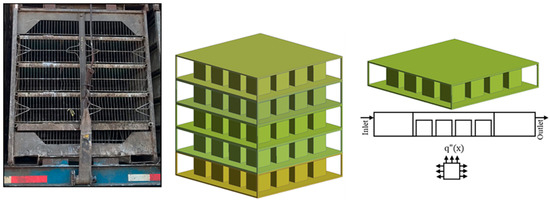
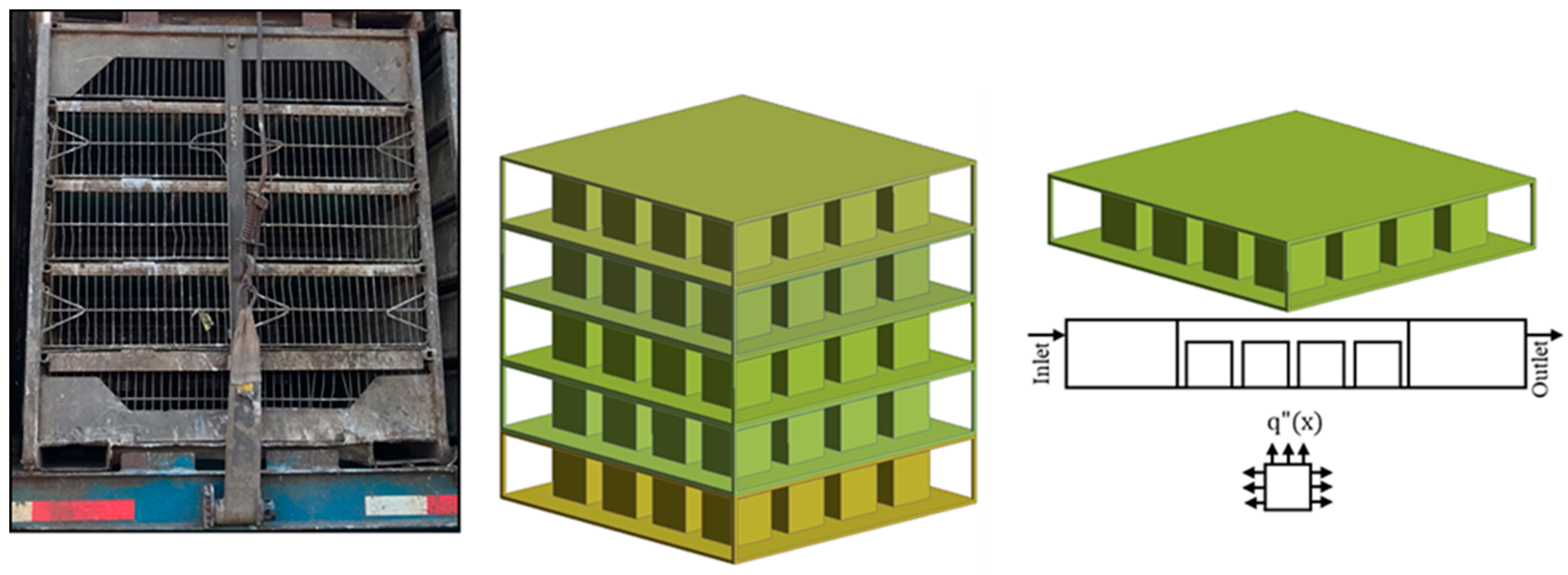
Figure 1.
The stacks of poultry coops on a trailer, and the 3-D model for a single coop. Cubes represent broilers.
Here, is the temperature in Celsius, RH is the relative humidity percentage, and is the barometric pressure in mmHg [23]. The ECI in the ranges of ECI ≤ 48 kJ/kg, 48.1 ≤ ECI ≤ 57.6 kJ/kg, 57.7 ≤ ECI ≤ 66.1 kJ/kg, and 66.2 ≤ ECI kJ/kg are considered to be in the comfort, warning, critical, and lethal region, respectively.
Equation (1), despite being a powerful tool to estimate the welfare of the broilers using two most important parameters (i.e., ambient temperature and relative humidity), is not capable of distinguishing between the bird welfare along the length of the coop (fan side, center, or far from the fan). Typically, due to the heat production by the birds, birds located at the center and downstream of the coop experience more thermal discomfort compared to those near the fan (inlet). In the absence of experimental data, we applied computational fluid dynamics (CFD) simulations to model the immediate bird environment inside the coop via calculating a microenvironment metric (ECI) and using this metric in the machine learning model (Artificial Neural Networks and Bayesian Optimization). The CFD model [13], ANN model, and Bayesian optimization are presented below.
2.1. CFD Model
In the simulations, air was blown from the inlet and passed through the coop. Despite the fact that the simulations could be conducted for any number of birds, for the sole purpose of a parametric study, the coop was assumed to be loaded with 16 broilers each weighing 2.5 kg. For the sake of geometry and mesh simplicity, the wire meshing and metal supports on the side faces were excluded and broilers were modeled as cubes with surface area similar to that for 2.5 kg broilers [25]. Ansys Fluent 2020 R2 was utilized to conduct the CFD simulations, where a steady state 3-D model was considered for the humid air flow (humidity modeled by species transport model). The length, width, and height of the coop considered in this study were 1.19, 1.17, and 0.25 m, respectively. Velocity inlet boundary condition was assigned at the inlet, and the flow velocity was varied in the range of . The Reynolds numbers were in the order of magnitude of O(104–105) and the flow was hence turbulent. A turbulence model was used for the simulations, which added the following two equations, Equations (2) and (3), for the turbulent kinetic energy (k), and the turbulent dissipation rate (ε).
Here, is the turbulent (eddy) viscosity and is the generation of turbulent kinetic energy computed as:
The following values were considered for the empirical constants:
The standard wall function was utilized to resolve the viscous sub-layer. No slip boundary condition was assumed for all the walls (coop and bird). The coop walls were considered adiabatic, having zero heat flux, while heat flux in the range of 0–300 was assigned to the birds’ wall (to consider the broilers heat production). Various ambient temperature and relative humidity values in the range of , and were assigned at the inlet. Pressure outlet boundary condition with a zero-gauge pressure is assumed at the outlet. Symmetry boundary condition was defined for the left and right sides of the domain. A structured mesh was used in this work, and finer mesh was selected in the regions adjacent to the walls. A mesh independency study was conducted over five different grid resolutions and a total of 470,500 hexahedral elements with 510,346 nodes were selected (see Figure 2).
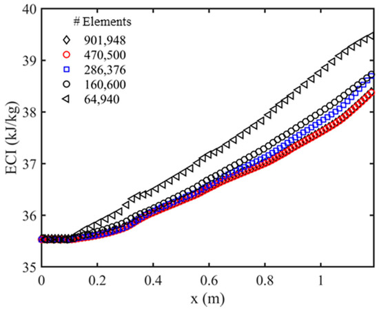
Figure 2.
The mesh independency analysis by calculating ECI along x-axis for an ambient temperature of 300 k, relative humidity of 15%, the broilers heat production of 150 and air velocity of 0.5 m/s.
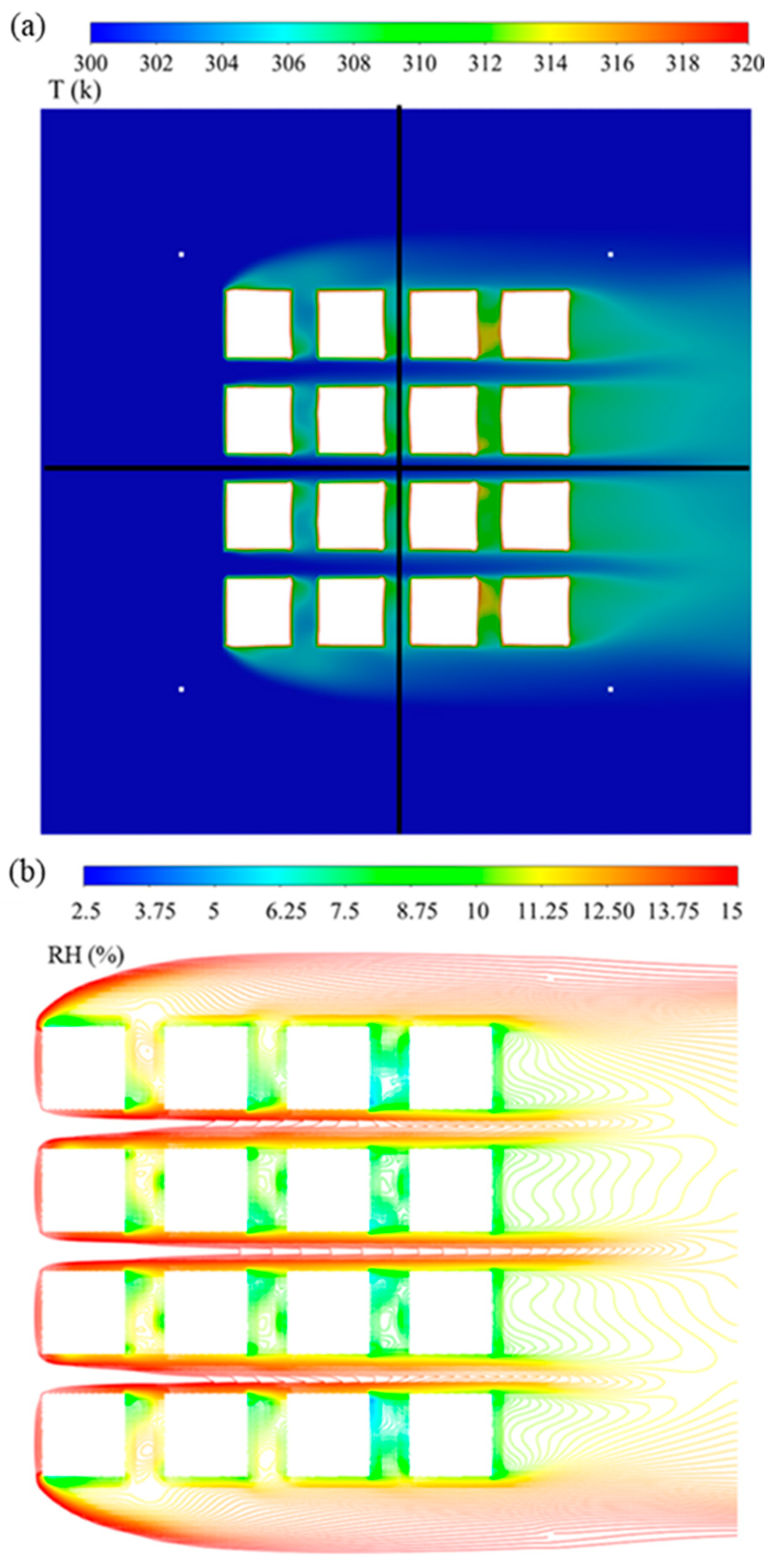
The CFD model in Ansys Fluent solved the conservation equations (conservation of mass, momentum, energy, mass fraction of species, and turbulence parameters) subjected to the boundary conditions until it reached the convergence. The solution convergence was judged by monitoring the residual to ensure that solution does not change subsequent iterations and has almost zero heat/mass imbalance. The CFD model was discussed in detail in our recent study [13]. The CFD solution produces temperature and relative humidity maps, showing the spatially varying values for both variables inside the coops (see Figure 3).
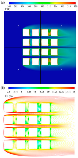
Figure 3.
Contours of (a) temperature and (b) relative humidity are shown on the horizontal plane at the mid height of the coop for the simulation with an inlet velocity of 0.5 m/s, relative humidity of 15%, and the temperature of 300 k.
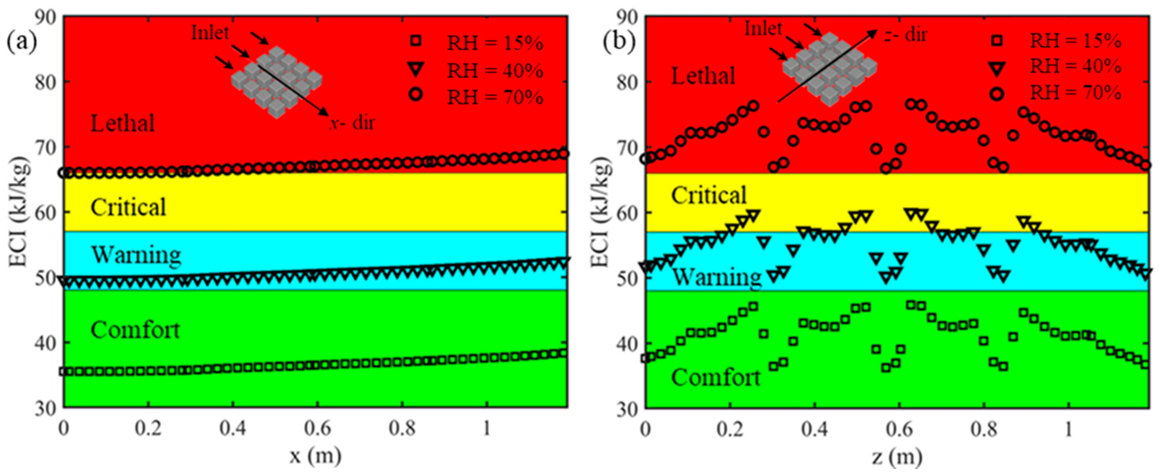
In our study, local (rather than ambient) temperature and relative humidity (the outputs of the CFD simulations) were applied in Equation (1), which results in a range of ECI values. The variation of the ECI along the longitudinal and transverse direction of the coop (i.e., x, and z-dir.) is shown in Figure 4.

Figure 4.
Effects of inlet air relative humidity on the enthalpy comfort index for inlet velocity of 0.5 m/s, inlet temperature of 300 k, and the broilers heat production of 150 along (a) x-direction and (b) z-direction.
2.2. Optimization Using Machine Learning
The maximum value of the ECI inside the coop was then selected for the design (optimization) problem. In this section, we applied machine learning techniques to the results of the CFD simulations to find a relationship between the maximum ECI and air velocity, bird heat production, ambient temperature, and relative humidity as .
2.2.1. Artificial Neural Network (ANN) Model
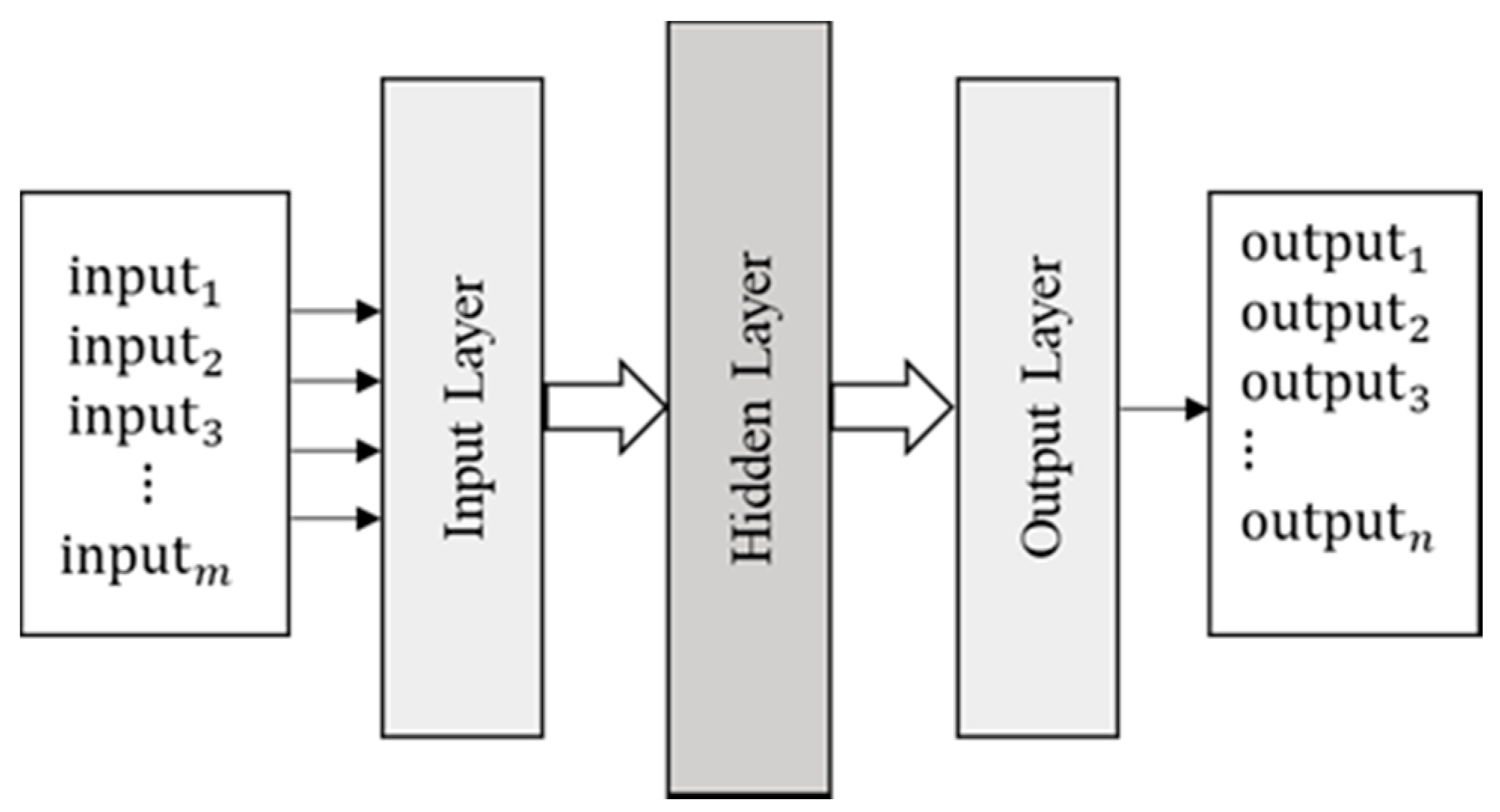
ANNs are statistical models used to find non-linear relations between input data () and outputs (). In other words, ANN is a process of estimating the function that maps inputs to the outputs, i.e., . In general, the input and outputs can be vectors of lengths m, and n (m, n), i.e., , and as shown in Figure 5.
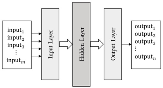
Figure 5.
Architecture of the ANNs, consisting of the input, hidden, and output layer.
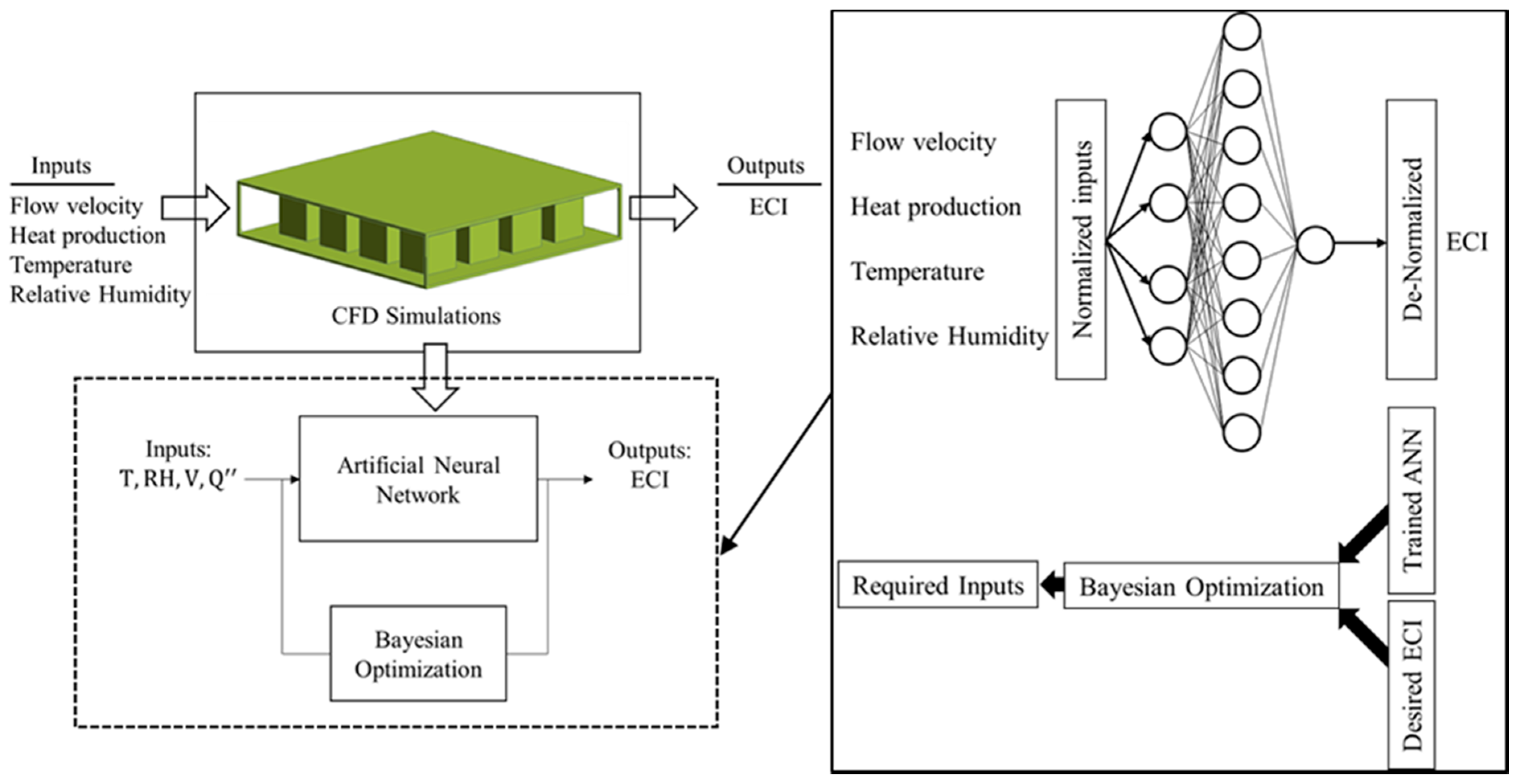
In the CFD analysis, there are four major input parameters, i.e., air velocity, heat production, ambient temperature, relative humidity () and one output parameter, i.e., ECI (). Note that the ambient pressure is often a constant value (1 atm) and is not considered as an individual input parameter in this study. The shallow ANNs (network with a single hidden layer) with eight hidden neurons were trained with 108 training examples obtained from CFD simulations. The training examples were randomly split in a way that 70%, 15%, and 15% of the dataset was assigned for training, validating, and testing the network, respectively. The architecture of the ANNs used for the training is illustrated in Figure 6.
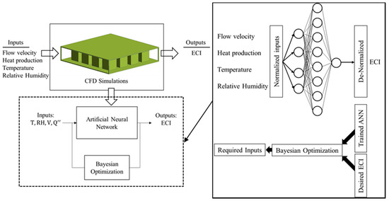
Figure 6.
Integration of the CFD model with the machine learning to estimate the range of acceptable input parameters.
Ten different ANNs were trained in this study, and the best performer was selected for the inverse mapping problem.
2.2.2. Inverse Mapping of the ANNs Using Bayesian Optimization
Consider an optimization problem where we are interested in knowing the range of heat production and inlet velocity parameters required to obtain a desired thermal comfort level ECI0 (ECI0 ≤ 48 kJ/kg) for the birds in an ambient temperature and relative humidity of T0 and RH0. In order to find an explicit equation between the optimization ECI and input parameters like , shallow ANNs with eight hidden neurons were fitted to our CFD data. MATLAB’s tansig transfer function was used as the activation function in the hidden layer. Upon mathematical computation of the weight, bias, and activation functions of the trained network (best performer), the is calculated as:
with the being calculated from Table 1. This equation explicitly maps the input parameters () to the output (), which simplifies the optimization problem. To get the desired comfort index of (output), for a specific ambient condition (), one can plug these values into Equation (6) to have:

Table 1.
The coefficients for calculating the .
Equation (7) becomes a problem of finding roots for that satisfies , which can be solved using any traditional root finding approaches. In this study, we applied the Bayesian Optimization (BO) to minimize which ultimately gives the roots. BO is a learning algorithm for finding the minimum of an objective function (cost function) . BO is performed by first initializing a Gaussian Process ‘surrogate function’ prior distribution, and then selecting several data points x in a way that maximizes the acquisition function a(x) operating on the current prior distribution. The data points x in the objective cost function are then evaluated and the results, y, are obtained and added to the data set and the Gaussian Process prior distribution will be updated with the new data to produce a posterior (basically the prior in the next step). The above-mentioned steps were repeated over several iterations. Ultimately the global minima were found by interpreting the current Gaussian Process distribution. The Bayesian Optimization function of bayesopt in MATLAB R2020b was used in this study, which considers the acquisition function of expected improvement [26].
3. Results and Discussion
The shallow neural networks with eight hidden neurons perfectly fit the training data set (70% of the data; Figure 7a) where the data lie on a line with a slope of R = 0.99951 (the 45° line) in the output vs. target plot. It is also worth mentioning that the ANNs work precisely for other data sets as well, e.g., the fit to the validation, test, and all datasets are shown in Figure 7b–d, respectively. This proves the fact that shallow ANNs can perfectly map the inputs to the output without any bias or variance problem.
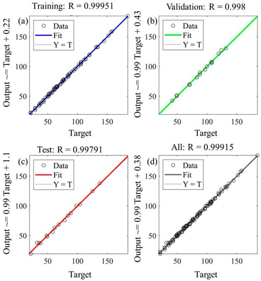
Figure 7.
The regression plot to show the accuracy of the ANN in fitting to data in the, (a) training, (b) validation, (c) test, and (d) all datasets.
Figure 8a shows the error histogram illustrating the performance of the networks. It is shown that most datasets lay near the zero-error point, where target equals the output values, and only few instances are away from this point with maximum error being negligible compared to range of ECIs (30–160). The performance of the ANN is shown in terms of the Mean Squared Error (MSE) in Figure 8b. As shown in this figure, the MSE keeps decreasing with each training cycle (epoch), until it converges and reaches a minimum value for the validation datasets.
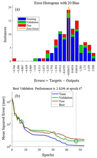
Figure 8.
The performance of the ANN on the training, validation, and test datasets are depicted in terms of (a) the error histogram and (b) the MSE during various training cycles.
For the sole purpose of demonstrating the accuracy of the ANN prediction, we considered a case with an inlet velocity of , temperature of , relative humidity of , and a heat production of . Each of these input values were different from those used to train the ANN which results in unbiased predictions (in addition to the test set regression plot shown in Figure 7c). The trained ANN predicts a maximum comfort index value of . After conducting the CFD simulations for those input conditions the was computed, which shows a reasonable accuracy for the ANNs prediction.
As discussed earlier, the inverse mapping was conducted using the bayesopt function in MATLAB. The results of the CFD simulations show that increasing ambient temperature and/or relative humidity results in an increase in ECI, and unfavorable bird welfare (distress). It is also known from CFD simulation that increasing the bird heat production results in higher ECI. A similar trend was observed from the BO inverse mapping as seen in Table 2. Note that to estimate each of the input parameters (e.g., T) via the BO, one needs to plug the known values for other parameters (i.e., and ) into Equation (6) and solve for the unknown parameter.
Table 2.
Results of BO inverse mapping to obtain ambient relative humidity and temperature for various .
Table 3 estimates the velocity and heat production for various broilers welfare conditions on a typical day with ambient temperature of 300 k and relative humidity of 15%.
Table 3.
Results of BO inverse mapping to estimate input parameters for and various = 43 (comfort); 53 (warning); 63 (critical); and 73 (lethal).
For the inverse mapping, one can specify any combinations of inputs and estimate the other inputs. Table 4 estimates various input parameters for different welfare conditions.
Table 4.
Results of BO inverse mapping to estimate input parameters for various .
The accuracy of the inverse mapping using BO is shown here by considering one of the cases in Table 4, where at an inlet velocity of and temperature of , for the broilers to be in a critical welfare condition (with ) the BO predicts the relative humidity of , and a heat production of . Performing CFD simulations for these input parameters () results in a maximum comfort index of , which has less than 3% difference with the objective
The birds are loaded in the coops at the farm, transferred to the trailer, transported to the processing facility, and held in holding sheds until processing. At the farm and in the holding sheds at the processing facility, fans are provided to blow air through the coops to reduce the temperature and, in some cases, the humidity (water vapor) within the coop—both generated by the bird. However, under extreme environmental conditions prevalent during the summer months in Southeast U.S., Moghadam et al. [13] showed that blowing air using the fans alone is not adequate to assure bird welfare (as indicated by the ECI). Using the ANN approach, we were able to show that under extreme environmental conditions (high temperate and humidity), the bird welfare can be assured by decreasing the heat produced by the birds. Alternatively, for a given heat flux per bird this can be done by decreasing the number of birds loaded on to the coop. This may be a practical approach to minimize the bird mortality and other meat quality-related issues that reduce the value of the broiler meat and the resulting economic loss for the processor. Another important problem is finding the airflow velocity that assures welfare for increasing number of birds. To investigate this problem, we applied BO on the ANN model for cases with a fixed ambient temperature and relative humidity of 300 k and 15%, but with heat generation in the range of 100–250 to find the velocity that assures the bird welfare with ECI = 45 kJ/kg (see Table 5).
Table 5.
Results of BO inverse mapping to estimate velocity to ensure comfort for various heat production for and = 45 (comfort).
It is seen that larger airflow velocity is needed to assure comfort for an increasing number of birds, which is implicitly represented by increasing heat flux in our study. An explicit prediction of the maximum number of birds that needs to be loaded in the coop to assure bird comfort for a particular set of environmental conditions (temperature, humidity, and maximum air velocity) can be accomplished by conducting CFD simulations with similar environmental conditions and fan velocity, but various numbers of birds per coops and calculating the , which could be the subject of a future study.
4. Conclusions
Machine learning techniques were applied to estimate the optimal conditions required for ensuring bird welfare and thermal microenvironment inside the poultry coops. Simulation results of a CFD model for a loaded poultry coop were applied to train the simple, yet highly efficient shallow ANNs which found a nonlinear mathematical equation between the input (flow velocity, broiler heat production, ambient temperature, and relative humidity) and the output (ECI) parameters. The inverse mapping of the trained ANNs was then performed via BO method to estimate the range of acceptable parameters that result in a comfort region in the entire coop microenvironment. The results show that the bird welfare can be improved by reducing the number of birds in the coop, along with increasing the air flow velocity. The results also show that the BO can be utilized to investigate the combined effects of parameters, such as estimating the extent to which the airflow needs to be increased to assure welfare for an increasing number of birds. This information might be useful for poultry industries.
Author Contributions
Conceptualization, R.P.; methodology, A.M., R.P. and H.T.; implementation, A.M.; writing—original draft, A.M.; review and editing, R.P. and H.T.; project administration, R.P. and H.T. All authors have read and agreed to the published version of the manuscript.
Funding
This research was supported by USDA, National Institute of Food and Agriculture under award 2020-67015-31915.
Institutional Review Board Statement
Not applicable.
Informed Consent Statement
Not applicable.
Data Availability Statement
The data presented in this study are available on request from the corresponding author.
Acknowledgments
This material is based on work that is supported by the USDA, National Institute of Food and Agriculture under award 2020-67015-31915. Mention of trade names or commercial products in this publication is solely for the purpose of providing scientific information and does not imply recommendation or endorsement by the USDA or the University of Georgia, Athens.
Conflicts of Interest
The authors declare no conflict of interest.
References
- Hoxey, R.P.; Kettlewell, P.J.; Meehan, A.M.; Baker, C.J.; Yang, X. An investigation of the aerodynamic and ven-tilation characteristics of poultry transport vehicles: Part I, full-scale measurements. J. Agric. Eng. Res. 1996, 65, 77–83. [Google Scholar] [CrossRef]
- Kettlewell, P.J.; Mitchell, M.A. Mechanical ventilation: Improving the welfare of broiler chickens in transport. J. R. Agric. Soc. Engl. 2001, 162, 175–184. [Google Scholar]
- Schwartzkopf-Genswein, K.; Faucitano, L.; Dadgar, S.; Shand, P.; Gonzalez, L.; Crowe, T. Road transport of cattle, swine and poultry in North America and its impact on animal welfare, carcass and meat quality: A review. Meat Sci. 2012, 92, 227–243. [Google Scholar] [CrossRef] [PubMed]
- Aldridge, D.J.; Luthra, K.; Liang, Y.; Christensen, K.; Watkins, S.E.; Scanes, C.G. Thermal Micro-Environment during Poultry Transportation in South Central United States. Animals 2019, 9, 31. [Google Scholar] [CrossRef] [PubMed] [Green Version]
- Liang, Y.; Tabler, G.T.; Costello, T.A.; Berry, I.L.; Watkins, S.E.; Thaxton, Y.V. Cooling broiler chickens by surface wetting: Indoor thermal environment, water usage, and bird performance. Appl. Eng. Agric. 2014, 30, 249–258. [Google Scholar]
- Tao, X.; Xin, H. Surface wetting and its optimization to cool broiler chickens. Trans. ASAE 2003, 46, 483. [Google Scholar] [CrossRef]
- Bustamante, E.; García-Diego, F.J.; Calvet, S.; Estellés, F.; Beltrán, P.; Hospitaler, A.; Torres, A.G. Exploring venti-lation efficiency in poultry buildings: The validation of computational fluid dynamics (CFD) in a cross-mechanically ventilated broiler farm. Energies 2013, 6, 2605–2623. [Google Scholar] [CrossRef] [Green Version]
- Gilkeson, C.; Thompson, H.; Wilson, M.; Gaskell, P. Quantifying passive ventilation within small livestock trailers using Computational Fluid Dynamics. Comput. Electron. Agric. 2016, 124, 84–99. [Google Scholar] [CrossRef] [Green Version]
- Heymsfield, C.L.; Liang, Y.; Costello, T.A. Computational Fluid Dynamics Model of Air Velocity through a Poultry Transport Trailer in a Holding Shed. Appl. Eng. Agric. 2020, 36, 963–973. [Google Scholar] [CrossRef]
- Norton, T.; Kettlewell, P.; Mitchell, M. A computational analysis of a fully-stocked dual-mode ventilated livestock vehicle during ferry transportation. Comput. Electron. Agric. 2013, 93, 217–228. [Google Scholar] [CrossRef]
- Pawar, S.R.; Cimbala, J.M.; Wheeler, E.F.; Lindberg, D.V. Analysis of Poultry House Ventilation Using Computational Fluid Dynamics. Trans. ASABE 2007, 50, 1373–1382. [Google Scholar] [CrossRef]
- Shivkumar, A.P.; Li, L.; Shah, S.B.; Stikeleather, L.; Fuentes, M. Performance Analysis of a Poultry Engineering Chamber Complex for Animal Environment, Air Quality, and Welfare Studies. Trans. ASABE 2016, 59, 1371–1381. [Google Scholar] [CrossRef]
- Moghadam, A.; Thippareddi, H.; Regmi, P.; Pidaparti, R. Modeling and Simulation of the Microenvironment in the Poultry Coops. J. ASABE 2022. [Google Scholar] [CrossRef]
- Afzali, S.; Mosharafian, S.; van Iersel, M.W.; Mohammadpour Velni, J. Development and Implementation of an IoT-Enabled Optimal and Predictive Lighting Control Strategy in Greenhouses. Plants 2021, 10, 2652. [Google Scholar] [CrossRef] [PubMed]
- Mosharafian, S.; Afzali, S.; Weaver, G.M.; van Iersel, M.; Velni, J.M. Optimal lighting control in greenhouse by incorporating sunlight prediction. Comput. Electron. Agric. 2021, 188, 106300. [Google Scholar] [CrossRef]
- Abioye, E.A.; Hensel, O.; Esau, T.J.; Elijah, O.; Abidin, M.S.Z.; Ayobami, A.S.; Nasirahmadi, A. Precision Irri-gation Management Using Machine Learning and Digital Farming Solutions. AgriEngineering 2022, 4, 70–103. [Google Scholar] [CrossRef]
- Astaoui, G.; Dadaiss, J.; Sebari, I.; Benmansour, S.; Mohamed, E. Mapping Wheat Dry Matter and Nitrogen Content Dynamics and Estimation of Wheat Yield Using UAV Multispectral Imagery Machine Learning and a Variety-Based Approach: Case Study of Morocco. AgriEngineering 2021, 3, 29–49. [Google Scholar] [CrossRef]
- Worasawate, D.; Sakunasinha, P.; Chiangga, S. Automatic Classification of the Ripeness Stage of Mango Fruit Using a Machine Learning Approach. AgriEngineering 2022, 4, 32–47. [Google Scholar] [CrossRef]
- Xie, Y.; Plett, D.; Liu, H. Detecting Crown Rot Disease in Wheat in Controlled Environment Conditions Using Digital Color Imaging and Machine Learning. AgriEngineering 2022, 4, 141–155. [Google Scholar] [CrossRef]
- Hepworth, P.J.; Nefedov, A.V.; Muchnik, I.B.; Morgan, K.L.; Akbar, M.; Fraser, A.R.; Graham, G.J.; Brewer, J.M.; Grant, M.H. Broiler chickens can benefit from machine learning: Support vector machine analysis of observational epidemiological data. J. R. Soc. Interface 2012, 9, 1934–1942. [Google Scholar] [CrossRef]
- Branco, T.; Moura, D.; Nääs, I.D.A.; Lima, N.D.S.; Klein, D.; Oliveira, S. The Sequential Behavior Pattern Analysis of Broiler Chickens Exposed to Heat Stress. AgriEngineering 2021, 3, 447–457. [Google Scholar] [CrossRef]
- Milosevic, B.; Ciric, S.; Lalic, N.; Milanovic, V.; Savic, Z.; Omerovic, I.; Doskovic, V.; Djordjevic, S.; Andjusic, L. Machine learning application in growth and health prediction of broiler chickens. World’s Poult. Sci. J. 2019, 75, 401–410. [Google Scholar] [CrossRef]
- Dos Santos, V.M.; Dallago, B.S.L.; Racanicci, A.M.C.; Santana, P.; Cue, R.I.; Bernal, F.E.M. Effect of transportation distances, seasons and crate microclimate on broiler chicken production losses. PLoS ONE 2020, 15, e0232004. [Google Scholar] [CrossRef] [PubMed] [Green Version]
- Rodrigues, V.C.; Da Silva, I.J.O.; Vieira, F.M.C.; Nascimento, S. A correct enthalpy relationship as thermal comfort index for livestock. Int. J. Biometeorol. 2010, 55, 455–459. [Google Scholar] [CrossRef] [PubMed]
- Aerts, J.; Berckmans, D. A virtual chicken for climate control design: Static and dynamic simulations of heat losses. Trans. ASAE 2004, 47, 1765–1772. [Google Scholar] [CrossRef]
- MathWorks Bayesian Optimization Algorithm. 2016. Available online: https://www.mathworks.com/help/stats/bayesian-optimization-algorithm.html#bva8rew-1 (accessed on 20 October 2021).


Publisher’s Note: MDPI stays neutral with regard to jurisdictional claims in published maps and institutional affiliations. |
© 2022 by the authors. Licensee MDPI, Basel, Switzerland. This article is an open access article distributed under the terms and conditions of the Creative Commons Attribution (CC BY) license (https://creativecommons.org/licenses/by/4.0/).