Article

Prediction of Rice Cultivation in India—Support Vector Regression Approach with Various Kernels for Non-Linear Patterns

by
Kiran Kumar Paidipati
1,
Christophe Chesneau
2,*,
B. M. Nayana
3,
Kolla Rohith Kumar
4,
Kalpana Polisetty
5 and
Chinnarao Kurangi
6
1
Department of Statistics, Lady Shri Ram College for Women, University of Delhi, Delhi 110024, India
2
Department of Mathematics, LMNO, Université de Caen-Normandie, Campus II, Science 3, 14032 Caen, France
3
Statistical Investigator, Department of Economics and Statistics, Government of Kerala, Thiruvananthapuram 695033, India
4
Department of Statistics, Pondicherry University, Puducherry 605014, India
5
Division of Mathematics, Department of S and H, Vignan’s Foundation for Science, Technology and Research, Vadlamudi, Guntur, Andhra Pradesh 522213, India
6
Department of Computer Science, Pondicherry University, Puducherry 605014, India
*
Author to whom correspondence should be addressed.
AgriEngineering 2021, 3(2), 182-198; https://doi.org/10.3390/agriengineering3020012
Submission received: 28 February 2021 / Revised: 29 March 2021 / Accepted: 29 March 2021 / Published: 7 April 2021

Abstract

:
The prediction of rice yields plays a major role in reducing food security problems in India and also suggests that government agencies manage the over or under situations of production. Advanced machine learning techniques are playing a vital role in the accurate prediction of rice yields in dealing with nonlinear complex situations instead of traditional statistical methods. In the present study, the researchers made an attempt to predict the rice yield through support vector regression (SVR) models with various kernels (linear, polynomial, and radial basis function) for India overall and the top five rice producing states by considering influence parameters, such as the area under cultivation and production, as independent variables for the years 1962–2018. The best-fitted models were chosen based on the cross-validation and hyperparameter optimization of various kernel parameters. The root-mean-square error (RMSE) and mean absolute error (MAE) were calculated for the training and testing datasets. The results revealed that SVR with various kernels fitted to India overall, as well as the major rice producing states, would explore the nonlinear patterns to understand the precise situations of yield prediction. This study will be helpful for farmers as well as the central and state governments for estimating rice yield in advance with optimal resources.

1. Introduction

Never having any disparity in how it is cooked, boiled, or fried, rice is practically an everyday meal in Indian society, with India being the second-largest rice-producing nation in the world after China. Approximately 90% of the world population in Asia has the consumption of rice in its meal planning [1]. Rice is devoured by a major percentage of the population in India. With a high carbohydrate content, it is an instant energy provider, and as the nation’s populace is growing, being in excess of 400 million throughout the subsequent years, interest in the farming of rice is set to soar.
In India, rice is cultivated in a large portion of the states, with West Bengal leading the way in production, followed by Uttar Pradesh, Andhra Pradesh, Punjab, Tamil Nadu, and Bihar. Rice is a major food grain in India, where the yield is emulous with China, with more than 11% of the global production rate. Rice production has increased 3.5 times during the last 55 years, after the Green Revolution was imposed in India. Nowadays, due to industrialization and improper irrigation facilities, the area under cultivation is declining in many regions of India, decreasing the quantity of rice production as well as the yield. Inordinate rain prompting flooding and dry seasons from unusual warmth waves, notwithstanding the ongoing droop in the economy, has prompted testing conditions for farmers. Hence, accurate rice yield prediction is significant for the food security of India and is as concerning as the mushrooming task in agrarian research. Additionally, early forecasting of the rice yield for adequate information will be considerate to the policy planners and farmers, as well for optimal land utilization and designing economic policies.
Various traditional statistical methods were employed to predict the rice yield based on highly influential parameters, such as the area under cultivation and production, that still resulted in a gap in measuring the accurate information. Advanced machine learning techniques make it possible to implement means of predicting the rice yield by overcoming the limitations of traditional techniques and forecasting methods for current needs. The advantage of machine learning algorithms is their ability to analyze the data through different dimensions, and diverse patterns or relationships can be summarized from the data. Rather than the traditional regression methods, machine learning techniques have the ability to train the models and perform better for the nonlinear data patterns. Since machine learning algorithms are entirely data-driven, they can lessen, if not dispose of, forecaster assumptions and bias. This is exceptionally useful for depicting the nonlinear complex patterns in the prediction of rice yield, making these forecasts more robust. Machine learning techniques are playing a prominent role in dealing with such complex situations and making wise decisions in support of farmers as well as decision-makers.

2. Review of the Literature

Most researchers have focused on developing traditional and advanced regression models in linear and nonlinear situations. Starting with the traditional multiple linear regression to predict the crop yield in Andhra Pradesh [2], kernel ridge, lasso, and elastic net regression models considering parameters such as the state, district, season, area, and year have been used to estimate the particular crop yield in India [3].
Applications of machine learning techniques are playing a vital role in handling rice production. Based on accurate predictions by these techniques, farmers can plan how much area to take for particular crop production, as well as the yields of crops. A study intended to forecast the rice yield through support vector regression by including the influencing parameters such as soil nitrogen, rice stem weight, and rice grain weight was performed in [4]. Applications of data mining techniques such as k-means clustering, k-nearest neighbors (KNN), artificial neural networks (ANNs), and support vector machines (SVMs) for predicting the yields of horticultural fields provide incredible innovations in computer science and artificial intelligence [5]. Some researchers employed the polynomial and radial basis function kernels of support vector regression (SVR) to predict the output energy of rice production in Iran [6]. The study investigated the relative importance of climate factors in the yield alteration of paddies in southwestern China. A comparison between an SVM with multiple linear regression (MLR) and an artificial neural network (ANN) have been carried out and validated by various cross-validation techniques such as (those abbreviated as) MAE, mean relative absolute error (MRAE), RMSE, relative root mean square error (RRMSE), and a coefficient of determination. It was further suggested to consider various parameters of soil management practices to increase the precision in the developed models [7]. The researchers proposed the Support vector machine-Based Open Crop Model (SBOCM) to apply support vector machine kernels to optimize different separate examinations of three sorts of rice plantings and a few formative stages after dimensionality reduction by principal component analysis (PCA) and evaluation by fivefold cross validation [8]. SVM, J48, and neural networks are methods in the domain of data mining techniques that infer the most ideal outcomes in augmented harvest output [9]. Using MLR, PCA, and SVM, the researchers measured the relationship between climate variables and rice yield in southwest Nigeria. It provides details on environment rice yield interactions, which can emphatically recognize future variabilities and aid future planting periods [10]. By integrating various classifiers, the authors investigated data mining strategies used for the information collected to predict rice crop yield for the Kharif season of the tropical wet and dry climatic zones of India [11]. Machine learning techniques were used in other studies to predict rice yield. Modeling based on the relationship between previous environmental trends, and crop production rate, which was then compared to a measure of accuracy for obscure climatic conditions. Clustering, Regression Trees, ANN, and Ensemble Learning are the methodologies used, and they are cross-validated using Root Mean Square Error (RMSE) [12]. The researchers proposed a method for determining crop selection based on yield prediction, taking into account factors such as soil type, temperature, water density, and crop category. Since the accuracy of the estimate is dependent on the influenced parameters, a better methodology to improve net crop yield is needed [13]. Another study proposed the use of data mining techniques to accurately estimate the yields of six major crops, including Aus rice, Aman rice, Boro rice, Potato, Jute, and Wheat, which can be economically beneficial for development in a specific area [14].
Another research looked at using different machine learning techniques to predict crop yield data and validating the findings using RMSE values [15]. A study used Modular Artificial Neural Networks (MANN) and SVR to estimate Kharif crop production in Visakhapatnam, with the amount of monsoon rainfall factored in to improve accuracy [16]. Other researchers used SVR with RBF kernel to construct a model of wetland rice production based on climate changes in the Kalimantan province to predict with greater precision [17]. Additionally, some researchers used four machine learning algorithms (SVM, KNN, Linear Regression, and Elastic Net Regression) to predict potato tuber yield with soil and crop properties through proximal sensing on a dataset of six fields across Atlantic Canada with different zones for the year 2017–2018 [18].

3. Materials and Methods

3.1. Data Collection

Rice yield data for the years 1962–2018 were gathered from the Directorate of Economics and Statistics, Ministry of Agriculture, India. The study looked at data from across India as well as the top five rice-producing states, using parameters like Area Under Cultivation (Thousand Hectares), Production (Thousand Tonnes), and Yield (KG/Hectare). Due to the bifurcation in 2014, Andhra Pradesh, one of the top states in rice production, is not included. This study compares rice yields in India and major rice-producing states such as West Bengal, Uttar Pradesh, Punjab, Tamil Nadu, and Bihar to determine the influence of each state.

3.2. Methodology

3.2.1. Support Vector Regression

This study employs the SVR algorithm proposed by Vapnik and Chervonenkis (1963), which incorporates the ε-insensitive loss function. For solving classification and regression analysis, the SVR provides promising features and empirical results. The main idea behind this algorithm is to fit as much data as possible without violating the margin. It tries to find the hyperplane from the given data points and determines the closest relation between the support vectors and the hyperplane’s location, as well as the function that is used to describe them. In certain cases, the SVR tries to suit the best line possible by limiting the number of violation constraints using hypertuning parameters such as ε, γ, and C, the regularization parameter with kernel transformation.
The basics on SVR are recalled below. Let F = { ( x 1 , y 1 ) , ( x 2 , y 2 ) , , ( x N , y N ) } be the set of N samples, where ( x i , y i ) are the input vectors corresponding to the output target variables. The regression function where x is augmented by one, b and w are the vectors is given as:
y ( x ) = i = 1 N w i x i + b ;    y , b R ; x , w R N
= w T x + b ;    x , w R N ,
where x = ( x 1 , , x N ) T , y = ( y 1 , , y N ) T a n d w = ( w 1 , , w N ) T .
The optimization problem is given by
M i n    1 2 w 2 + C i = 1 N ( δ i + δ i * )
subject to constraints
{ y i w T x i b ε + δ i w T x i + b y i ε + δ i * } ;       δ i 0 , δ i * 0 ,  
where C is the regularization parameter; a positive constant penalty coefficient that minimize the flatness or the error of the objection function and δ i , δ i * are the slack variables added to shield the error.
The dual formula of non-linear SVR is obtained by using Lagrange Multipliers from the primal function, introducing non-negative multipliers μ i and μ i * , for each observation x i given as:
L ( γ ) = min 1 2 i = 1 N j = 1 N K ( μ i + μ i * ) ( μ i μ i * ) + ε i = 1 N ( μ i + μ i * ) i = 1 N y i ( μ i μ i * )
where K is the kernel function defined as K = K ( i , j ) = φ ( x i ) T φ ( x j ) ; φ ( x ) is the transformation that maps x into a high dimensional space subject to constraints.
{ i = 1 N ( μ i μ i * ) = 0 ;     0 μ i , μ i * C ;    i = 1 , 2 , , N }
The different of kernel functions involved in this study are given below:
1Linear K ( i , j ) = K ( x i , x j )
2Polynomial K ( i , j ) = ( γ ( x i , x j ) + r ) d
3Radial Basis Function K ( i , j ) = e ( γ | x i x j | 2 )
where γ and r are the structural parameters of the kernel function and d is the degree of the polynomial function.
Hence, the regression estimate of the non-linear kernel is expressed as
h ( x i ) = i = 1 N ( μ i μ i * ) K ( x i , x j ) + b

3.2.2. Hyperparameter Optimization

Hyperparameter tuning and cross validation are two activities that are usually performed in data pipelines. Obtaining a suitable configuration for the hyperparameters necessitates precise knowledge and intuition, which is often achieved via the trial-and-error process. As a result, parameter tuning selects values for a model’s parameter that improve the model’s accuracy. For different kernels, the following parameters are used in the analysis.
  • Regularization parameter, C: If the hyper-dimensionality plane’s is random, it can be perfectly fitted to the training dataset, resulting in overfitting. As the value of C increases, the hyperplane’s margin shrinks, increasing the number of correctly classified samples.
  • Kernel parameter, γ : This implies the radius of influence, the higher values closer the sample points. This is very sensitive to the model, as when γ becomes large, the radii of influence of the support vectors tend to be too small, leading to overfitting.
  • Error Parameter, ε: Generally used in regression, it is an additional value of tolerance, when there is no penalty in the errors. The errors are penalized as ε approaches zero, and the higher the values, the greater the model error.
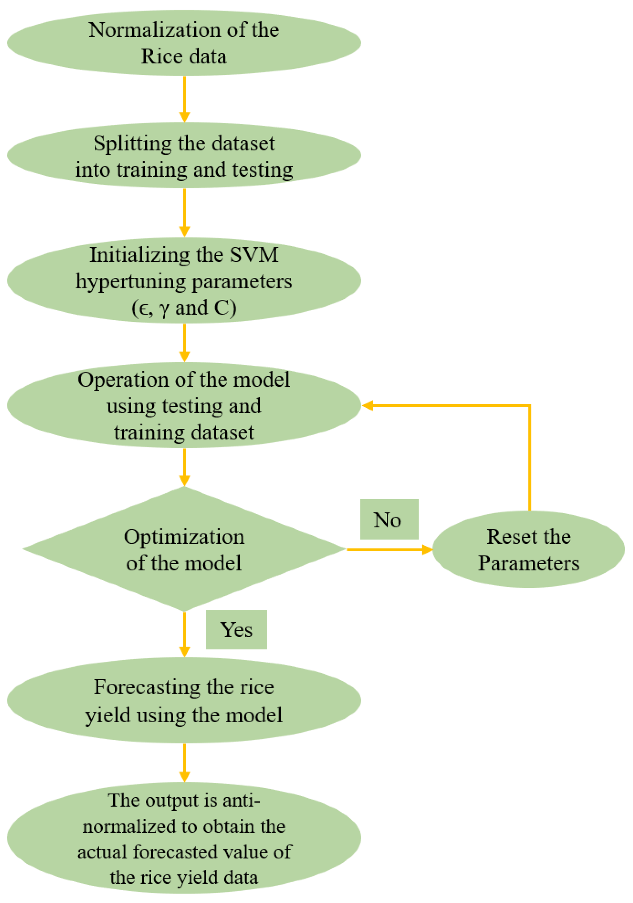
  • The non-linear SVR is used in the study to forecast rice yield data. The kernel function is applied to each data set in order to map the nonlinear observations into a higher-dimensional space where they can be separated. The SVR’s efficiency is determined by the hypertuning parameters, which are interdependent [19,20,21,22]

3.2.3. Schematic Diagram of Performing SVR

Figure 1 presents the process of our SVR methodology.

3.3. Cross-Validation Method

The training set is divided into k distinct subsets using k-fold cross validation. Then, during the entire training process, each subset is used for training and the others k-1 are used for validation. This is done to improve the classification and regression tasks’ preparation. The parameter calibration was performed using the training dataset during the training stage, and the trained model was then evaluated by evaluating the testing results using the RMSE and Mean Absolute Error (MAE) metrics. In this analysis, the average values of RMSE and MAE of 10-folds were used for training results.
The RMSE is the measure of the differences between values predicted by a model or an estimator and the values observed. It can be expressed as
R M S E = 1 N i = 1 N ( y i y ^ ) 2
The MAE is the average of absolute difference between the target and predicted values. It is given as
M A E = 1 N i = 1 N | y i y ^ |

4. Results and Discussion

4.1. Summary Statistics of Rice Parameters

Descriptive statistics such as mean, Standard Deviation (SD), skewness, and kurtosis are evaluated for the Yield (Kg/hectare), Area (Thousand hectares), and Production (Thousand tonnes) for Overall India and major states.
Table 1 summarizes the yield for India as a whole and the top five states. The mean values of West Bengal (1876.755 ± 629.6552), Tamil Nadu (2477.355 ± 734.8786), and Punjab (2991.355 ± 923.6729) are more than average of overall India with their standard deviations. The distribution of rice yield for overall India, Tamil Nadu, and West Bengal exhibiting a positively skewed (0.115, 0.033, and 0.107) and platykurtic curve (−1.235, −1.022, and −1.521) as there is a slight drop of yield seen in recent years. For Bihar, there is a positive skewness (1.215) and leptokurtic (1.243) distribution recorded, as a consistent growth of yield is observed in subsequent years. Similarly, for Punjab and Uttar Pradesh, a negative skewed (−0.84 and −0.217) and platykurtic (−0.345 and −1.443) distribution is found, which implies that yield is declining due the influence of many parameters under consideration.
Table 2 shows the summary statistics of rice crop area under cultivation from 1962 to 2018 for India as a whole and the big five rice-producing states. From the table, the mean and SD values of WB (5375.904 ± 432.7927), UP (5278.316 ± 572.2343), and Bihar (4576.484 ± 897.5415) are allocating major land for rice cultivation and least is observed in Punjab (1739.461 ± 945.8439) and Tamil Nadu (2198.316 ± 386.5147). The skewness and kurtosis values are negatively distributed and follow a platykurtic distribution, which implies that there is a drastic decline in areas under cultivation of the major states and overall India.
Table 3 describes the summary statistics of production of rice for the overall India and major producing states. The mean and SD values of Bihar (5179.959 ± 1378.052), Punjab (5999.959 ± 4040.386), Tamil Nadu (5301.673 ± 1346.065), Uttar Pradesh (8332.887 ± 3942.218), and West Bengal (10268.23 ± 3896.285). Table 3 shows that India and Bihar have positively skewed production and a slight increase, while Punjab, Tamil Nadu, Uttar Pradesh, and West Bengal have negatively skewed production. The kurtosis values for India as a whole are negative, and the major states have a platykurtic distribution. It implies a decline in rice production in the states for the observed years because, as the population grows, the region and production of the states contribute less to the yield earned.

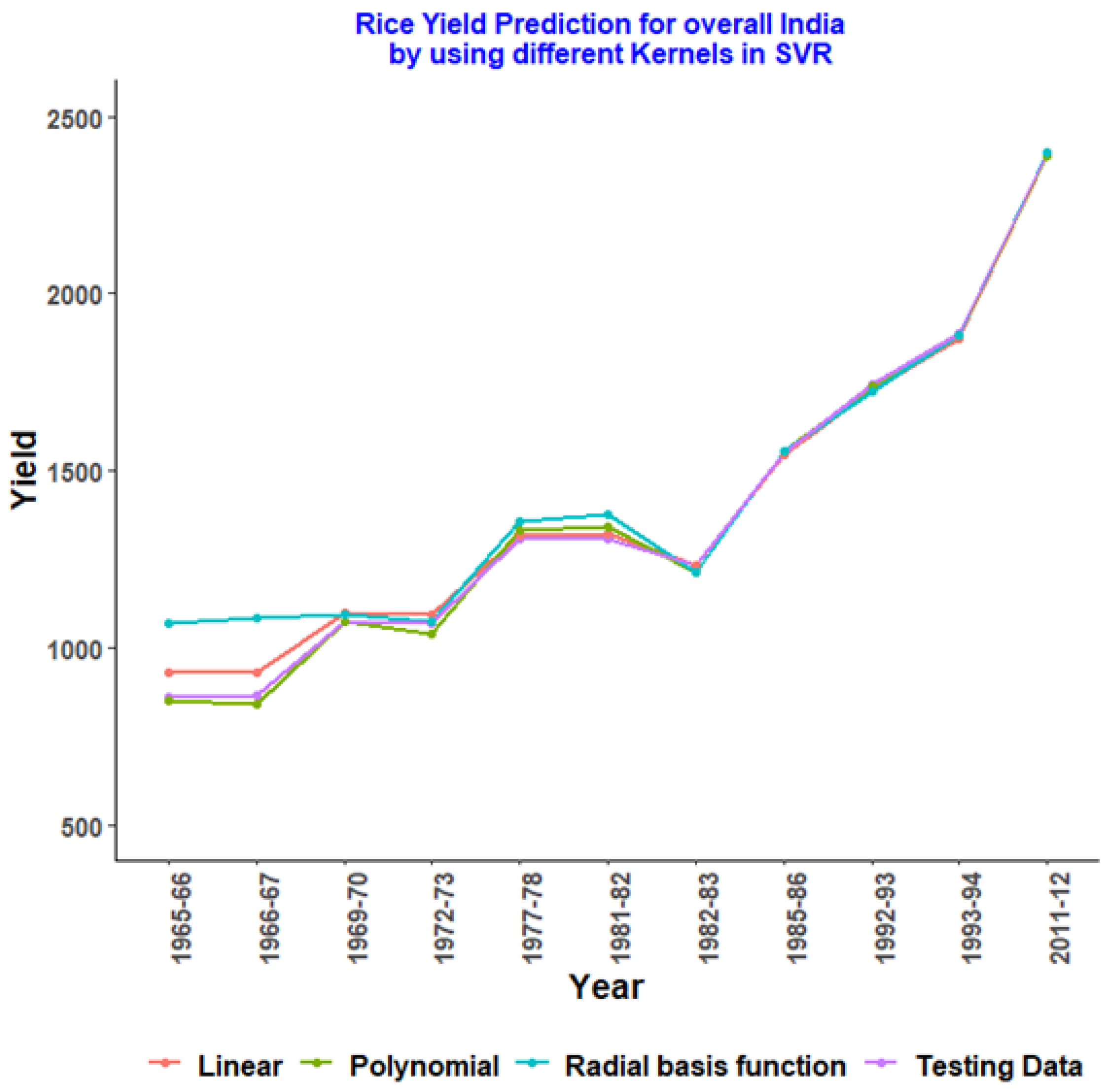
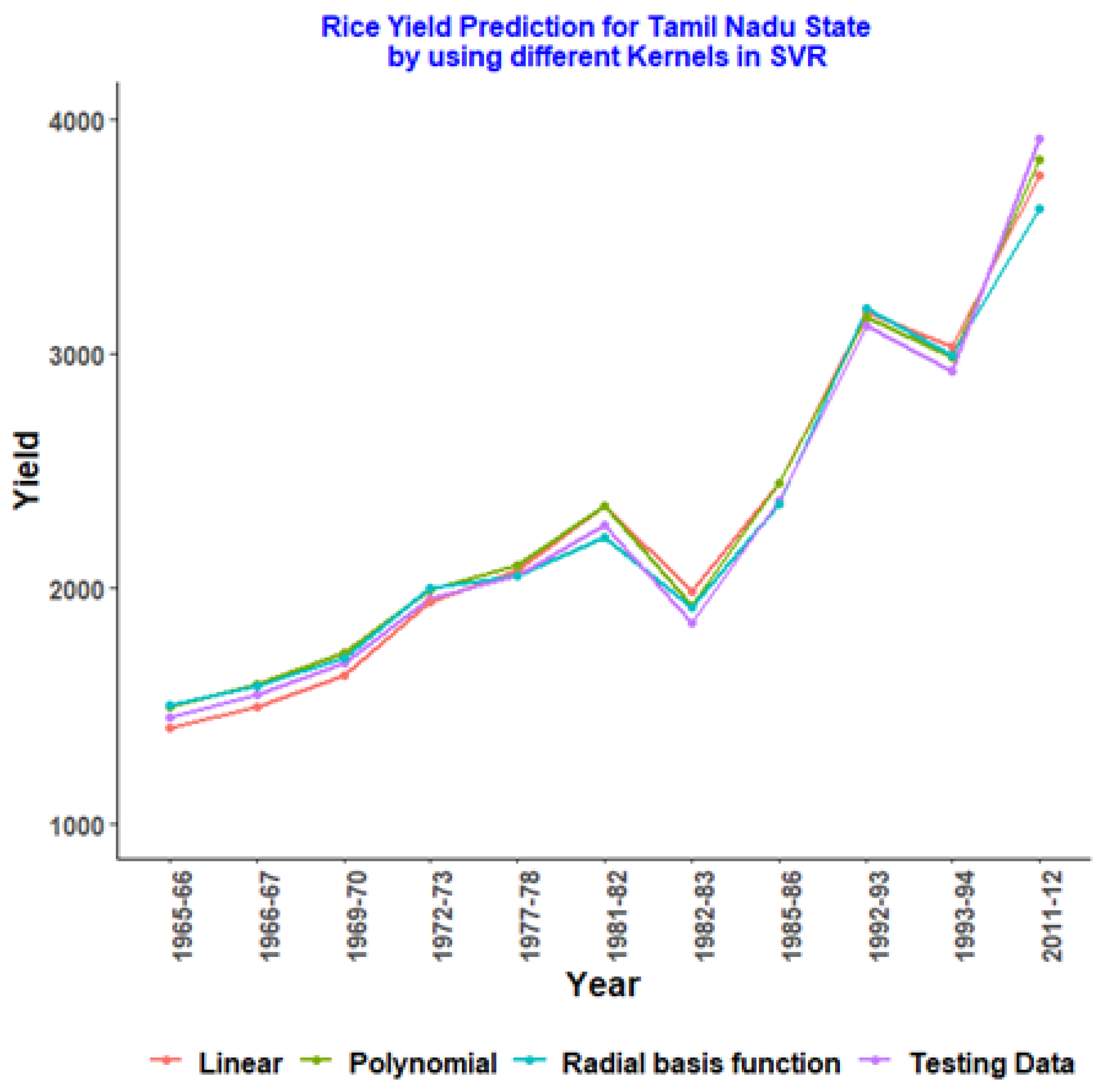
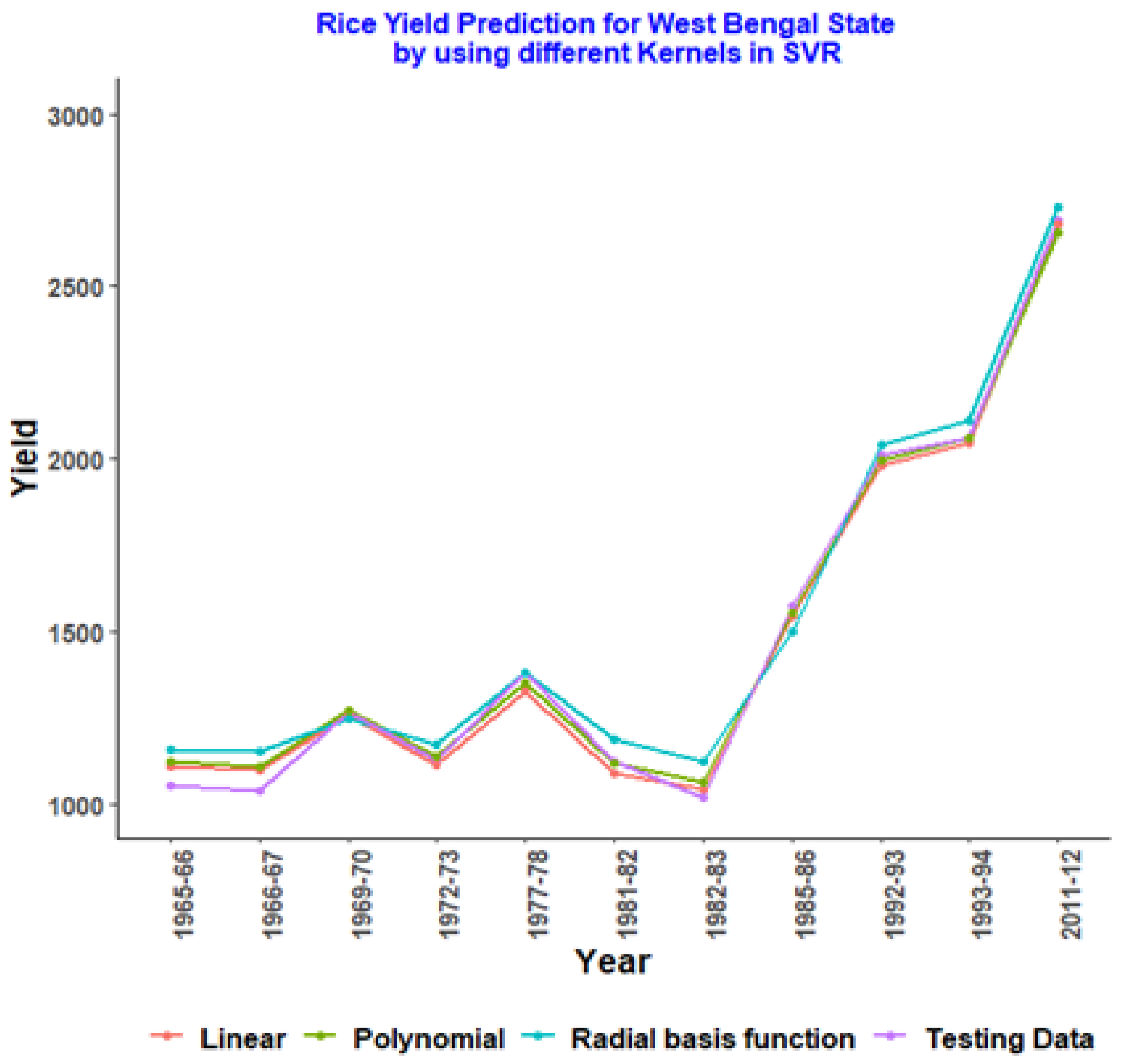
4.2. Rice Yield Prediction of Overall India and Major Producing States Using Various Kernels of SVR with Hypertuning Parameters

Rice yield is primarily affected by the region under cultivation and development, so it was treated as a dependent variable in this analysis, with the other two variables serving as predictors. The best fitted kernels for yield of the overall India and other five states are investigated for both the training and testing data with more accuracy for implementing different user-defined hypertuning parameters such as C, ε , γ, and d. A grid search optimization and k-fold cross validation methods are employed to optimize the hyperparameters. In this study, we consider cross validation (k = 10) to evaluate the model performance of training data of rice yield prediction and to reduce error estimates with less bias and variance in the dataset. The set of hyperparameters (C, γ , and d) is initialized in the given range C (0.05, 1.1), γ (0.05, 0.5) for the polynomial kernel, γ (0.25, 3) for the RBF kernel, d (1, 5) and ε values are set to 0.1 by default. The research focuses on regression models that use SVR and various kernels such as linear, polynomial, and radial basis functions. The findings are summarized in Table 4, Table 5 and Table 6.
Table 4 represents the SVR Linear kernel for overall India and other five states with RMSE, MAE, and predefined cost function.
It is clearly observed that SVR Linear has the best predicted output for the overall India (training and testing datasets) with errors validation such as RMSE (27.52 and 31.056) and MAE (23.0518 and 22.7289) with cost function C = 1.1. For the testing set West Bengal, the SVR Linear kernel has the best predicted output with RMSE and MAE as 31.05 and 27.72, respectively, and with C = 1.05.
Table 5 depicts the optimal values of the parameters of error analysis (RMSE and MAE), degree of polynomial, cost, and γ values using SVR polynomial kernel. SVR Polynomial is the best predicted output for the five major states, i.e., Bihar, Punjab, Tamil Nadu, Uttar Pradesh, and West Bengal in the training dataset by allocating predefined parameters such as degree of polynomial (d (1, 5)), Cost (C (0.05, 1.1)), and scale parameter ( γ (0.05,0.5)). Similarly, for the testing set, Bihar, Punjab, Tamil Nadu, and Uttar Pradesh have SVR Polynomial as the best kernel.
Table 6 depicts the error validation, Sigma ( γ ( 0.25 , 3 ) and cost (C (0.05, 1.1) values of the SVR Radial Basis Function on rice yield of overall India and major states. The results revealed that there is no significant performance for the overall India and the major five states by implementing the SVR RBF kernel.

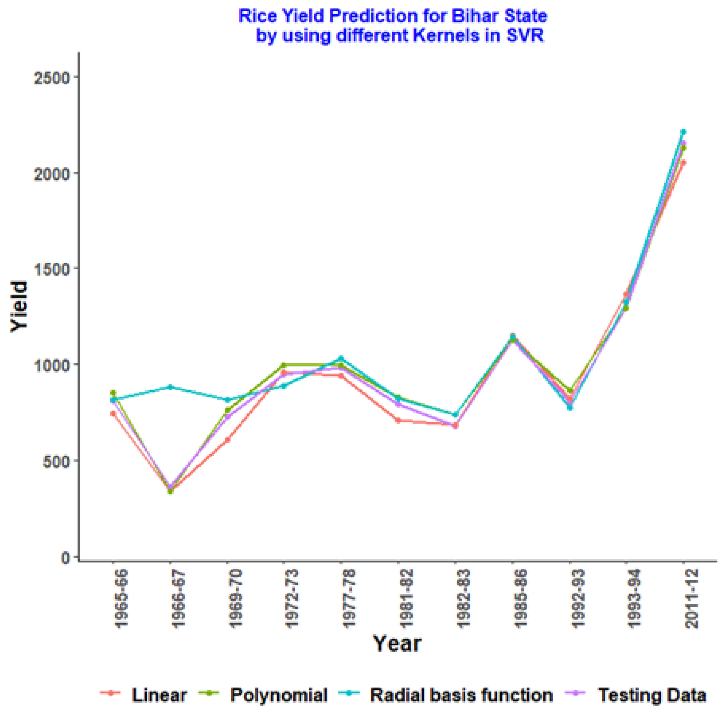
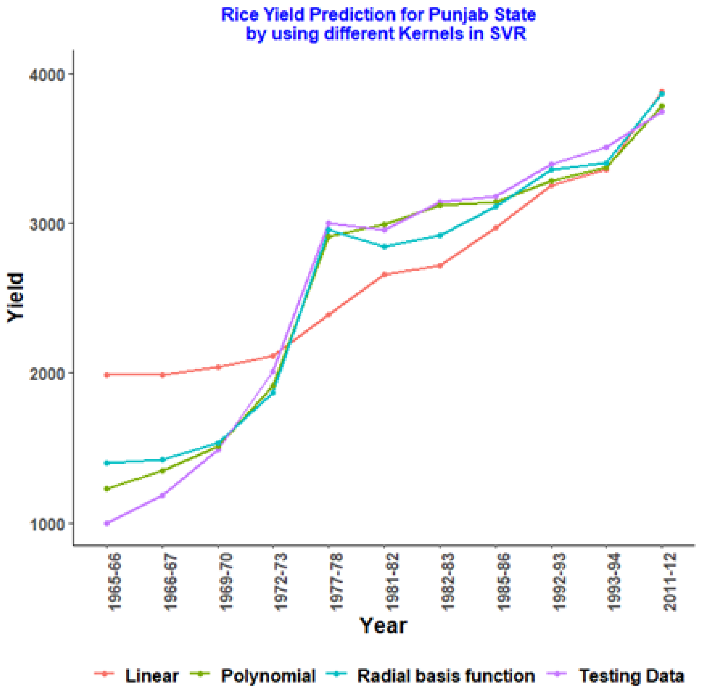
4.3. SVR with Different Kernels for Randomly Allocated Testing Data of Rice Yield

Table 7, Table 8, Table 9, Table 10, Table 11 and Table 12 show the randomly assigned testing data modeled with best fitted SVR kernels such as linear, polynomial, and radial basis function of rice yield training data for India as a whole and the major five rice producing states, as well as graphical representations of the same.
The tables (Table 7, Table 8, Table 9, Table 10, Table 11 and Table 12) and graphical representations (Figure 2, Figure 3, Figure 4, Figure 5, Figure 6 and Figure 7) depict the prediction of testing data (randomly chosen years) of rice yield of the overall India and the major states through various SVR kernels. From the overall summary of Table 13, it is observed that SVR Linear and SVR Polynomial kernels are the best models to predict the rice yield of overall India, and major states show a lower RMSE and MAE as compared to SVR RBF .
When compared to advanced machine learning techniques, traditional methods for forecasting time series data, such as Autoregressive Integrated Moving Average (ARIMA) models, regression models, and other statistical models [23,24,25], which applied to agricultural production, did not yield good approximation values [4,6,7,8,11,12,17,26,27,28]. One of the drawbacks of conventional approaches is that the time series data must be in chronological order when fitting the models, which can be solved by advanced machine learning techniques that select data points at random and suit well–trained models. In comparison to traditional statistical models, the assumptions of non-parametric techniques like SVR were much more versatile in dealing with such non-linear uncertainty situations in order to train the history of rice productivity more accurately. The exploration of various kernels of SVR for major rice-producing states and India as a whole was described in a much better way in this study, allowing for a much better understanding of the exact patterns of rice yield. Even though the major rice-producing states have non-linear (polynomial) patterns, India’s yield has linear patterns.
Graphical representations of SVR kernels with testing data:

5. Conclusions

The demand for rice in India will continue to rise in the coming decades as the country’s population grows. Predicting agricultural production with advanced machine learning techniques is the need of the hour to deliver high reliability and stability prediction performance, which will help India address food security issues and public health concerns. In place of conventional approaches, the models derived from the SVR with different kernels in this study are very useful in handling both linear and non-linear situations of rice production. As a result, the SVR appears to be a viable alternative to other predictive models. Rice yield is limited in this study since it only considers two influencing factors: Area under cultivation and production; however, it can be expanded by adding other influencing factors such as environmental, climatic, and irrigation, fertilizers, and soil fertility parameters to obtain more accurate results. Farmers and crop planners may use these outbreaking results to predict total yields ahead of time and benefit from land allocation and development of various rice crops. This study will provide researchers and policymakers with information to help them concentrate on developing more accurate prediction models to assist the government in implementing new agricultural policies that favor farmers and agribusiness industries.

Author Contributions

K.K.P., C.C., B.M.N., K.R.K., K.P. and C.K. have contributed equally to this work. All authors have read and agreed to the published version of the manuscript.

Funding

This research received no external funding.

Institutional Review Board Statement

Not applicable.

Informed Consent Statement

Not Applicable.

Data Availability Statement

Not Applicable.

Acknowledgments

We would like to express our gratitude to the referees for their positive comments on the manuscript, which have greatly improved it.

Conflicts of Interest

The authors declare no conflict of interest.

References

  1. Kubo, M.; Purevdorj, M. The future of rice production and consumption. J. Food Distrib. Res. 2004, 35, 128–142. [Google Scholar]
  2. Ramesh, D.; Vardhan, B.V. Analysis of crop yield prediction using data mining techniques. Int. J. Res. Eng. Technol. 2015, 4, 47–473. [Google Scholar]
  3. Nishant, P.S.; Venkat, P.S.; Avinash, B.L.; Jabber, B. Crop Yield Prediction based on Indian Agriculture using Machine Learning. In Proceedings of the 2020 International Conference for Emerging Technology (INCET), Belgaum, India, 5–7 June 2020; Institute of Electrical and Electronics Engineers (IEEE): Piscataway, NJ, USA, 2020; pp. 1–4. [Google Scholar]
  4. Jaikla, R.; Auephanwiriyakul, S.; Jintrawet, A. Rice yield prediction using a support vector regression method. In Proceedings of the 2008 5th International Conference on Electrical Engineering/Electronics, Computer, Telecommunications and Information Technology, Krabi, Thailand, 14–17 May 2008; IEEE: Piscataway, NJ, USA, 2008; Volume 1, pp. 29–32. [Google Scholar] [CrossRef]
  5. Medar, R.A.; Rajpurohit, V.S. A survey on data mining techniques for crop yield prediction. Int. J. Adv. Res. Comput. Sci. Manag. Stud. 2014, 2, 59–64. [Google Scholar]
  6. Yousefi, M.; Khoshnevisan, B.; Shamshirband, S.; Motamedi, S.; Nasir, M.H.N.M.; Arif, M.; Ahmad, R. Retracted Article: Support vector regression methodology for prediction of output energy in rice production. Stoch. Environ. Res. Risk Assess. 2015, 29, 2115–2126. [Google Scholar] [CrossRef]
  7. Chen, H.; Wu, W.; Liu, H.-B. Assessing the relative importance of climate variables to rice yield variation using support vector machines. Theor. Appl. Clim. 2016, 126, 105–111. [Google Scholar] [CrossRef]
  8. Su, Y.-X.; Xu, H.; Yan, L.-J. Support vector machine-based open crop model (SBOCM): Case of rice production in China. Saudi J. Biol. Sci. 2017, 24, 537–547. [Google Scholar] [CrossRef] [PubMed]
  9. Govardhan, P.; Korde, R.; Lanjewar, R. Survey on Crop Yield Prediction Using Data Mining Techniques. Int. J. Adv. Comput. Electron. Eng. 2018, 3, 1–6. [Google Scholar]
  10. Oguntunde, P.G.; Lischeid, G.; Dietrich, O. Relationship between rice yield and climate variables in southwest Nigeria using multiple linear regression and support vector machine analysis. Int. J. Biometeorol. 2017, 62, 459–469. [Google Scholar] [CrossRef] [PubMed]
  11. Gandhi, N.; Armstrong, L.J. Rice crop yield forecasting of tropical wet and dry climatic zone of India using data mining techniques. In Proceedings of the 2016 IEEE International Conference on Advances in Computer Applications (ICACA), Coimbatore, India, 24 October 2016; Institute of Electrical and Electronics Engineers (IEEE): Piscataway, NJ, USA, 2016; pp. 357–363. [Google Scholar]
  12. Rahman, M.M.; Haq, N.; Rahman, R.M. Machine learning facilitated rice prediction in Bangla-desh. In Proceedings of the 2014 Annual Global Online Conference on Information and Computer Technology, Louisville, KY, USA, 3–5 December 2014; IEEE: Piscataway, NJ, USA, 2014; pp. 1–4. [Google Scholar]
  13. Kumar, R.; Singh, M.; Kumar, P. Crop Selection Method to maximize crop yield rate using machine learning technique. In Proceedings of the 2015 International Conference on Smart Technologies and Management for Computing, Communication, Controls, Energy and Materials (ICSTM), Chennai, India, 6–8 May 2015; Institute of Electrical and Electronics Engineers (IEEE): Piscataway, NJ, USA, 2015; pp. 138–145. [Google Scholar]
  14. Shakoor, T.; Rahman, K.; Rayta, S.N.; Chakrabarty, A. Agricultural production output prediction using Supervised Machine Learning techniques. In Proceedings of the 2017 1st International Conference on Next Generation Computing Applications (NextComp), Mauritius, 19–21 July 2017; Institute of Electrical and Electronics Engineers (IEEE): Piscataway, NJ, USA, 2017; pp. 182–187. [Google Scholar]
  15. Palanivel, K.; Surianarayanan, C. An Approach for Prediction of Crop Yield Using Machine Learning and Big Data Techniques. Int. J. Comput. Eng. Technol. 2019, 10, 110–118. [Google Scholar] [CrossRef]
  16. Khosla, E.; Dharavath, R.; Priya, R. Crop yield prediction using aggregated rainfall-based modular artificial neural networks and support vector regression. Environ. Dev. Sustain. 2019, 22, 5687–5708. [Google Scholar] [CrossRef]
  17. Alkaff, M.; Khatimi, H.; Puspita, W.; Sari, Y. Modelling and predicting wetland rice production using support vector regression. Telkomnika 2019, 17, 819–825. [Google Scholar] [CrossRef]
  18. Abbas, F.; Afzaal, H.; Farooque, A.A.; Tang, S. Crop Yield Prediction through Proximal Sensing and Machine Learning Algorithms. Agronomy 2020, 10, 1046. [Google Scholar] [CrossRef]
  19. Drucker, H.; Burges, C.J.; Kaufman, L.; Smola, A.J.; Vapnik, V. Support vector regression machines. Adv. Neural Inf. Process. Syst. 1997, 9, 155–161. [Google Scholar]
  20. Gunn, S.R. Support vector machines for classification and regression. ISIS Tech. Rep. 1998, 14, 5–16. [Google Scholar]
  21. Kassambara, A. Machine Learning Essentials: Practical Guide in R; CreateSpace: Scotts Valley, CA, USA, 2017. [Google Scholar]
  22. Lantz, B. Machine Learning with R; Packt Publishing Ltd.: Birmingham, UK, 2013. [Google Scholar]
  23. Mishra, S.; Mishra, D.; Santra, G.H. Applications of Machine Learning Techniques in Agricultural Crop Production: A Review Paper. Indian J. Sci. Technol. 2016, 9, 1–14. [Google Scholar] [CrossRef]
  24. Nagini, S.; Kanth, T.V.R.; Kiranmayee, B.V. Agriculture yield prediction using predictive analytic techniques. In Proceedings of the 2016 2nd International Conference on Contemporary Computing and Informatics (IC3I), Noida, India, 14–17 December 2016; Institute of Electrical and Electronics Engineers (IEEE): Piscataway, NJ, USA, 2016; pp. 783–788. [Google Scholar]
  25. Basso, B.; Liu, L. Seasonal crop yield forecast: Methods, applications, and accuracies. Adv. Agron. 2019, 154, 201–255. [Google Scholar] [CrossRef]
  26. Gandhi, N.; Petkar, O.; Armstrong, L.J. Rice crop yield prediction using artificial neural networks. In Proceedings of the 2016 IEEE Technological Innovations in ICT for Agriculture and Rural Development (TIAR), Chennai, India, 15–16 July 2016; IEEE: Piscataway, NJ, USA, 2016; pp. 105–110. [Google Scholar]
  27. Gandge, Y. A study on various data mining techniques for crop yield prediction. In Proceedings of the 2017 International Conference on Electrical, Electronics, Communication, Computer, and Optimization Techniques (ICEECCOT), Mysuru, India, 15–16 December 2017; Institute of Electrical and Electronics Engineers (IEEE): Piscataway, NJ, USA, 2017; pp. 420–423. [Google Scholar]
  28. Paidipati, K.K.; Banik, A. Forecasting of Rice Cultivation in India–A Comparative Analysis with ARIMA and LSTM-NN Models. ICST Trans. Scalable Inf. Syst. 2020, 7, 1–11. [Google Scholar] [CrossRef]
Figure 1. The process of our support vector regression (SVR) methodology.
Agriengineering 03 00012 g001
Figure 2. SVR kernels for testing data of overall India.
Agriengineering 03 00012 g002
Figure 3. SVR kernels for testing data of Bihar.
Agriengineering 03 00012 g003
Figure 4. SVR kernels for testing data of Punjab.
Agriengineering 03 00012 g004
Figure 5. SVR kernels for testing data of Tamil Nadu.
Agriengineering 03 00012 g005
Figure 6. SVR kernels for testing data of Uttar Pradesh.
Agriengineering 03 00012 g006
Figure 7. SVR kernels for testing data of West Bengal.
Agriengineering 03 00012 g007
Table 1. Summary statistics of yield (Kg/Hectare) for the years 1962–2018.
StatesMeanStandard DeviationSkewnessKurtosis
All India1653.105498.93880.115−1.235
Bihar1187.512458.95051.2151.243
Punjab2991.355923.6729−0.84−0.345
Tamil Nadu2477.671734.87860.033−1.022
Uttar Pradesh1519.801610.1552−0.217−1.443
West Bengal1876.755629.65520.107−1.521
Table 2. Summary statistics of area under cultivation (thousand hectares) for the years 1962–2018.
StatesMeanStandard DeviationSkewnessKurtosis
All India41037.682911.21−0.48−0.945
Bihar4576.484897.5415−0.644−1.33
Punjab1739.461945.8439−0.29−1.464
Tamil Nadu2198.466386.5147−0.033−0.828
Uttar Pradesh5278.316572.2343−0.404−1.18
West Bengal5375.904432.7927−0.336−0.829
Table 3. Summary statistics of production (thousand tonnes) for the years 1962–2018.
StatesMeanStandard DeviationSkewnessKurtosis
All India69143.9324644.120.067−1.316
Bihar5179.9591378.0520.000107−0.005
Punjab5999.5124040.386−0.033−1.384
Tamil Nadu5301.6731346.065−0.128−0.133
Uttar Pradesh8332.8873942.218−0.117−1.453
West Bengal10268.233896.285−0.038−1.659
Table 4. Error analysis and cost values of training and testing datasets by using SVR linear kernel for rice yield prediction.
DatasetStatesRMSEMAECost
TrainAll India27.5205523.051181.1
Bihar80.4091868.361081.1
Punjab297.4711224.22780.25
Tamil Nadu68.6418257.583190.35
Uttar Pradesh43.4731639.075031.1
West Bengal41.0067335.048251.05
TestAll India31.0563222.728861.1
Bihar62.6057450.935861.1
Punjab493.5309401.16930.25
Tamil Nadu84.275672.355830.35
Uttar Pradesh61.4697252.594931.1
West Bengal35.1130130.236461.05
Table 5. Error analysis and degree, cost, and γ values of training and testing datasets by using SVR polynomial kernel for rice yield prediction.
DatasetStatesRMSEMAEDegreeCost γ
TrainAll India28.9792425.07671210.35
Bihar31.260226.966630.50.25
Punjab90.3868774.1052441.10.4
Tamil Nadu49.2795942.1279620.850.25
Uttar Pradesh35.8264329.72098410.25
West Bengal37.913529.8287611.10.4
TestAll India18.2337714.55882210.35
Bihar37.379331.7147630.50.25
Punjab109.316589.2450741.10.4
Tamil Nadu60.8897758.186320.850.25
Uttar Pradesh36.3151131.64557410.25
West Bengal35.7918827.4866911.10.4
Table 6. Error analysis and Sigma ( γ ) and cost values of training and testing datasets by using SVR radial basis function kernel for rice yield prediction.
DatasetStatesRMSEMAESigma ( γ ) Cost
TrainAll India47.9052537.58910.51.1
Bihar65.0970345.877010.251.1
Punjab196.5431150.99222.751.1
Tamil Nadu131.151294.329580.251.1
Uttar Pradesh71.0601653.276360.251.1
West Bengal69.9974958.217590.251
TestAll India94.6094455.986020.51.1
Bihar161.752385.165380.251.1
Punjab174.8837140.02582.751.1
Tamil Nadu102.724567.177550.251.1
Uttar Pradesh98.7009169.968680.251.1
West Bengal69.1217259.528030.251
Table 7. SVR kernels for testing data of overall India.
YearTesting DataLinearPolynomialRadial Basis Function
1965–66862927.3773848.05451067.776
1966–67863928.2253841.44041082.654
1969–7010731099.571074.28191095.163
1972–7310701092.2181040.52721071.356
1977–7813081316.5391331.49161354.699
1981–8213081321.1011342.58611374.131
1982–8312311233.8361214.17361211.379
1985–8615521542.521555.75081556.554
1992–9317441726.4121737.10861725.277
1993–9418881873.5871883.64891883.61
2011–1223932388.3282389.01012399.779
Table 8. SVR kernels for testing data of Bihar.
YearTesting DataLinearPolynomialRadial Basis Function
1965–66812.06749.3555854.4835820.106
1966–67365.93342.1535342.8664880.7237
1969–70729.85612.1557761.4629816.3171
1972–73946.77963.1515995.7426889.5958
1977–78983.18945.5241997.20161029.8179
1981–82793.07711.3524831.4973826.7751
1982–83681.44688.4047738.9844739.2374
1985–861127.611151.0861128.16171142.9612
1992–93806.16823.3341867.6472778.268
1993–941294.781364.0481293.56721325.887
2011–122154.852051.3692125.30522212.6976
Table 9. SVR kernels for testing data of Punjab.
YearTesting DataLinearPolynomialRadial Basis Function
1965–6610001984.9151231.0861400.547
1966–671185.961987.4671344.4061421.784
1969–701490.372040.9761510.0191531.768
1972–732008.412110.8051910.5261869.862
1977–783001.22389.2712913.1052953.451
1981–822956.692653.4542994.6682844.673
1982–833144.052714.2513115.5352918.069
1985–863179.052972.8023140.2173107.372
1992–933390.83251.9273282.863357.642
1993–943507.113359.4783371.5273397.523
2011–123740.953876.6723778.6393864.746
Table 10. SVR kernels for testing data of Tamil Nadu.
YearTesting DataLinearPolynomialRadial Basis Function
1965–661454.211409.091493.5281503.597
1966–671551.081495.7781593.9431586.809
1969–701681.581632.8611728.8351700.689
1972–731953.661941.9071996.3712000.905
1977–782050.462072.6622100.4322052.946
1981–822272.82349.432347.9312216.156
1982–831854.751989.9451925.6941923.1
1985–862371.812449.1832450.1862355.629
1992–933115.593177.1993156.4563190.227
1993–942926.683027.9362984.1512993.174
2011–123917.83757.0443822.6563615.108
Table 11. SVR kernels for testing data of Uttar Pradesh.
YearTesting DataLinearPolynomialRadial Basis Function
1965–66556.72673.1853540.2164763.3959
1966–67452.81566.0447423.2931669.2615
1969–70779.22819.2724799.4894777.9589
1972–73748.22805.2615759.5732778.4787
1977–781068.931049.5311115.01861017.2877
1981–821094.451067.7151157.02511155.563
1982–831114.851088.6141167.61771103.6731
1985–861488.211458.6311533.7731548.5288
1992–931772.771729.7391777.31071820.2415
1993–941902.141841.2171881.80261923.9034
2011–122357.832403.6772319.24432296.3077
Table 12. SVR kernels for testing data of West Bengal.
YearTesting DataLinearPolynomialRadial Basis Function
1965–661051.911108.1851119.5081156.513
1966–671037.771095.9631107.6691152.406
1969–701266.081254.9311271.7391246.331
1972–731127.411114.3211137.8131172.415
1977–781381.571325.8511352.2021377.464
1981–821119.51086.0011114.681184.133
1982–831018.021043.0341062.9541123.664
1985–861573.431545.4161553.5791499.179
1992–932009.91982.7771993.3332039.329
1993–942061.252044.5422058.2192110.904
2011–1226882680.1832657.7772731.098
Table 13. Best fitted regression models with SVR kernels.
StatesDatasetRMSEMAEBest Fitted
SVR Kernels
All IndiaTraining27.5205523.05118Linear
Testing31.0563222.72886
BiharTraining31.260226.9666Polynomial
Testing37.379331.71476
PunjabTraining90.386974.1052Polynomial
Testing109.316589.2451
Tamil NaduTraining49.275642.1280Polynomial
Testing60.889858.1863
Uttar PradeshTraining35.826429.7210Polynomial
Testing36.315131.6456
West BengalTraining37.913529.8288Polynomial
Testing35.1130130.23646Linear
Publisher’s Note: MDPI stays neutral with regard to jurisdictional claims in published maps and institutional affiliations.

