Centralised Smart EV Charging in PV-Powered Parking Lots: A Techno-Economic Analysis

Highlights

Results:

• A centralised smart EV charging algorithm for workplace parking lots is proposed. The algorithm is able to perform cost- or emissions-based EV charging, including a PV system in the optimisation.
• An innovative “benefit-splitting algorithm” is also proposed, to make sure EV owners receive fair compensation for participating in smart charging activities.
• Our results show possible reductions of up to 11% in EV charging costs, 67% in electricity provision costs for the CPO, and 8% in CO₂ emissions if making use of an existing 35 kWp PV system.
• Contracted EV charging capacity for the parking lot can also be reduced, along with EV impact on the power grid.

Implications:

• Centralised smart EV charging is already implementable in public charging with current technology, and it represents a powerful tool to reduce EV charging costs and their impact on power systems and to deliver grid balancing services as well.
• EV owners’ fair compensation should be addressed when designing advanced smart charging algorithms, especially when delivering services where substantial discomfort can be perceived, e.g., Vehicle-to-Grid (V2G).

Abstract

The increased uptake of Electric Vehicles (EVs) requires the installation of charging stations in parking lots, both to facilitate charging while running daily errands and to support EV owners with no access to home charging. Photovoltaic (PV) generation is ideal for powering up EVs, both for environmental reasons and for the benefit it creates for Charging Point Operators (CPOs). In this paper, we propose a centralised V1G Smart Charging (SC) algorithm for EV parking lots, considering real EV charging dynamics, which minimises both the EV charging costs for their owners and the CPO electricity provision costs or the related CO₂ emissions. We also introduce an innovative SC benefit-splitting algorithm that makes sure SC savings are fairly split between EV owners. Eight scenarios are described, considering costs or emissions minimisation, with and without a PV system. The centralised algorithm is benchmarked against a decentralised one, and tested in an exemplary workplace parking lot in Denmark, that includes includes 12 charging stations and one PV system, owned by the same entity. Reductions of up to 11% in EV charging costs, 67% in electricity provision costs for the CPO, and 8% in CO₂ emissions are achieved by making smart use of a 35 kWp rooftop PV system. Additionally, the SC benefit-splitting algorithm successfully ensures that EV owners save money when adopting SC.

1. Introduction

In 2024, 13.6% of new car registrations in the EU were electric (ACEA Auto, New car registrations: +0.8% in 2024; battery-electric 13.6% market share, https://www.acea.auto/pc-registrations/new-car-registrations-0-8-in-2024-battery-electric-13-6-market-share/, accessed on 29 April 2025) a result of a continuous upward trend in the uptake of Electric Vehicles (EVs). The fit-for-55 action plan by the European Commission states that EU countries must reduce their total greenhouse gases emissions by at least 55% by 2030 (compared to 1990 levels) and by 100% by 2050 (Council of the European Union, “Climate Change: What is the EU Doing?”, https://www.consilium.europa.eu/en/policies/climate-change, accessed on 25 April 2025). In order to reach this objective, the transportation sector needs to be decarbonised. Since a large part of the current vehicle fleet features passenger cars, replacing Internal Combustion Engine Vehicles (ICEVs) with EVs is key to reducing CO₂ emissions, since EVs are, at least with the European average electricity mix, significantly less CO₂-intensive than ICEVs [1]. Most EV owners living in densely populated cities rely on public charging opportunities, due to lack of space, but the number of residential EV charging stations in 2024 is still three times higher than the number of public ones worldwide [2]. It is, thus, critical to ramp-up the installation of EV charging stations in different kinds of parking lots. Workplace charging clusters are fairly widespread in modern cities, due to the possibility of charging while at work, sometimes at reduced prices, a benefit that some companies offer to their employees. In order to reduce both CO₂ emissions from EV charging and the related costs, PV systems can be used to power up workplace parking lots, since the production hours match common EV connection times at work. Given that, typically, only one PV system is installed for a group of EV charging stations, a centralised SC algorithm, able to coordinate all the charging stations to effectively exploit the PV production, would be ideal. This would also be beneficial for reducing grid congestion levels, as PV systems can efficiently shave the EV charging peak, and vice-versa [3].

In this article, we firstly propose an easy-to-implement centralised unidirectional (V1G) SC algorithm where all EVs are jointly scheduled, the optimisation constraints facilitate the implementation in a real demonstrator, and the required inputs are minimal (total charged energy of a session, and connection/disconnection time). This makes our solution easily applicable to any parking lot where V1G controllability and basic knowledge of the input parameters (disconnection time, energy target) is available. This information can be provided either by forecasting algorithms or directly by the users via an app [4]. Secondly, we create an innovative SC benefit-splitting algorithm that distributes the SC savings between the EV owners based on the delay they experience in charging their vehicles, ensuring that no-one incurs a loss. We benchmark the performance of our centralised algorithm against a traditional decentralised algorithm, where the optimal charging schedule of each EV is computed independently from the others, regardless of grid constraints (no curtailment). We applied the algorithms to a one-year metered dataset with a resolution of 15 min, which was key to accurately describing the EV charging patterns in the parking lot. The results of this work will be used as a baseline to test the efficiency of the real-life demonstrations planned for the Horizon Europe-funded FLOW Project (FLOW Project, Horizon Europe, https://www.theflowproject.eu/, accessed on 20 April 2025), which focuses on user-centric SC solutions for mass integration of EVs. The remainder of this paper is structured as follows: Section 2 reviews the most relevant scientific literature on the topic of smart EV charging in parking lots, Section 3 introduces the tested optimisation algorithms, while Section 4 describes the analysed case study. Finally, Section 5 shows the main results of the study, and Section 6 draws the main conclusions from the work.

2. Related Work

As shown in

Table 1. Relevant literature overview on smart EV charging techniques for EV charging costs minimisation/PV usage maximisation including a PV system or any equivalent Distributed Energy Resource (DER). Red background means the paper didn’t have the corresponding feature, green background the opposite. Abbreviations: HOR = Hierarchical Optimisation Routine, MPC = Model Predictive Control, RBC = Rule-based Control, LP = Linear Programming, QP = Quadratic Programming, RL = Reinforcement Learning, FLC = Fuzzy-Logic Controller, GA = Genetic Algorithm, MILP = Mixed-Integer Linear Programming, QC = Quadratically Constrained, NLP = Non-Linear Programming, SP = Stochastic Programming, PSO = Particle Swarm Optimisation.

Primary Objective	Methodology	Algorithm Type	Parking Lot	Metered EV Charging Dataset	Charging Continuity Constraint	SC Benefit Split	Refs.
Maximising PV energy usage	HOR	Centralised	YES	YES	NO	NO	[5]
	MPC	Centralised	YES	NO	NO	NO	[6]
	RBC	Centralised	YES	NO	NO	NO	[7]
	PSO	Decentralised	NO	YES	NO	NO	[21]
	SP	Decentralised	NO	YES	NO	NO	[22]
Minimising EV charging costs	LP	Centralised	YES	NO	NO	NO	[8]
	QP	Centralised	NO	YES	NO	NO	[9]
	RL	Decentralised	YES	NO	NO	NO	[10]
	MILP	Decentralised	YES	NO	NO	NO	[23]
	MILP	Centralised	YES	YES	NO	NO	[24]
	GA	Decentralised	NO	YES	NO	NO	[25]
	RT	Decentralised	NO	YES	NO	NO	[11]
	MIQCLP	Centralised	YES	YES	YES	YES	This paper.
Minimising system costs	FLC	Centralised	YES	YES	NO	NO	[26]
	GA	Centralised	YES	NO	NO	NO	[12]
	LP	Centralised	NO	NO	NO	NO	[27]
	LP	Centralised	NO	NO	NO	NO	[28]
	MILP	Centralised	YES	NO	NO	NO	[13]
	MILP	Centralised	YES	NO	NO	NO	[14]
	MILP	Decentralised	NO	YES	NO	NO	[15]
	NLP	Centralised	NO	NO	NO	NO	[16]
	NLP	Centralised	YES	NO	NO	NO	[17]
	PSO	Centralised	NO	NO	NO	NO	[18]
	RBC	Centralised	YES	NO	NO	NO	[29]
Maximising EV charging revenues	NLP	Centralised	YES	NO	NO	NO	[19]
	RBC	Decentralised	NO	YES	NO	NO	[30]
	MILP	Centralised	YES	NO	NO	NO	[31]

, it is possible to approach the problem of EV scheduling in the presence of PV generation from different perspectives, depending on the optimisation objective. A first possibility is aiming to maximise PV energy usage, which, generally, also implies lower system costs (provided the cost for electricity provision is higher than the levelised cost of PV electricity) and lower EV charging costs (if the EV owner receives a discount for charging with PV energy). Existing papers, such as [5,6,7], propose centralised algorithms and analyse the case study of a parking lot. However, only [5] uses a metered EV charging dataset, which is key to realistically describing EV charging behaviour. Another approach is to minimise EV charging costs, usually by giving their owners a discount if they charge when the PV production is able to cover their needs. References [8,9] opted for a centralised algorithm based on linear and quadratic programming, respectively, while the authors in [10,11] chose a decentralised approach based on Reinforcement Learning or rule-based control: two out of these four papers made use of a metered EV charging dataset. Other papers [12,13,14,15,16,17,18] adopt the approach preferred by CPOs, i.e., minimising the system costs. With the exception of [15], they all deploy a centralised approach. Different methodologies are found in this category, from traditional deterministic ones [13,14,15,16,17] to more advanced ones based on genetic algorithms [12] or particle swarm optimisation [18]. In this category, only [15] analyses a metered charging dataset. Another possibility is to maximise the EV charging revenue, taking the perspective of the CPO and opting for a non-linear programming approach, as in [19]. Compared to the reviewed literature, our algorithm was designed with a focus on real-world needs. For example, we included specific constraints, such as “charging continuity”, to avoid EVs going into “sleep” mode, which commonly prevents them from resuming charging [20]. Moreover, our algorithm can be run in real time (e.g., every minute), it is able to adjust the optimal scheduling solution as the parking lot conditions change (e.g., based on the number of connected EVs), and it runs with the minimum required inputs. We also constrain the charging to start immediately, so the owner sees that the EV charging process has started. This also allows us to gage the maximum charging power, which changes based on the battery state of charge and the on-board charger, and which is usually unknown. Further, none of the papers from the literature proposes a way to split the savings from SC between the EV owners. This is particularly relevant when a PV system is used to power up the EVs, due to the higher savings that can be obtained. For example, a group of EVs could be forced to charge at a more expensive time, or to stay longer, due to another group of EVs that require a lot of energy in a shorter time frame. This might limit, or even nullify, the benefit the first group gets from the SC algorithm. Our solution avoids this problem by fairly splitting the SC benefit based on the delay experienced by each user, making sure they are fairly compensated for their “patience”. This is a key element in attracting more EV owners and keeping a stable business model for the CPO. This algorithm is not only valid for workplace charging lots, which often adopt static tariffs, but can be applied also in kerbside charging locations, public parking halls, and others.

3. Methodology

This section describes the EV smart charging problem formulation and the SC benefit-splitting algorithm. The presented methodology works for both the proposed centralised control and the traditional decentralised one. More specifically:

• Decentralised Smart V1G Charging: there is no central coordinator that schedules all EVs at the same time. Each EV is optimised regardless of the others connected at the same time. It is not possible to limit the total charging power of the location to respond to grid limitations; overloading of the parking lot capacity might happen.
• Centralised Smart V1G Charging: a central coordinator schedules all the EVs for optimal costs or emissions whenever an EV connects to or disconnects from the parking lot. It is possible to limit the total charging power of the location to respond to grid limitations.

3.1. Smart EV Charging Problem Formulation

The optimisation problem is formulated as a Mixed-Integer Quadratically Constrained Linear Programming (MIQCLP) problem, with the aim of minimising either the total charging costs for the EV owners and the CPO (i.e., charging when it is cheapest for both) or the equivalent CO₂ emissions (i.e., maximising the consumption when the energy from the grid is coming from renewable sources). The optimisation model, in both the “decentralised” and “centralised” forms, can be formulated as in Equations (1)–(17). Note that, from here onwards, for the sake of brevity, we will omit the “equivalent” term when talking about CO₂ emissions.

Cost-based:

$$\begin{array}{cc}\hfill \underset{\begin{array}{c}{\mathbf{P}}^{\mathbf{EV}};{\mathbf{P}}_{\mathbf{PV}}^{\mathbf{EV}}\\ {\mathbf{P}}_{\mathbf{surp}}^{\mathbf{PV}};\mathbf{Y};\mathbf{T}\end{array}}{min}& \Delta t·\sum _{n=1}^{N\left(t^{*}\right)}\sum _{\tau =1}^{\mathcal{T}}\left(cos{t}_{\tau ,n}^{EV}+cos{t}_{\tau ,n}^{CPO}\right)\hfill \end{array}$$

(1)

Emissions-based:

$$\begin{array}{cc}\hfill \underset{\begin{array}{c}{\mathbf{P}}^{\mathbf{EV}};{\mathbf{P}}_{\mathbf{PV}}^{\mathbf{EV}}\\ {\mathbf{P}}_{\mathbf{surp}}^{\mathbf{PV}};\mathbf{Y};\mathbf{T}\end{array}}{min}& \Delta t·\sum _{n=1}^{N\left(t\right)}\sum _{\tau =1}^{\mathcal{T}}e{m}_{\tau ,n}^{EV}\hfill \end{array}$$

(2)

$$\begin{array}{cc}\hfill \text{with:}& cos{t}_{\tau }^{EV}=P_{\tau ,n}^{EV}·c_{\tau }^{EV}+P_{PV,\tau ,n}^{EV}·c_{PV,\tau }^{EV}\hfill \end{array}$$

(3)

$$\begin{array}{cc}\hfill & cos{t}_{\tau }^{CPO}=P_{\tau ,n}^{EV}·c_{\tau }^{CPO}-P_{PV,\tau ,n}^{EV}·c_{PV,\tau }^{EV}-P_{surp,\tau }^{PV}·c_{\tau }^{spot}·{\displaystyle \frac{1}{N\left(t^{*}\right)}}\hfill \end{array}$$

(4)

$$\begin{array}{cc}\hfill & c_{\tau }^{EV}=\max (c_{min}^{EV},c_{\tau }^{spot}+\Delta c^{CPO})\hfill \end{array}$$

(5)

$$\begin{array}{cc}\hfill & c_{\tau }^{CPO}=c_{\tau }^{spot}+c_{\tau }^{DSO}+c^{TSO}+c^{Tax}\hfill \end{array}$$

(6)

$$\begin{array}{cc}\hfill & e{m}_{\tau }^{EV}=P_{\tau ,n}^{EV}·e{m}_{\tau }^{grid}+P_{PV,\tau ,n}^{EV}·e{m}^{PV}\hfill \end{array}$$

(7)

In this formulation:

• ${\mathbf{P}}^{\mathbf{EV}}$ is the vector of the power absorbed from the power system for each EV and time instant, i.e., $P_{\tau ,n}^{EV}$. ${\mathbf{P}}_{\mathbf{PV}}^{\mathbf{EV}}$ contains the power absorbed directly from the PV system by each EV at every time instant, i.e., $P_{PV,\tau }^{EV}$. Finally, ${\mathbf{P}}_{\mathbf{surp}}^{\mathbf{PV}}$ contains the power injected into the power grid by the CPO-owned PV system.
• The time-dependent cost of charging the EV from the power system is $c_{\tau }^{EV}$, and it constitutes the main revenue for the CPO who owns the EV charging stations; $c_{PV,\tau }^{EV}$ is the cost of charging the EVs from the PV system, which can either be equal to $c_{\tau }^{EV}$ or lower if a discount is applied; $c_{\tau }^{CPO}$ is the time-dependent energy provision cost for the CPO, including all grid tariffs and taxes. Finally, $c_{\tau }^{spot}$ is the cost of electricity in the day ahead (spot) market price, which is the remuneration the CPO receives when injecting power from the PV system into the grid. These values are used to determine the final cost.
• The net tariffs for the DSO and TSO are $c_{\tau }^{DSO}$ and $c^{TSO}$, respectively, out of which the first one is time-dependent only; $c^{Tax}$ is the taxation applied to all the other costs.
• The grams of CO₂ emitted per kWh of energy consumed from the power grid, or from the PV system, are $e{m}_{\tau }^{grid}$ and $e{m}^{PV}$. Note that for the latter, a constant value is assumed.
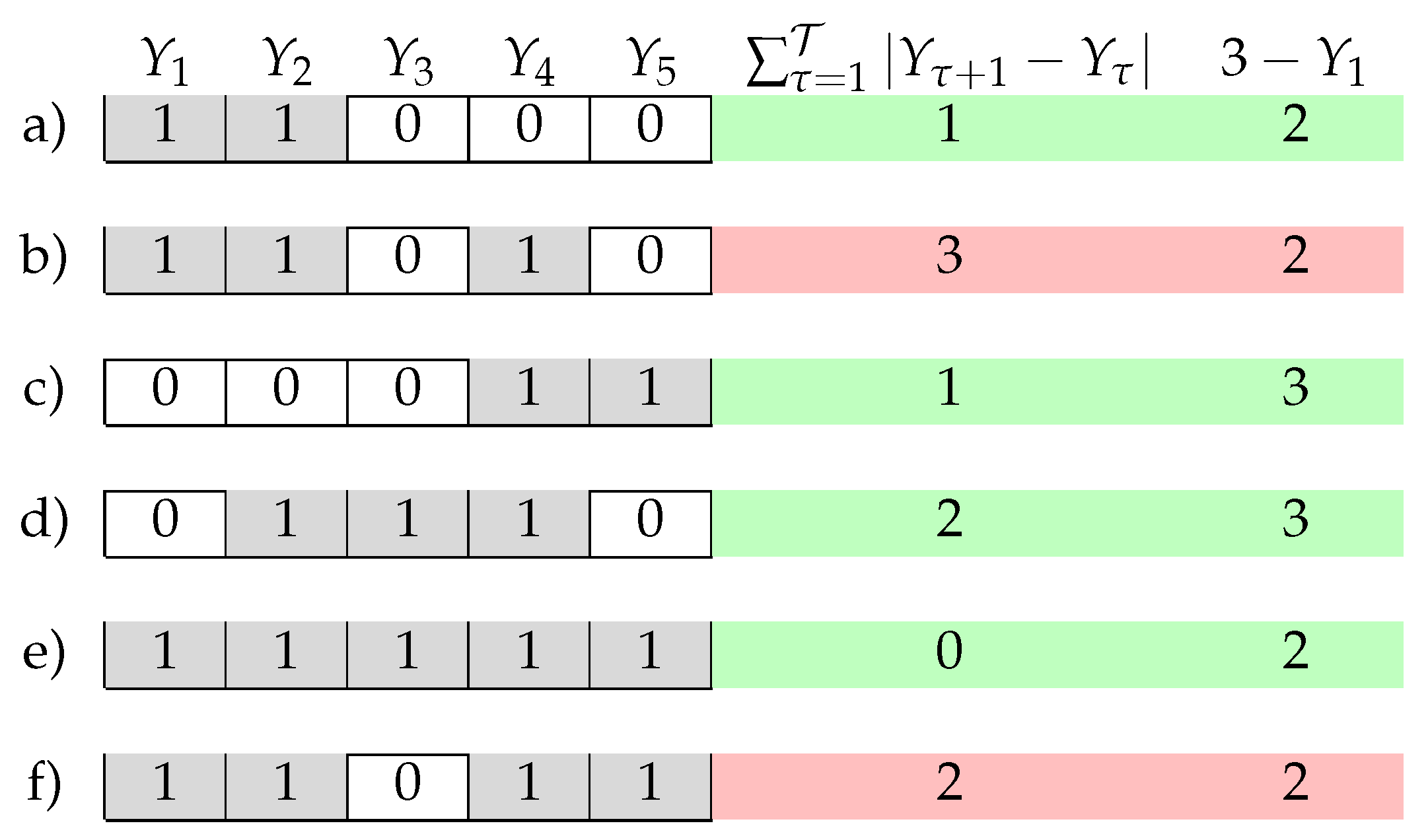
• $\mathbf{Y}$ is the binary variables vector that contains the state of the EVs at each time instant: 0 if the EV is not charging, and 1 if it is.
• $\mathbf{T}$ is the auxiliary variables vector containing the $T_{\tau }=Y_{\tau +1}-Y_{\tau }$ binary variables ranging from −1 to 1 used to linearise the “charging continuity” constraint from Equation (15).
• The time unit along the whole optimisation horizon $\mathcal{T}$ is $\tau$; n is the EV identifier among the number $N\left(t^{*}\right)$ of EVs considered at the $t^{*}$ time the algorithm is run. Note that $N\left(t^{*}\right)=1$ if the decentralised algorithm is considered.
• The simulation timestep in hours is $\Delta t$.

The problem is subject to the following constraints:

$$\begin{array}{cc}\hfill & \Delta t·\sum _{\tau =1}^{\mathcal{T}}\left(P_{\tau ,n}^{EV}+P_{PV,\tau ,n}^{EV}\right)=\Delta E_{n,t^{*}}\hfill \end{array}$$

(8)

$$\begin{array}{cc}\hfill & Y_{\tau ,n}·P_{min}^{EV}\le P_{\tau ,n}^{EV}+P_{PV,\tau ,n}^{EV}\le P_{max,n}^{EV}·Y_{\tau ,n}\hfill \end{array}$$

(9)

$$\begin{array}{cc}\hfill & \sum _{n=1}^{N\left(t\right)}{P}_{\tau ,n}^{EV}\le P_{fuse}\hfill \end{array}$$

(10)

$$\begin{array}{cc}\hfill & 0\le P_{PV,\tau ,n}^{EV}\le P_{\tau }^{PV}·Y_{\tau }\hfill \end{array}$$

(11)

$$\begin{array}{cc}\hfill & P_{\tau ,n}^{EV}\ge 0\hfill \end{array}$$

(12)

$$\begin{array}{cc}\hfill & Y_1=1\hfill \end{array}$$

(13)

$$\begin{array}{cc}\hfill & P_{1,n}^{EV}=P_{max,n}^{EV}\hfill \end{array}$$

(14)

$$\begin{array}{cc}\hfill & \sum _{\tau =1}^{\mathcal{T}}|Y_{\tau +1,n}-Y_{\tau ,n}|=\sum _{\tau =1}^{\mathcal{T}}{T}_{\tau }<3-Y_1\hfill \end{array}$$

(15)

$$\begin{array}{cc}\hfill & Y_{\tau +1,n}-Y_{\tau ,n}\ge -T_{\tau ,n}\hfill \end{array}$$

(16)

$$\begin{array}{cc}\hfill & Y_{\tau +1,n}-Y_{\tau ,n}\le T_{\tau ,n},\hfill \end{array}$$

(17)

where

• $n=1,\dots ,N\left(t\right)$
• $\tau =1,\dots ,\mathcal{T}$.

In the constraints, the following applies:

• The energy request of the n-th EV at the time $t^{*}$ when the algorithm is run is $\Delta E_{n,t^{*}}$, while $P_{max,n}^{EV}$ and $P_{min}^{EV}$ are the maximum and minimum charging power allowed by the on-board charger and charging station.
• $P_{fuse}$ is the maximum power that can be absorbed for the specific parking installation under study, while $P_{\tau }^{PV}$ is the PV production at time $\tau$ (which is null when no PV is considered in the scenario).

In short, Equation (1) signifies that EVs should charge with the objective of minimising both the cost for the EV owners and the provision costs for the CPO. When the objective function is to minimise the CO₂ emissions instead, Equation (2) signifies that EVs should charge when either the energy coming from the grid has a lower carbon content or PV production is available. Equation (8) constrains the energy charged into the battery to the desired value. Equation (9) constrains the total EV charging power between the minimum and maximum levels allowed by the on-board chargers. Similarly, Equation (10) limits the instantaneous aggregated charging power of the EVs to the fuse capacity of the parking lot. Note that PV energy is firstly used to reduce EV consumption; then, it is sold to the grid (due to the higher electricity purchase costs). Equations (11) and (12) imply that both the EV charging power coming from the PV system and the network need to be positive, i.e., no bidirectional charging (V2G) is allowed. Equation (11) also constrains the EV charging power coming from the PV system to be less than the total instantaneous PV production. Equations (13) and (14) force the EV to charge for the first 15 min at maximum power (in a real-time context this would mean no limitations), valuable information for estimating the baseline charging costs without SC (see Section 3.3), and the maximum charging power. Finally, Equations (15)–(17) imply that once the power has started flowing (Y = 1) it cannot stop (Y = 0) and then start again (Y = 1) inside the same session. The mathematical formulation of this constraint is explained in more detail in Appendix A, and it is used to make sure that the EV does not go into “sleep” mode and then cannot be turned on again, which sometimes happens with the models available on the market [20].

3.2. Centralised vs. Decentralised Smart Charging

A few differences exist between the centralised and decentralised charging algorithms, and they require a separate implementation in the algorithm:

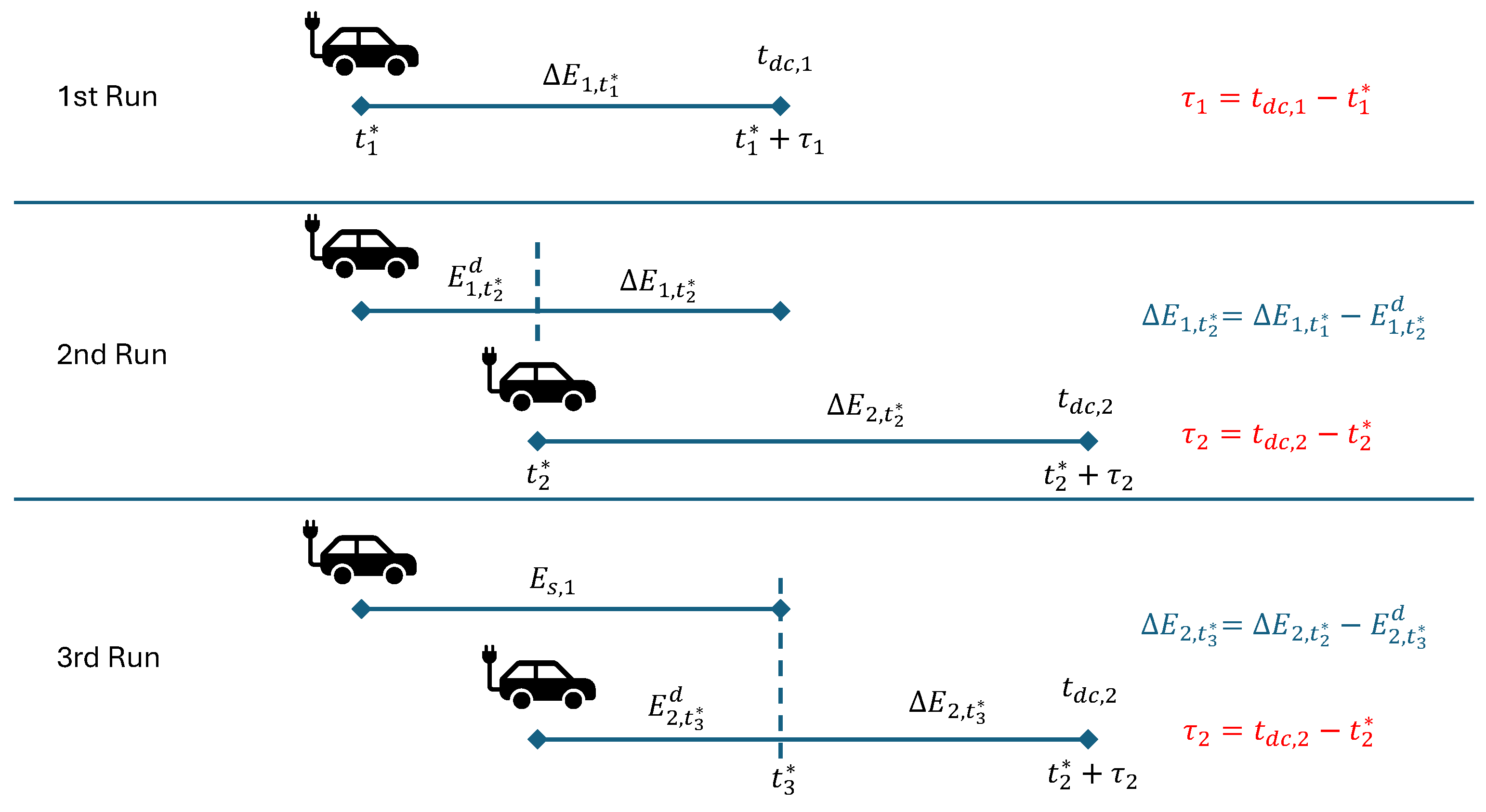
• In the decentralised algorithm, the simulation is separately run for each EV once only; hence, the number of EVs connected at time $t^{*}$ is always equal to one ($N\left(t^{*}\right)=1$). In the centralised algorithm, $N\left(t^{*}\right)$ is the number of EVs connected at the time the optimisation is run, $t^{*}$, which can be any positive integer number up to the number of available outlets.
• In the decentralised algorithm, $\mathcal{T}={\mathcal{T}}_n$ is the number of instants the charging session of the n-th EV lasts. In the centralised one, the formulation changes to Equation (18):

  $$\mathcal{T}=\max \left(\begin{array}{c}{\mathcal{T}}_1\\ {\mathcal{T}}_2\\ ⋮\\ {\mathcal{T}}_{N\left(t^{*}\right)}\end{array}\right)=\max \left(\begin{array}{c}{t}_{dc,1}-t^{*}\\ t_{dc,2}-t^{*}\\ ⋮\\ t_{dc,N\left(t^{*}\right)}-t^{*}\end{array}\right)$$

  (18)

  where $N\left(t^{*}\right)$ is the number of connected EVs at the time $t^{*}$ when the optimisation is run. Here, $t^{*}$ represents one instant in the whole T-long period recorded in the database $t=0,\dots ,T$, while $t_{dc,n}$ is the disconnection time of the n-th EV. In other words, the optimisation horizon is the time between the instant the optimisation is run and the disconnection instant of the EV that stays connected the longest. In this way, the algorithm can be run whenever an EV is disconnected or connected, and at least one optimal schedule is computed for each EV to follow, independently from the success of the algorithm solving the optimisation problem. It can indeed happen that the total parking lot capacity constraint cannot be respected.
• As a consequence of the previous point, while in the decentralised algorithm the optimisation delivers an amount of energy $\Delta E_n=E_n$ that is equal to the total energy request from the n-th EV, in the centralised one the optimiser only charges the fraction of energy $E_n^d$ that has not been charged during the instants before; hence, $\Delta E_n=E_n-E_n^d$.
• Finally, since the centralised algorithm runs every time an EV is connected or disconnected in the parking lot, an additional constraint is needed to keep track of whether the n-th EV was charging in the instant before the current one $t^{*}$, so

  $$Y_{t^{*},n}=Y_{t^{*}-1,n}$$

  (19)

The logic of how the centralised execution works is sketched in Figure 1, where $E_n^d$ is the energy already delivered to the EV at the time the optimisation is run, and where $\Delta E_{n,t^{*}}$ is the energy still to be charged at time $t^{*}$ in the n-th EV. The different communication channels required to realise the SC control are represented in Figure 2. As can be seen in the figure, the EMSP reads the EVSE status (occupied/free) and the maximum EV charging power. Then, the cost of electricity and equivalent CO₂ emissions are estimated based on the information from the TSO and DSO. The instantaneous PV production is also read from the smart meter the PV system is connected to. Once that is done, an EV schedule is estimated and then sent to the EVs.

It is important to note that the power charged in the EVs is not the same as the power absorbed from the grid, as the onboard rectifier is generally considered to have an average efficiency of around 90–95% when operating close to its nominal charging power [32]. The efficiency is not considered in the mathematical formulation because the billing is based on AC measurements. The efficiency should instead be applied when converting into DC power (if V2G was considered, for example).

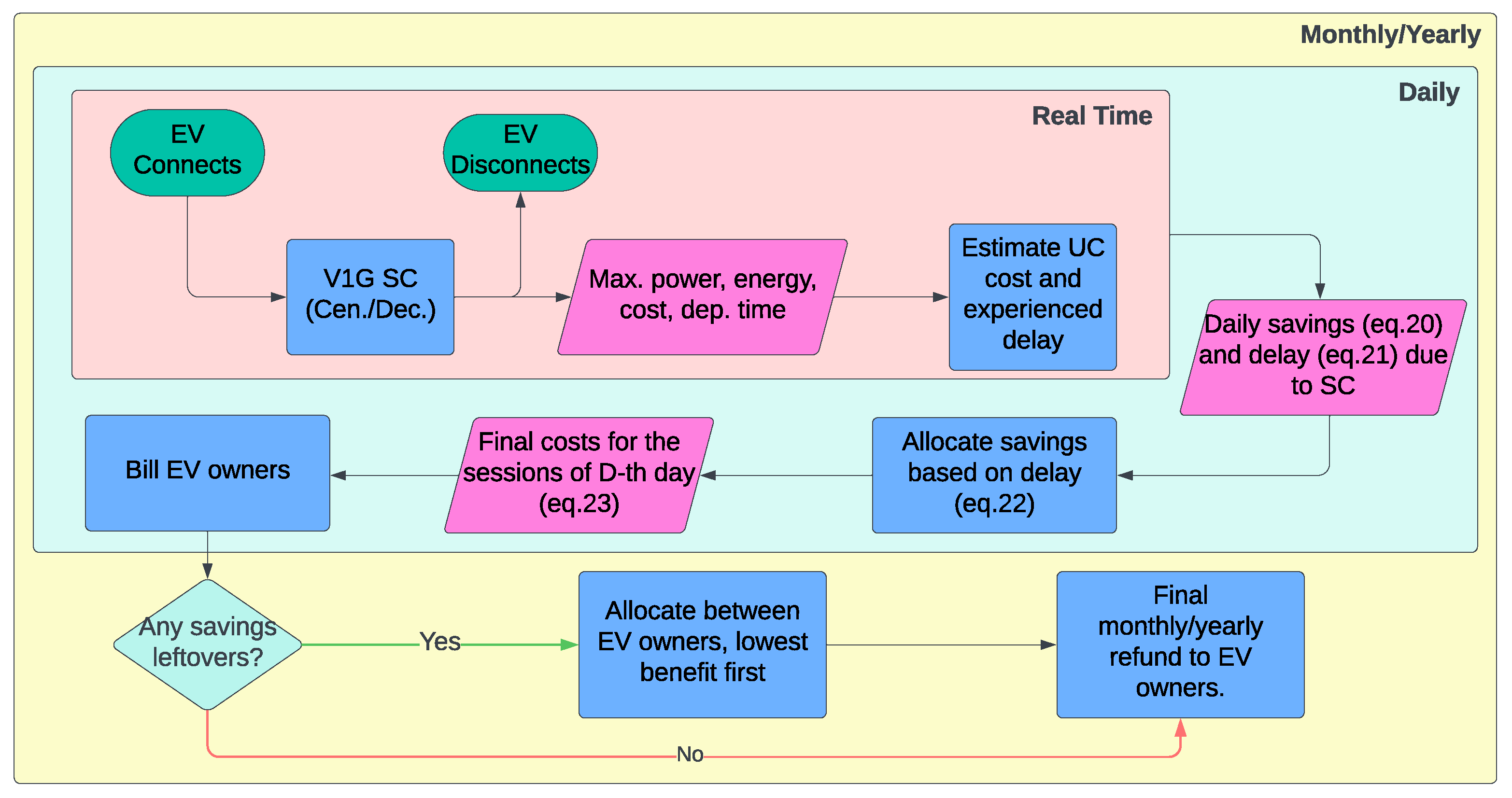
3.3. Benefit-Splitting Algorithm (BSA)

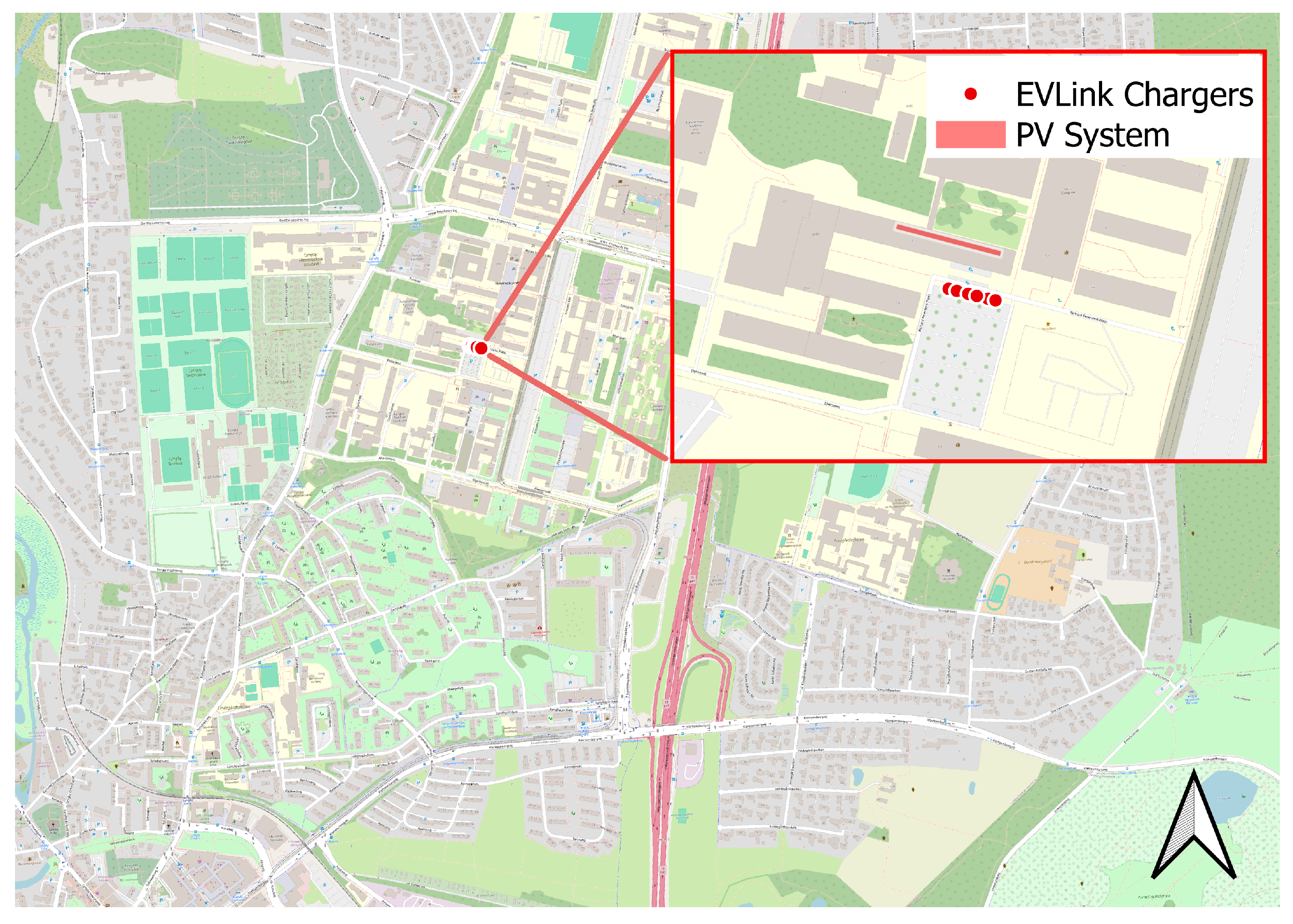
The aim of the centralised SC algorithm is either to minimise the overall electricity expenditures or the CO₂ emissions, usually producing savings in both the electricity provision and EV charging costs compared to the case without SC, here called “Uncontrolled Charging” (UC). These savings need to be split based on their individual contribution to the SC process, making sure every one of them is well-off. In this paper, we propose a two-step benefit-splitting algorithm, whose logic is shown in Figure 3, and which is explained by Equations (20)–(23):

$$\begin{array}{c}cos{t}_n^{EV,UC}=\Delta t·\sum _{t=t_{start,n}}^{t_{end,n}}{P}_{max,n}^{EV}·c_t^{EV}·⌊{\displaystyle \frac{\Delta E_s}{P_{max,n}^{EV}}}⌋\end{array}$$

(20)

$$\begin{array}{c}cos{t}_n^{EV}=\Delta t\sum _{t=t_{start,n}}^{t_{end,n}}{p}_t^{EV}·c_t^{EV}+p_{PV,t}^{EV}·c_{PV,t}^{EV}\end{array}$$

(21)

$$\begin{array}{c}\Delta cos{t}_D=max\left[\sum _{n\mid t_{start,n}\le D·365}\left(cos{t}_n^{UC}-cos{t}_n^{EV}\right);0\right]\end{array}$$

(22)

$$\begin{array}{c}dela{y}_D=\sum _{n\mid t_{start,n}\le D·N_D}\left(t_{end,n}-t_{end,n}^{UC}\right)\end{array}$$

(23)

Note that Equations (20)–(23) use a time index t that represents a $\Delta t$-long instant in the year, with $t=0$ being 00:00 of 01/01 (D = 1) and t = $365·{\displaystyle \frac{1440}{\Delta t}}$ being the last one (D = 365). Since the SC algorithm is run at time $t^{*}$, when a new EV connects to the parking lot, guesses on the session energy $\Delta E_{n,t^{*}}$ and departure time $t_{dc,n}$ are required. In this paper, these values are known beforehand, since we operate under the perfect foresight assumption. The maximum power $P_{max,n}^{EV}$ is recorded, since the first charging instant has no power restriction in Equation (14). Immediately after the charging session ends, the Electro-Mobility Service Provider (EMSP)—which is the company that provides the charging app to the users and bills them for the CPO—estimates a fictitious cost, $cos{t}_n^{UC}$, i.e., the cost that the EV owner would have experienced in UC mode, i.e., without SC. This is achieved via Equation (20), while the delay experienced for the n-th EV is $t_{end,n}-t_{end,n}^{UC}$, i.e., how much longer did it take to reach the required charged energy (at $t_{end,n}$) compared to UC (at $t_{end,n}^{UC}$). The cost with smart charging, $cos{t}_n^{EV}$, is also obtained using the metered power values with Equation (21). At the end of the day, the total daily savings $\Delta cos{t}_D$ and experienced delay $dela{y}_D$ are obtained with Equations (22) and (23) as the sum of the values for the individual EVs. Once the daily savings and delay are obtained for the current day, D, the savings can be split based on the delay experienced by each EV owner. The real money saving, $\Delta$, the final EV charging cost for the ${\widehat{cost}}_n^{EV}$, and the final cost reduction, $\Delta cos{t}_{n,REL}^{EV}$, can thus be mathematically represented as in Equations (24)–(26):

$$\begin{array}{c}\Delta {\widehat{cost}}_n^{EV}=\left\{\begin{array}{cc}min\left(cos{t}_n^{EV,UC};\Delta cos{t}_D·{\displaystyle \frac{t_{end,n}-t_{end,n}^{UC}}{dela{y}_D}}\right)\hfill & \mathrm{if}dela{y}_D>0\hfill \\ 0\hfill & \mathrm{if}dela{y}_D=0\hfill \end{array}\right.\end{array}$$

(24)

$$\begin{array}{c}{\widehat{cost}}_n^{EV}=cos{t}_n^{EV,UC}-\Delta {\widehat{cost}}_n^{EV}\end{array}$$

(25)

$$\begin{array}{c}\Delta cos{t}_{n,REL}^{EV}=100·\left(1-{\displaystyle \frac{{\widehat{cost}}_n^{EV}}{cos{t}_n^{EV,UC}}}\right)\end{array}$$

(26)

Finally, the EMSP proceeds to bill the EV owners by an amount equal to ${\widehat{cost}}_n^{EV}$. On a monthly/yearly basis, if the sum of the daily savings $\sum \Delta cos{t}_D$ along the year is positive then that amount of money is split progressively between the EV owners who charged at the parking lot, prioritizing the ones that had the lowest savings. This can be done by the EMSP as a one-off refund via their application, for example.

4. Case Study

In this section, the case study will be presented. This includes the selected charging cluster and PV system features, the historical EV charging data and tariff structure, and the CO₂ emissions from the Danish electricity system.

The considered parking lot is located in front of Building 325 of the Technical University of Denmark’s (DTU) Lyngby Campus, as shown in Figure 4.

The charging cluster consists of six Schneider Electric EVLink stations, each referred to as an EVSE (Electric Vehicle Supply Equipment) in the following, with two outlets each. The parking lot and the EVSEs are owned by the DTU’s Campus Service (the CPO) and managed by Spirii (the EMSP). Each station is equipped with circuit breakers for overcurrent protection; hence, the maximum power is 22 kW per station or 13.8 kW per outlet. Moreover, the parking lot has a nominal breaker/fuse capacity limit of 68.3 kW (99 A, 3-phase, assuming a constant 230 V L–N voltage), which is set by the CPO, due to the purchased grid capacity. Since the installed parking fuse can withstand up to 113% of the nominal power [33], the maximum power at the parking lot corresponds to 77.2 kW (111.9 A, 3 ph). A nearby PV system, also owned by the DTU’s Campus Service, the CPO, is located on the rooftop of one of the university buildings, and it is oriented at around 12° azimuth (SW) and 30° tilt. These values are slightly suboptimal for total energy yield maximisation purposes, since the PV system should be installed with a 45 degrees tilt and 15° azimuth for that purpose. The installed capacity is 35 kWp, which, in the previously mentioned conditions, yields around 1090 kWh/year/kWp. For this analysis, we assumed that both the PV system and the parking lot were under the same metering point, to be able to net production and consumption.

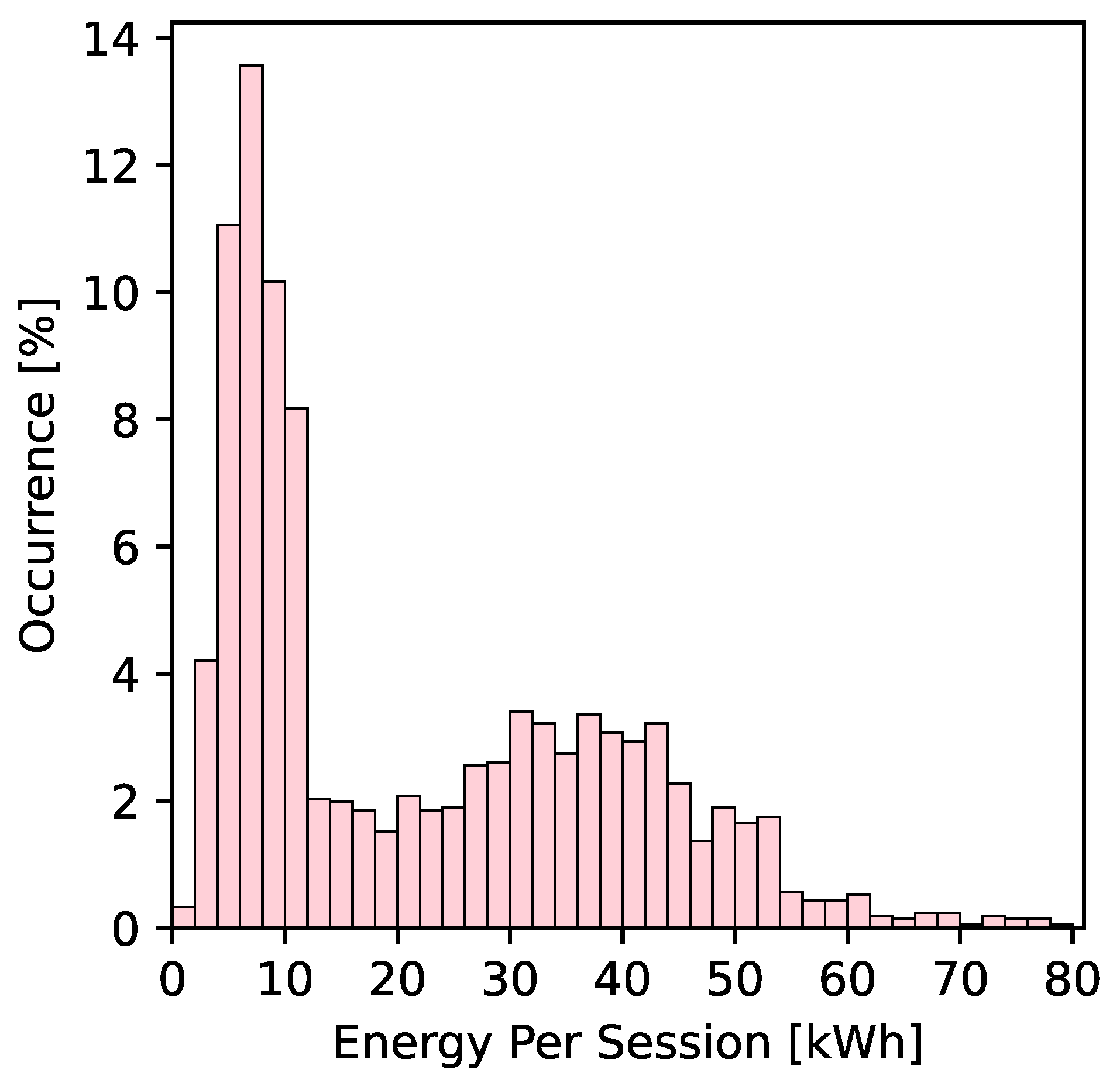
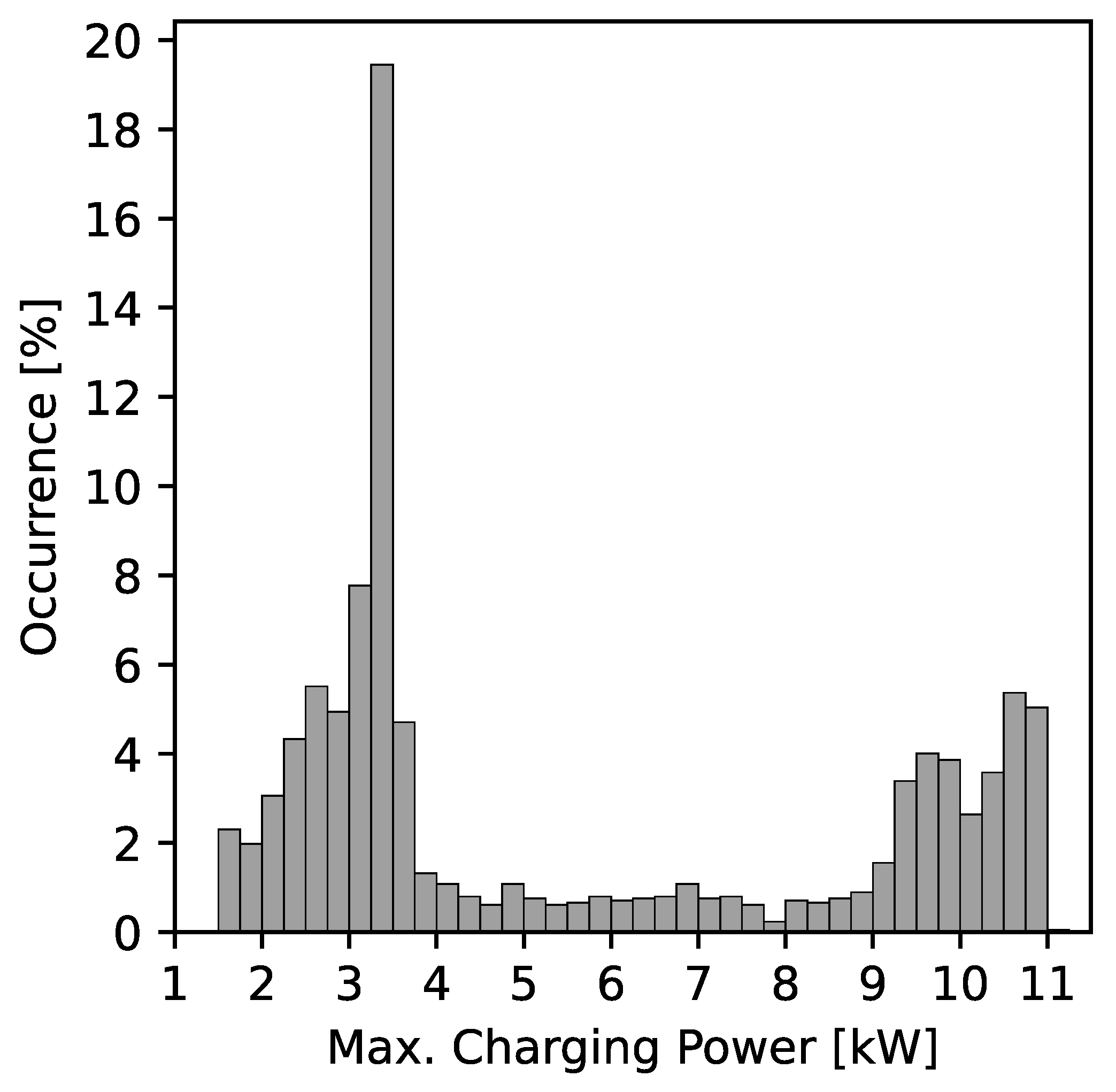
4.1. EV Charging Dataset

The analysed dataset spans one year (2024), and it includes power measurements with 15 min time resolution, as well as the EVSE outlet “state” values. This helped us to identify if the outlet was “free” or occupied by an EV idling or charging. The total number of recorded session was 2124, summing up to 47.1 MWh/year of energy consumption (3.9 MWh/year/outlet). Figure 5 shows the statistical distribution of the energy charged per session, with an evident peak under 10 kWh (50 km driving range, according to online databases (EVdatabase, https://ev-database.org/)) and a secondary peak at 30–40 kWh. Figure 6 shows the statistical distribution of the daily charged energy in the parking lot over the week. The median lowered from 175 kWh/day during weekdays to 25–50 kWh during weekend days. This happened because even though the charging location is public its usage is mostly limited to people working at the nearby DTU campus. The dataset also shows that the usage decreased during summer, as less people were at work due to vacation periods, but this figure is not reported, for the sake of brevity. Figure 7 shows the statistical distribution of the instants when EV owners connected their cars (the charging session almost always “started” immediately), when the power stopped flowing (either the battery was “full” or the EV was disconnected), and, finally, when the EV was disconnected. Finally, Figure 8 shows the statistical distribution of the maximum charging power per session. The EVs were mostly charging at 3.7 kW (16 A, 1 ph), while a few were charging at 11 kW (16 A, 3 ph), which was due to the different market segments that the EV manufacturer targets. All the other intermediate power levels were sessions where the car was almost full, so the EV battery management system limited the maximum power to avoid battery damage.

Figure 7 show that the EV owners mostly connected when they arrived for work, at around 08:00 in the morning, and that their EVs had mostly been charged by around 11:00–12:00 (3–4 h), while disconnections happened when people left, between 15:00 and 17:00. Approximately, the charging process took 3–4 h, with an additional 3–5 h of idling, i.e., connection without charging.

In the UC scenario, i.e., the baseline of our analysis, each EV started charging immediately when connected, and the total energy absorbed by the cluster followed the daily pattern shown in Figure 9.

Each box plot represents the statistical distribution of the power in a particular hour of the day. The cumulative power barely exceeded 65 kW around 09:00, the moment with the highest parking lot occupancy, and the charging sessions were concentrated between 07:00 and 15:00, which are the typical working hours in Denmark. The plot also shows the median charging cost for the EV owners, the electricity provision costs for the CPO, and the median and interquartile range for the CO₂ emissions. It can be noted that the provision costs, which were based on the spot market price, peaked in the early morning and early evening, whereas the emissions were quite stable throughout the day.

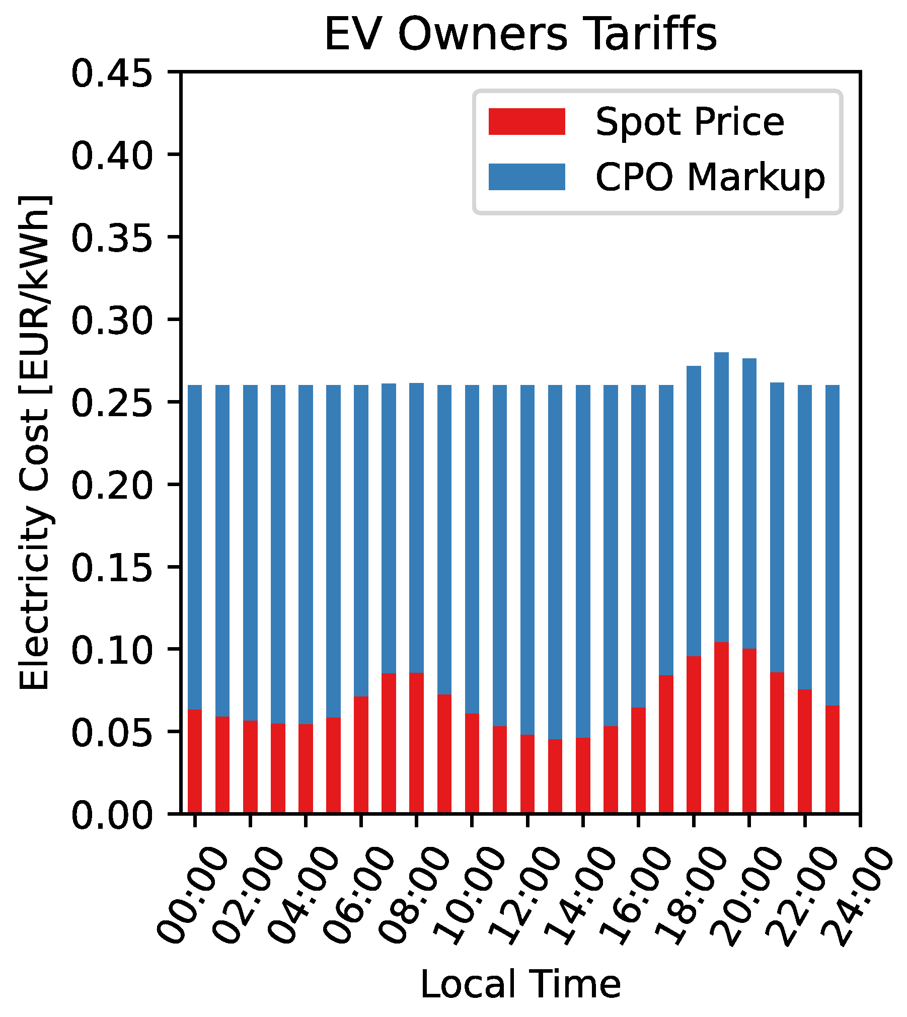
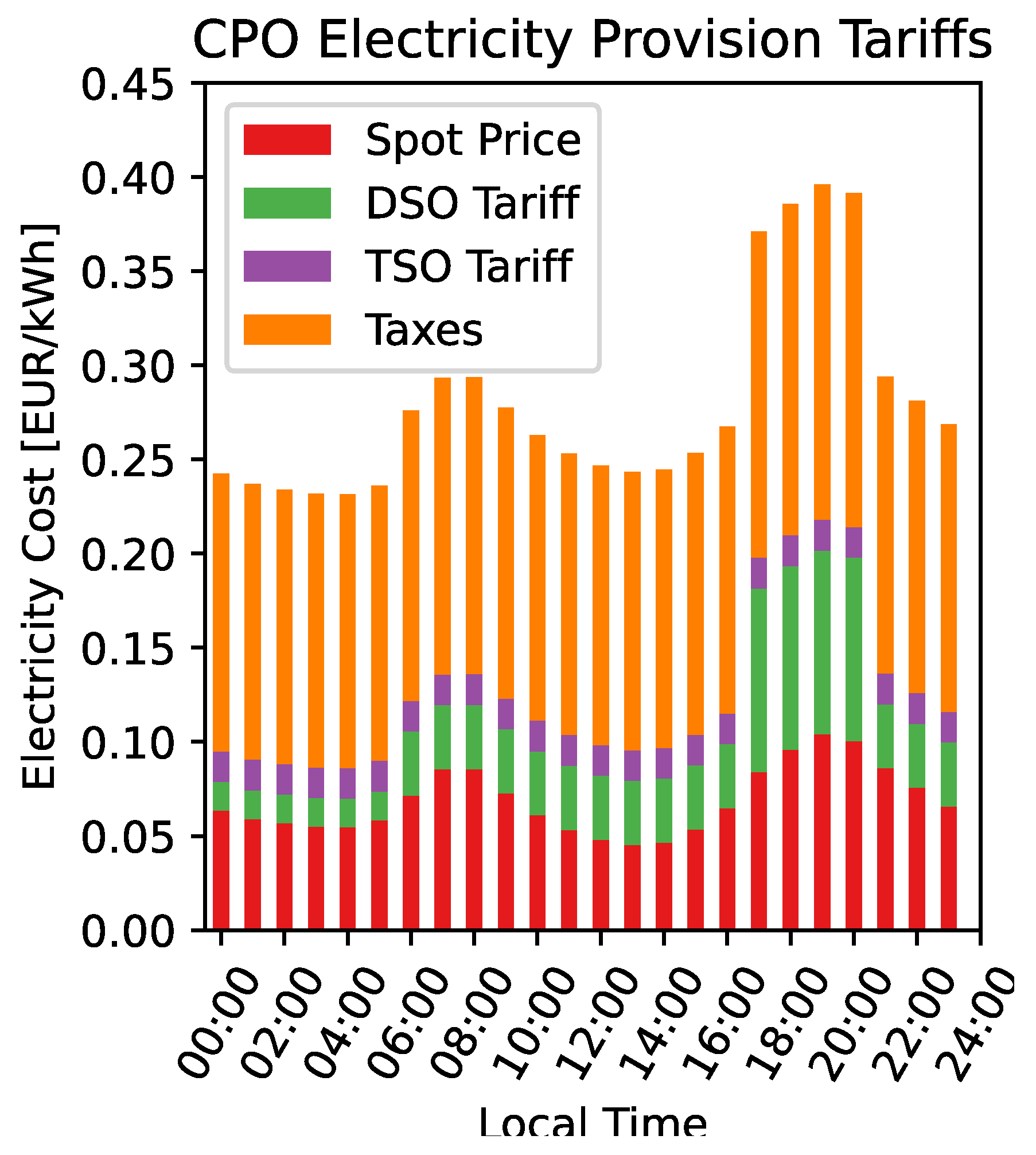
4.2. Costs and Emissions

The dynamic charging cost $c_{\tau }^{EV}$ for the EV owners and the electricity provision costs for the CPO can be obtained analytically as in Equations (5) and (6), and they are represented in Figure 10 and Figure 11, respectively.

For the EV owners, the final charging cost was the combination of the day-ahead market price $c_{\tau }^{spot}$ for the DK2 area (Energinet Database for Spot Prices, https://www.energidataservice.dk/tso-electricity/Elspotprices, accessed on 18 April 2025) and a EUR 0.175/kWh markup fee $\Delta c^{CPO}$ imposed by the CPO, with a lower cap $c_{min}^{EV}$ at EUR 0.26/kWh. For the CPO, instead, other than the spot market price, DSO and TSO tariffs applied, as well as taxes (VAT included). As shown in Figure 10, since the spot market price was quite low, the minimum cap of EUR 0.26/kWh was almost always the final cost, and this helped the EV owners to determine the final cost of the session before starting it. In turn, the CPO had more variable costs, mostly due to the variable DSO tariff $c_{\tau }^{DSO}$, which was added on top of the TSO one $c^{TSO}$ and the VAT $c^{Tax}$. As shown in Figure 11, the hourly average of $c_{\tau }^{CPO}$ was around the EUR 0.26/kWh mark, which means this is currently not a profitable business model for the CPO. This happened for two reasons: (i) the service is mostly intended as a benefit to employees, rather than a profit-generating one; (ii) the markup fee $\Delta c^{CPO}$ had not been updated since the recent change in DSO and TSO tariffs. The value of $c_{PV,\tau }^{EV}$ used in Equations (3) and (4) was assumed to be either EUR 0.087/kWh or 99% of $c_{\tau }^{EV}$. The first value is the LCOE of a PV system in Denmark, EUR 0.085/kWh, obtained considering EUR 1250/kWp of CAPEX (IRENA, Renewable Power Generation Costs in 2022, https://www.irena.org/Publications/2023/Aug/Renewable-Power-Generation-Costs-in-2022, accessed on 21 April 2025) and a 2% operation and maintenance cost per year [34]. The latter value was chosen as being very close to $c_{\tau }^{EV}$—to preserve the incomes of the CPO from the EV charging activities—but still not equal, so as to prioritize PV self-consumption over grid absorption. As far as the additional DSO tariff $c_{\tau }^{DSO}$ was concerned, C-type tariffs applied (Radius net tariff model: https://radiuselnet.dk/elnetkunder/tariffer-og-netabonnement/, accessed on 21 April 2025), since this type of installation (LV-connected, no dedicated substation, maximum power under 110 kW) still falls into the C-type. For the sake of completeness, we repeated the simulation with the B-low type, which is the standard one for public charging places, and the results did not significantly change, so they are not reported. Note that the costs for purchasing and installing the EVSEs are not included, since this paper is not aimed at evaluating the investment payback, but rather at benchmarking the SC algorithm performance.

The carbon dioxide emissions associated with energy production in Denmark, $e{m}_{\tau }^{grid}$, were procured from the website of the Danish TSO (Energinet Database for CO₂ Emissions, https://www.energidataservice.dk/tso-electricity/$CO_2$Emis, accessed on 20 April 2025). In the recorded period, the median CO₂ emissions were around 69 gCO₂/kWh, as shown in Figure 9. Whenever the EV owners consumed energy produced by a PV system, the constant value of 50 gCO₂/kWh (NREL, Life Cycle Greenhouse Gas Emissions From Solar Photovoltaics (2012), https://www.nrel.gov/docs/fy13osti/56487.svg, accessed on 20 April 2025) coming from the life cycle assessment of the emissions for a PV system was considered. Eight scenarios were analysed in total, either minimising the charging/CPO costs or the CO₂ emissions. A summary of the features of each scenario can be found in

Table 2. Overview of the analysed scenario features.

Scenario	S1	S2	S3	S4	S5	S6	S7	S8
Centralised			X	X	X	X	X	X
Decentralised	X	X
Min. Cost	X		X		X	X
Min. CO2		X		X			X	X
PV System					X	X	X	X
PV Discount					X		X

.

Scenarios S1 and S2 were the decentralised ones, aimed at either minimising the EV charging/CPO provision costs or the CO₂ emissions. S3 used the centralised SC algorithm to minimise the charging and provision costs, while S4 minimised the CO₂ emissions. S5 and S6 included the 35 kWp PV system, and they minimised the charging costs with and without a discount for the EV owners who charged from the PV system, respectively. Finally, S7 and S8 considered the same hypotheses as S5 and S6, but with the objective of minimising the CO₂ emissions. In Section 5, the results of the optimisations for these different scenarios are shown.

5. Results

The results of the eight analysed scenarios are shown in

Table 3. Summary of the results for scenarios S1–S8, where negative reductions represent an increase of the value. The different background colors represent the different analysed parameters.

EV Charging Costs
	S1	S2	S3	S4	S5	S6	S7	S8
UC	12.90 k€	12.90 k€	12.90 k€	12.90 k€	10.17 k€	12.86 k€	10.17 k€	12.86 k€
SC	12.76 k€	12.84 k€	12.76 k€	12.83 k€	9.08 k€	12.73 k€	9.90 k€	12.79 k€
Red.	1.10%	0.50%	1.10%	0.50%	10.70%	1.00%	2.70%	0.50%
Equivalent CO2 Emissions
	S1	S2	S3	S4	S5	S6	S7	S8
UC	3.62 t CO2	3.62 t CO2	3.62 t CO2	3.62 t CO2	3.16 t CO2	3.16 t CO2	3.16 t CO2	3.16 t CO2
SC	3.68 t CO2	3.41 t CO2	3.60 t CO2	3.41 t CO2	3.05 CO2	3.05 t CO2	2.92 t CO2	2.92 t CO2
Red.	−1.80%	5.80%	0.40%	5.60%	3.50%	3.50%	7.60%	7.60%
CPO Electricity Provision Costs
	S1	S2	S3	S4	S5	S6	S7	S8
UC	13.24 k€	13.24 k€	13.24 k€	13.24 k€	7.06 k€	4.37 k€	7.06 k€	4.37 k€
SC	12.71 k€	13.14 k€	12.89 k€	13.13 k€	5.09 k€	1.44 k€	6.55 k€	3.65 k€
Red.	4.10%	0.80%	2.70%	0.90%	27.90%	67.10%	7.20%	16.50%

. All the algorithms were implemented and solved with the Gurobipy 12 solver for Python 3.9 on a 12th Gen Intel Core i7-1280P with 20 logical cores and 2 GHz maximum frequency. The centralised algorithm takes longer to solve than the decentralised one, but the solution time is still fast enough to allow for a real-time application of the algorithm. For reference, S6 took a total of 219 s to be solved for a year of data, or about 0.056 s on average per run of the algorithm.

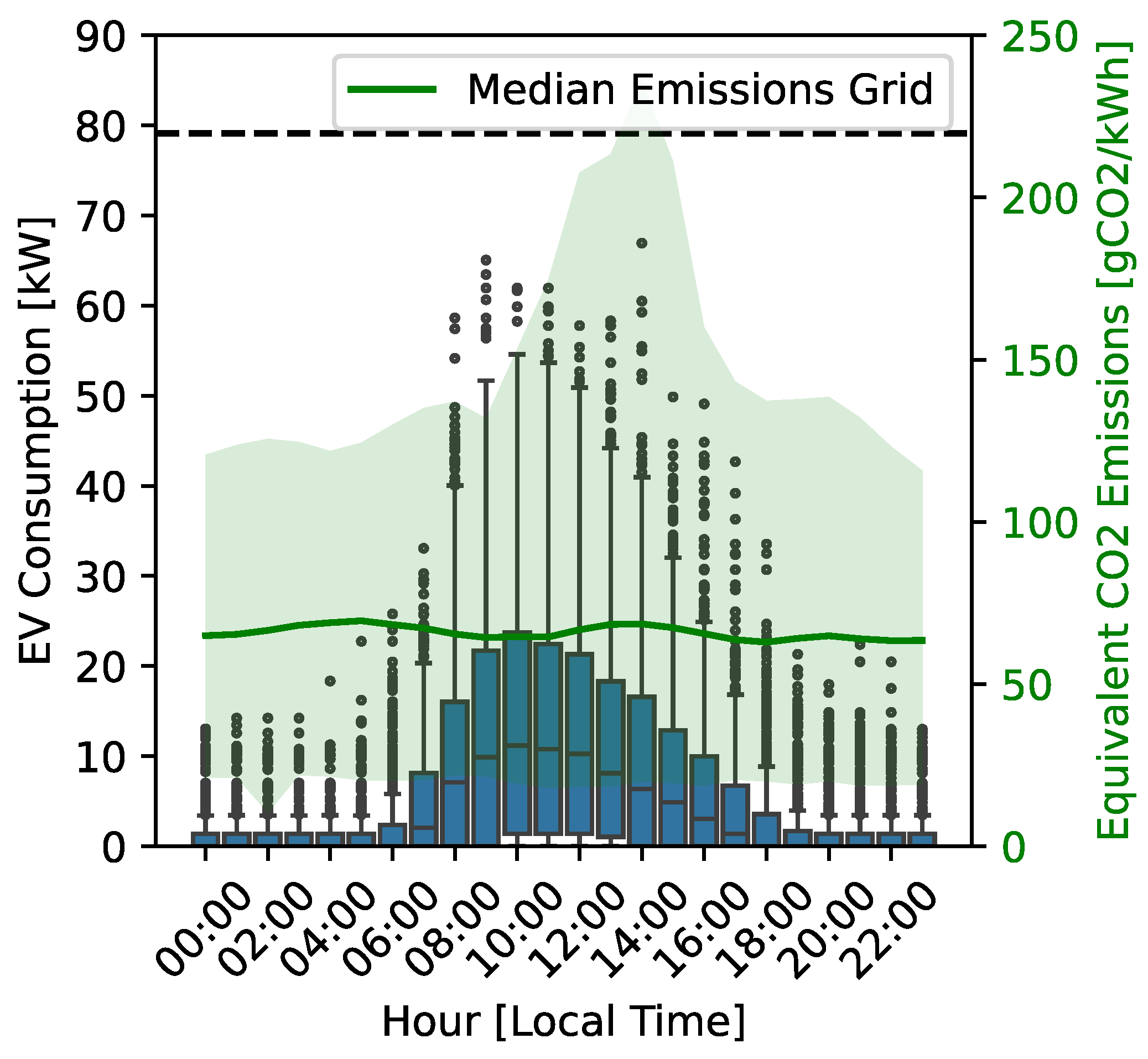
5.1. S1 & S2—Decentralised Optimisation Results

In the cost-based optimisation (S1), we minimised both the EV charging and CPO provision costs. These two prices, as described in Section 4.2, are both based on the spot market price but increase by either the CPO markup fee or the different grid tariffs and taxes. The resulting SC charging patterns are presented in Figure 12 and Figure 13 for S1 and S2, respectively.

For S1, the EV charging was moved to the central hours of the day, as the peak was shifted from 08:00 (as in Figure 9) to 13:00. This shift of 4–5 h allowed the EVs to charge when the CPO cost was lowest, i.e., away from the morning price peak of 08:00–09:00. The maximum recorded power was just over 70 kW; thus, no overloads were detected. Since the electricity cost for the EV owners was flatter than the CPO provision tariff, the SC performed with these conditions favoured the CPO. This can be clearly seen in the results of Table 3, where S1 produced a reduction of 1.1% in EV charging costs, and 4.10% in electricity provision costs for the CPO. Since the EV charging was moved to 13:00—which, as seen in Figure 9, had higher CO₂ emissions per kWh—the total emitted CO₂ increased by 1.8 % (negative reduction). For S2, the resulting charging pattern was smoother, due to the more “stable” values of the CO₂ emissions per kWh throughout the day. As shown in Figure 13, the EVs tried to avoid charging during the hours between 12:00 and 14:00, due to the higher variability of the emission values. The peak charging value was also around 70 kW, so no overload events were noted for S2 either. Table 3 reports a 5.80% reduction in CO₂ emissions and irrelevant costs reductions for both the CPO and EV owners.

5.2. S3 & S4—Centralised Optimisation Results

Scenarios S3 and S4 used the same “external” optimisation signals as S1 and S2, but made use of the centralised SC algorithm to dynamically schedule the EVs whenever a change in parking lot occupancy was detected (i.e., a new EV connected). The related EV charging patterns are presented in Figure 14 and Figure 15 for S3 and S4, respectively.

The charging patterns are clearly very similar to the decentralised ones, since the price and emission signals were the same. The results from Table 3 also show that in S3 the costs reduction for the EV owners was the same as in S1, while the total emissions decreased by 2.2% compared to S1. This was due to the lower peak values recorded in the centralised optimisation algorithm, since some of the charging sessions were moved to a later hour of the day. As a consequence, the CPO provision costs were 1.40% higher in S3 than in S1. In S4, the results were extremely similar to S2.

Sensitivity Analysis on the Fuse Capacity

The current nominal power rating on the cluster fuse was 68.3 kW; hence, approximately 6 out of 12 EVs could be charged at full power (11 kW) at the same time. A lower fuse limit would reduce the number of EVs that could be charged simultaneously, while a higher limit would provide better optimisation results, as more EVs can follow an optimal charging schedule. Higher fuse capacities would, of course, be more expensive to maintain for the CPO. Since we were now using a centralised algorithm, it was possible to reduce the maximum fuse capacity and to test how well the SC algorithm responded, in terms of overloads and charging costs/emissions. The results are showcased in

Table 4. Summary of the costs-based optimisation results from S3 with different fuse capabilities.

Nominal Fuse Limit [kW]	30	40	50	60	70
Fuse Limit [A]	23	31	39	47	55
Fuse Overload	1.4%	0.2%	0.0%	0.0%	0.0%
Energy Demand [MWh]	47.1	47.1	47.1	47.1	47.1
Unserved Energy UC	3.54%	0.54%	0.02%	0.00%	0.00%
Unserved Energy SC	1.77%	0.155%	0.00%	0.00%	0.00%

for a number of fuse capacities in the case of S3.

When the nominal fuse capacity was reduced from 70 kW to 50 kW, the capacity was never saturated. If the fuse capacity was further reduced to 30 kW, the fuse was overloaded by 3.54% and 1.77% of the time for UC and SC, respectively. These considerations led us to conclude that (i) the fuse capacity could be reduced down to 40 kW (31 A) without noticeable issues, with a connection cost reduction for the CPO of EUR 3900 (assuming that EUR 130/A is the current connection cost for the CPO), and (ii) smart charging (and “controllability” in general) is helpful to avoid grid congestion. In the near future, with increased utilisation of public EV charging points, exploiting the grid capacity in the most efficient way will be key to completing the transition to e-mobility.

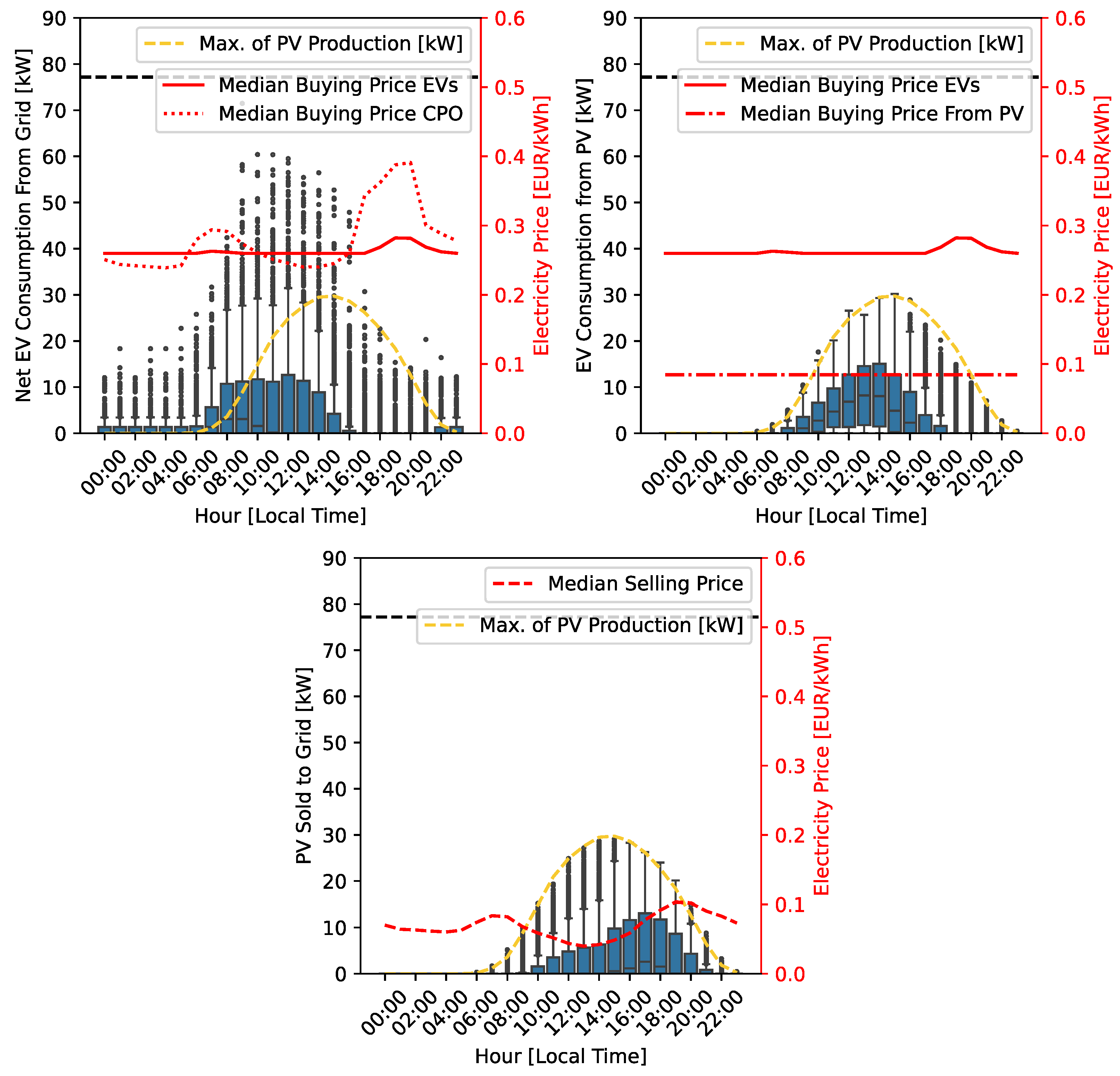
5.3. S5 & S6—PV-Powered Costs-Based Centralised Optimisation Results

S5 and S6 made use of the available production from a 35 kWp rooftop PV system installed on a nearby building to reduce both the EV charging and CPO provision costs. The EV charging patterns in S5 are presented in Figure 16 for the case of costs minimisation.

The main difference between S5 and S6 was how much the EV owners paid to absorb from the PV system: in S5, they only paid the LCOE of the PV system (EUR 0.085/kWh EUR/kWh), while in S6 they paid 99% of the regular electricity cost, a value which mathematically ensured that the PV production was consumed before the EVs started absorbing from the grid. In short, S5 and S6 represented extreme cases where the PV production was priced in a way that benefited mostly the EV owners (S5) or the CPO (S6). As the daily charging pattern for S6 was similar to S5, it will not be reported, for the sake of brevity. The left plot in Figure 16 shows the net EV load, i.e., the power that was absorbed by the EVs after they consumed the available PV production. Indeed, since the minimum cost of purchase was EUR 0.26/kWh from the grid and EUR 0.085/kWh from the PV system (LCOE), the EVs would always consume the available PV production first, as shown in the right plot of Figure 16. Finally, the bottom plot shows the energy sold to the grid by the CPO. Note how the remuneration of the PV injection was very low (around EUR 0.05–0.09/kWh), while each kWh consumed from the PV system saved the CPO EUR 0.25–0.4 and the EV owners EUR 0.26. Note that the PV production peaked at 14:00 local time (GMT + 2 in summer) because the PV system was not optimally oriented to S but slightly to SW; hence, the peak shifted to a later time of the day. The results from Table 3 show that using a PV system without SC reduced the CPO provision costs from EUR 13.24k/year (S3) to either EUR 7.06k/year (S5) or EUR 4.37k/year (S6). These reductions were even stronger when SC was applied, as the costs in S5 and S6 lowered to EUR 5.09k/year and EUR 1.44k/year, respectively. Thus, the CPO costs were reduced by 28–67% when PV-powered costs-based SC was applied. In terms of the payback period, if the PV system had to be installed ad hoc, its CAPEX of EUR 43750 (considering the EUR 1250/kWp mentioned in Section 4.2) would be recovered in 3.7–5.5 years with a 0% discount rate. The EV owners benefited from the PV system as well, in the case of the CPO deciding to have them pay the LCOE only (S5). Indeed, costs with SC reduced from EUR 10.17k/year to EUR 9.08k/year, a 10.70% reduction compared to the case of UC. The emissions reduction was less relevant for S5 and S6, but the application of SC still showed 3.5% lower emissions than UC.

Sensitivity Analysis for S6

In order to understand the impact of the installed PV capacity and the average number of EV charging sessions per day happening in the parking lot, we present the results of a sensitivity analysis that considered the same assumptions as S6 (cost-based SC with a discount if EVs were charged; without a discount for charging with the PV production), but modifying either the installed PV capacity or the number of charging events happening. The reason why we chose S6 was that it represented the best-case scenario for the CPO, which owned the PV system, while slightly reducing the charging costs for the EV owners. The results are presented in Figure 17 and Figure 18.

Figure 17 shows that the net revenues for the CPO increased if higher PV capacities were installed, thanks to the proposed SC strategy. More specifically, a reduction of around EUR 750/year in electricity provision costs was achieved when installing 80 kWp of PV instead of 30 kWp (current situation), with an average saving of around EUR 15/kWp. The EV owners charging cost, which decreased the CPO revenues, stably reduced by around EUR 200/year, while the revenue from the sold PV energy, which contributed to increasing the CPO net revenues, decreased by EUR 270/year. These elements combined into a CPO net revenue increase of around EUR 1500–2100/year (20–30%), i.e., EUR 25–50/year/kWp. It is notable how the savings tended to saturate as the installed PV capacity increased, which happened because the parking lot usage was too low and, thus, the PV energy needed to be sold instead of consumed, which was the least economically viable outcome.

Figure 18 instead, shows that if the average number of charging sessions/day increased from the current value of 7, up to 27 sessions/day (2.25 sessions/day/EVSE), the CPO provision costs savings would increase by 1500 €/year, despite the EV owners charging cost savings and PV revenue decrease reaching up to 750 €/year. These values translate into a net revenue increase for the CPO of around 2500–3500 €/year (30–35%). The evident saturation of these values shown in Figure 18 as the number of session increases is quite indicative of the fact that, considering the current EV energy requirements and connection times, there is a limit in the usage of the parking lot at around 2 sessions/charger. After that, elements such as parking space availability and queuing times need to be considered.

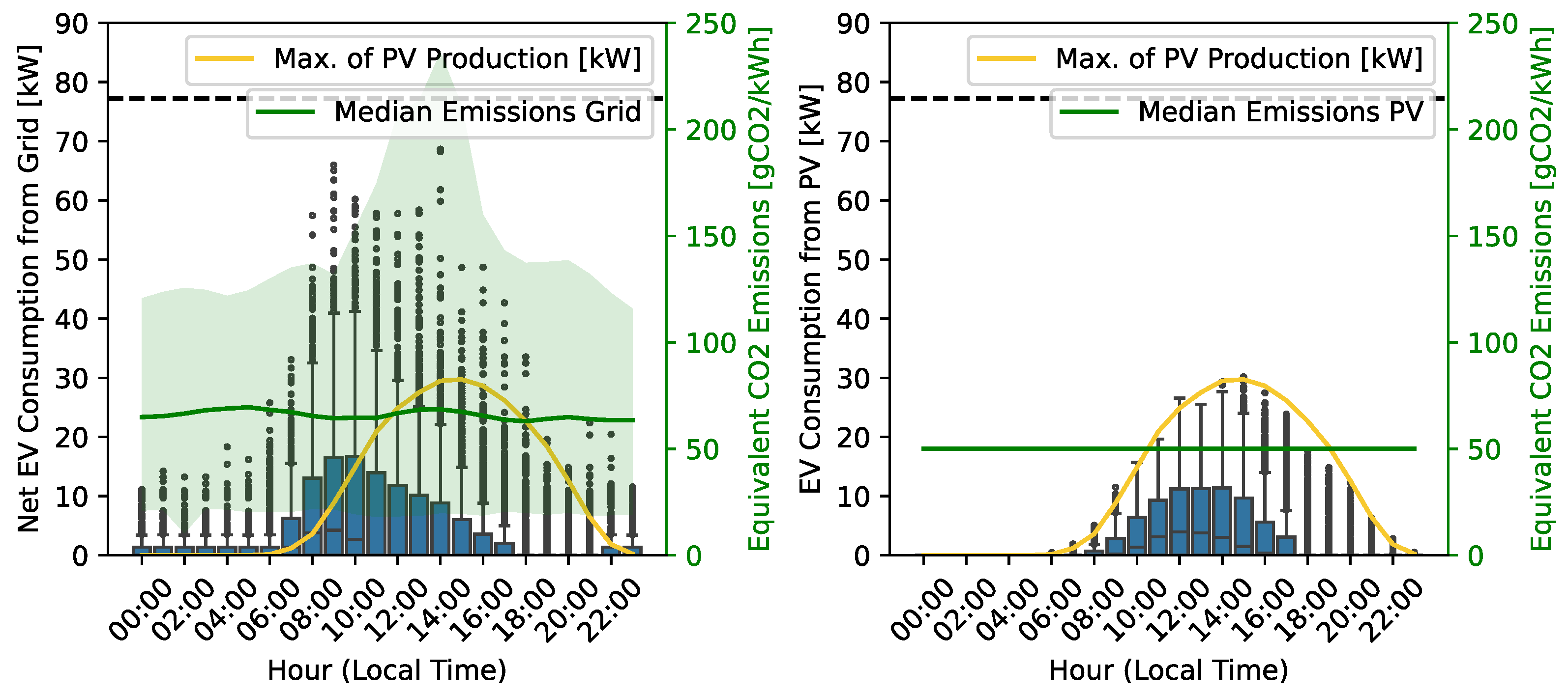
5.4. S7 & S8—PV-Powered Emissions-Based Centralised Optimisation Results

S7 and S8 made use of the available PV production from the PV system to minimize the CO₂ emissions from the cluster operation. The EV charging patterns of S7 are shown in Figure 19. The charging patterns of S8 were identical to the ones of S7, so, for the sake of brevity, they will not be reported. Since the CO₂ emissions from the grid had a median of 69 gCO₂/kWh—which is typical for systems with a high penetration of renewables, like Denmark—the SC algorithm would still prefer to charge the EVs from the grid whenever the grid emissions were lower than the 50 gCO₂/kWh considered for the PV system. Adopting a conservative approach, we assumed no negative emission coefficients when injecting PV power into the system.

Once again, the EV charging consumption was localised when the PV system was producing (08:00–21:00). Whenever it was not possible to use the PV production or the grid energy had a lower carbon content than the one produced by the PV system, the EVs consumed from the grid, avoiding the increased variability from 12:00 to 14:00. Our numerical results show that the PV system had a very positive impact on the CO₂ emissions, with a 470 kgCO₂/year reduction compared to S4. SC decreased the CO₂ emissions further, by another 240 kg/year. Costs-wise, S8 was more profitable for the CPO, since the EV owners paid the full price of electricity when absorbing from the PV system, with SC leading to a 16.50% CPO provision costs reduction over SC. S7 was, instead, the most profitable scenario for the EV owners, with a 2.7% costs reduction thanks to the application of SC. Overall, we can conclude that, due to the high penetration of renewables (wind) energy in the Danish grid, charging based on emissions is not the most efficient way of using SC.

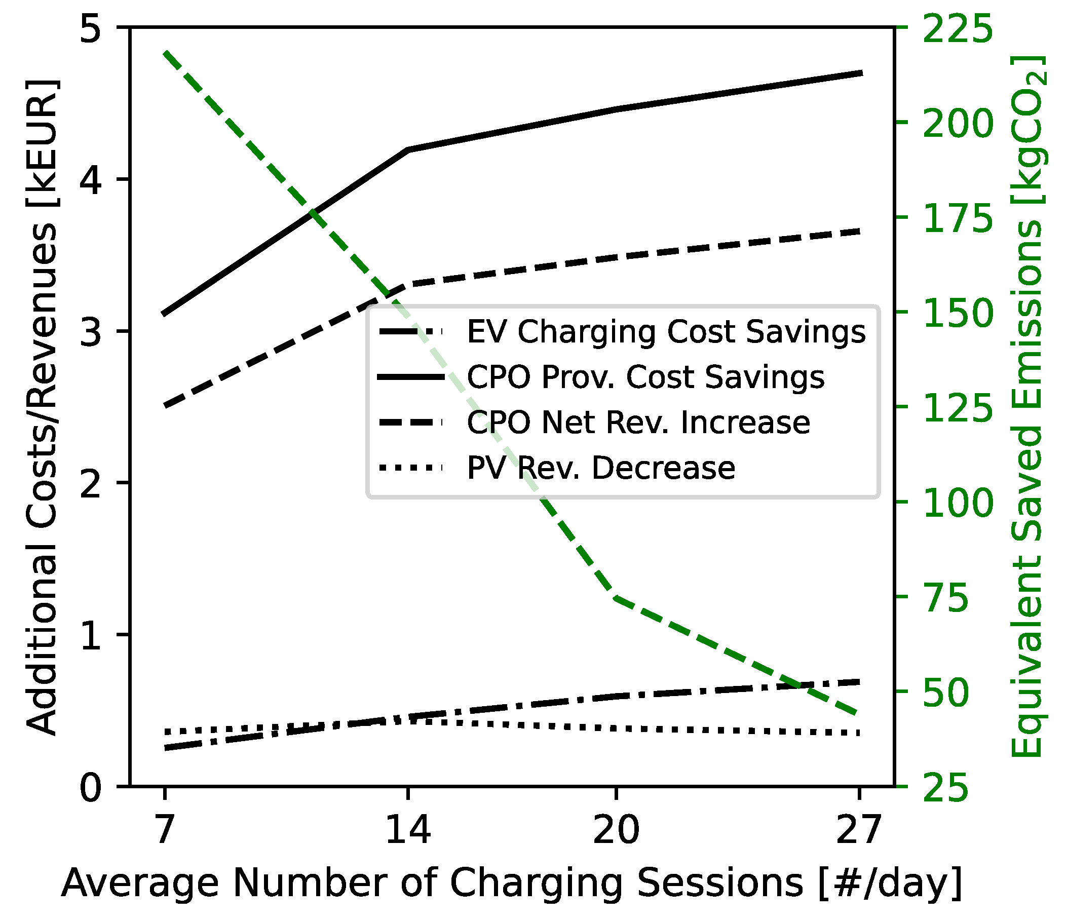
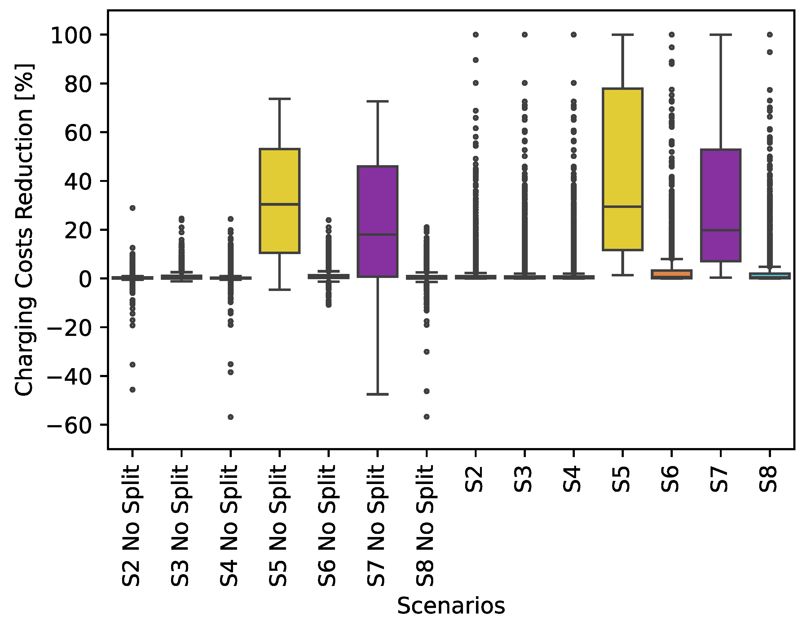
5.5. Benefit-Splitting Algorithm Impact

In S1, the decentralised cost-based SC scenario, the optimizer already made sure each session was cheaper/had less emissions when SC was applied. In all the other ones, i.e., in S2–S8, the global economic savings from SC needed to be redistributed between the participating EV owners, to ensure that everyone was well-off. Our results with and without applying the benefit-splitting algorithm from Section 3.3 are shown in Figure 20 as the percentage reduction in charging costs compared to UC $\Delta cos{t}_{n,REL}$, as described in Equation (26) for each EV owner.

From Figure 20, it is notable how in S2, S3, S4, S6, S7, and S8 some EV owners experienced cost increases by up to 70% compared to UC. This can happen for several reasons: for example, (i) SC tries to minimise the global emissions but increases the charging cost, in turn, (ii) the costs minimisation includes the CPO provision costs too, and that interferes with the minimisation of the EV charging costs, (iii) an EV owner who would naturally charge at a certain time is delayed in an SC scenario, due to other EVs queuing up and reducing the total available charging capacity in the parking lot. In these cases, the benefit-splitting algorithm ensured that the daily money savings achieved by all the EVs collectively were split so that everyone was saving money at the end of the charging session, with the biggest saving assigned to the most delayed EV first, then prioritising the EV owners with the lowest SC benefit. The median per-EV saving was around 20–30% for S5 and S7, the most profitable cases for the EV owners, and close to zero for all the other cases.

6. Conclusions

In this paper, we propose a centralised V1G control algorithm for a cluster of EV chargers in a parking lot, able to exploit the production from a nearby rooftop PV system and respect realistic constraints regarding EV operating conditions. We also propose an algorithm to split the benefits of smart charging between the EV owners, based on the delay they experience in charging their vehicles. The key findings of this work can be summarised as follows:

• Due to the minimum charging cost limit and the low price variability during EV connection hours, EV scheduling based on cost without a PV system was not profitable in the analysed parking lot (up to 1.1% cost reduction for the EV owners, and 2.7% for the CPO). It was more efficient to minimise based on the CO₂ emissions (5.60% emissions reduction).
• The inclusion of an already-existing PV system led to the highest cost and emission savings (up to 11% for the EV owners and 67% for the CPO). Assuming the most CPO-friendly smart charging scenario, savings of around EUR 1500–2100/year (20–30%) could be realised with 30–80 kWp of installed PV capacity by implementing the proposed smart charging strategy. These values could reach EUR 2500–3500/year (30–35%) if the usage of the parking lot was increased from its current value to an average of two sessions/day per charging station.
• The centralised algorithm was able to quickly and efficiently reduce the peak charging power from the cluster; hence, the parking lot fuse capacity could be reduced from 68.3 to 40 kW with minimal unserved energy issues and a substantial cost reduction for the CPO.
• The SC benefits need to be reallocated to make sure the EV owners do not lose money from centralised SC. The algorithm we propose ensures no economic losses and splits the benefits based on the experienced delay.

Future research directions will entail (i) the analysis of V2G schemes, where EVs can be discharged to perform energy arbitrage, (ii) the provision of peak reduction as a service to the grid operator in the form of a of “conditional” connection agreement between the CPO and the grid operator, and (iii) a detailed economic analysis of the profitability for a newly installed PV system to feed the EVs.

References

1. Xia, X.; Li, P. A review of the life cycle assessment of electric vehicles: Considering the influence of batteries. Sci. Total Environ. 2022, 814, 152870. [Google Scholar] [CrossRef]
2. IEA. Global EV Outlook 2024; International Energy Agency: Paris, France, 2024. [Google Scholar]
3. Secchi, M.; Barchi, G.; Macii, D.; Petri, D. Smart electric vehicles charging with centralised vehicle-to-grid capability for net-load variance minimisation under increasing EV and PV penetration levels. Sustain. Energy Grids Netw. 2023, 35, 101120. [Google Scholar] [CrossRef]
4. Engelhardt, J.; Malkova, A.; Cao, X.; Zunino, P.; Zepter, J.M.; Ziras, C.; Marinelli, M. EV4EU D2.3—Optimal Management of V2X in Parking Lots; Technical Report; Technical University of Denmark: Kongens Lyngby, Denmark, 2024. [Google Scholar]
5. Qian, K.; Fachrizal, R.; Munkhammar, J.; Ebel, T.; Adam, R. Large-scale EV charging scheduling considering on-site PV generation by combining an aggregated model and sorting-based methods. Sustain. Cities Soc. 2024, 107, 105453. [Google Scholar] [CrossRef]
6. Luo, J.; Yuan, Y.; Joybari, M.M.; Cao, X. Development of a prediction-based scheduling control strategy with V2B mode for PV-building-EV integrated systems. Renew. Energy 2024, 224, 120237. [Google Scholar] [CrossRef]
7. Luo, J.; Cao, X.; Yuan, Y. Comprehensive techno-economic performance assessment of PV-building-EV integrated energy system concerning V2B impacts on both building energy consumers and EV owners. J. Build. Eng. 2024, 87, 109075. [Google Scholar] [CrossRef]
8. Khalid, M.; Thakur, J.; Bhagavathy, S.M.; Topel, M. Impact of public and residential smart EV charging on distribution power grid equipped with storage. Sustain. Cities Soc. 2024, 104, 105272. [Google Scholar] [CrossRef]
9. Palmiotto, F.; Zhou, Y.; Forte, G.; Dicorato, M.; Trovato, M.; Cipcigan, L.M. A coordinated optimal programming scheme for an electric vehicle fleet in the residential sector. Sustain. Energy Grids Netw. 2021, 28, 100550. [Google Scholar] [CrossRef]
10. Park, K.; Moon, I. Multi-agent deep reinforcement learning approach for EV charging scheduling in a smart grid. Appl. Energy 2022, 328, 120111. [Google Scholar] [CrossRef]
11. Tveit, M.H.; Sevdari, K.; Marinelli, M.; Calearo, L. Behind-the-Meter Residential Electric Vehicle Smart Charging Strategies: Danish Cases. In Proceedings of the 2022 International Conference on Renewable Energies and Smart Technologies, REST 2022, Tirana, Albania, 28–29 July 2022. [Google Scholar] [CrossRef]
12. Board, A.; Sun, Y.; Huang, P.; Xu, T. Community-to-vehicle-to-community (C2V2C) for inter-community electricity delivery and sharing via electric vehicle: Performance evaluation and robustness analysis. Appl. Energy 2024, 363, 123054. [Google Scholar] [CrossRef]
13. Karimi-Arpanahi, S.; Jooshaki, M.; Pourmousavi, S.A.; Lehtonen, M. Leveraging the flexibility of electric vehicle parking lots in distribution networks with high renewable penetration. Int. J. Electr. Power Energy Syst. 2022, 142, 108366. [Google Scholar] [CrossRef]
14. Daryabari, M.K.; Keypour, R.; Golmohamadi, H. Robust self-scheduling of parking lot microgrids leveraging responsive electric vehicles. Appl. Energy 2021, 290, 116802. [Google Scholar] [CrossRef]
15. Sørensen, L.; Morsund, B.B.; Andresen, I.; Sartori, I.; Lindberg, K.B. Energy profiles and electricity flexibility potential in apartment buildings with electric vehicles—A Norwegian case study. Energy Build. 2024, 305, 113878. [Google Scholar] [CrossRef]
16. Srithapon, C.; Månsson, D. Predictive control and coordination for energy community flexibility with electric vehicles, heat pumps and thermal energy storage. Appl. Energy 2023, 347, 121500. [Google Scholar] [CrossRef]
17. Amry, Y.; Elbouchikhi, E.; Gall, F.L.; Ghogho, M.; Hani, S.E. Optimal sizing and energy management strategy for EV workplace charging station considering PV and flywheel energy storage system. J. Energy Storage 2023, 62, 106937. [Google Scholar] [CrossRef]
18. Jadoun, V.K.; Sharma, N.; Jha, P.; Jayalakshmi, N.S.; Malik, H.; Márquez, F.P.G. Optimal Scheduling of Dynamic Pricing Based V2G and G2V Operation in Microgrid Using Improved Elephant Herding Optimization. Sustainability 2021, 13, 7551. [Google Scholar] [CrossRef]
19. Sadati, S.M.B.; Moshtagh, J.; Shafie-khah, M.; Rastgou, A.; Catalão, J.P. Operational scheduling of a smart distribution system considering electric vehicles parking lot: A bi-level approach. Int. J. Electr. Power Energy Syst. 2019, 105, 159–178. [Google Scholar] [CrossRef]
20. Cao, X.; Ziras, C.; Engelhardt, J.; Marinelli, M. Distributed control of electric vehicle clusters for user-based power scheduling. In Proceedings of the ITEC Asia-Pacific 2023—2023 IEEE Transportation Electrification Conference and Expo, Asia-Pacific, Chiang Mai, Thailand, 28 November–1 December 2023. [Google Scholar] [CrossRef]
21. Abdalla, M.A.A.; Min, W.; Bing, W.; Ishag, A.M.; Saleh, B. Double-layer home energy management strategy for increasing PV self-consumption and cost reduction through appliances scheduling, EV, and storage. Energy Rep. 2023, 10, 3494–3518. [Google Scholar] [CrossRef]
22. Dik, A.; Kutlu, C.; Sun, H.; Calautit, J.K.; Boukhanouf, R.; Omer, S. Towards sustainable urban living: A holistic energy strategy for electric vehicle and heat pump adoption in residential communities. Sustain. Cities Soc. 2024, 107, 105412. [Google Scholar] [CrossRef]
23. Montes, T.; Batet, F.P.; Igualada, L.; Eichman, J. Degradation-conscious charge management: Comparison of different techniques to include battery degradation in Electric Vehicle Charging Optimization. J. Energy Storage 2024, 88, 111560. [Google Scholar] [CrossRef]
24. Bibak, B.; Bai, L. An optimization approach for managing electric vehicle and reused battery charging in a vehicle to grid system under an electricity rate with demand charge. Sustain. Energy Grids Netw. 2023, 36, 101145. [Google Scholar] [CrossRef]
25. Li, J.; Wang, G.; Wang, X.; Du, Y. Smart charging strategy for electric vehicles based on marginal carbon emission factors and time-of-use price. Sustain. Cities Soc. 2023, 96, 104708. [Google Scholar] [CrossRef]
26. Guo, G.; Gong, Y. Energy management of intelligent solar parking lot with EV charging and FCEV refueling based on deep reinforcement learning. Int. J. Electr. Power Energy Syst. 2022, 140, 108061. [Google Scholar] [CrossRef]
27. Heinisch, V.; Göransson, L.; Erlandsson, R.; Hodel, H.; Johnsson, F.; Odenberger, M. Smart electric vehicle charging strategies for sectoral coupling in a city energy system. Appl. Energy 2021, 288, 116640. [Google Scholar] [CrossRef]
28. Bartolini, A.; Comodi, G.; Salvi, D.; Østergaard, P.A. Renewables self-consumption potential in districts with high penetration of electric vehicles. Energy 2020, 213, 118653. [Google Scholar] [CrossRef]
29. Zhang, L.; Alvarez, E.M.O.; Huang, P. Optimizing coordinated spatio-temporal control of electric vehicles for enhanced energy sharing and performance across building communities. Energy Build. 2024, 312, 114167. [Google Scholar] [CrossRef]
30. Gong, J.; Wasylowski, D.; Figgener, J.; Bihn, S.; Rücker, F.; Ringbeck, F.; Sauer, D.U. Quantifying the impact of V2X operation on electric vehicle battery degradation: An experimental evaluation. eTransportation 2024, 20, 100316. [Google Scholar] [CrossRef]
31. Shi, J.; Zeng, T.; Moura, S. Electric fleet charging management considering battery degradation and nonlinear charging profile. Energy 2023, 283, 129094. [Google Scholar] [CrossRef]
32. Thingvad, A.; Ziras, C.; Marinelli, M. Economic value of electric vehicle reserve provision in the Nordic countries under driving requirements and charger losses. J. Energy Storage 2019, 21, 826–834. [Google Scholar] [CrossRef]
33. IEC 60947-2; Low-Voltage Switchgear and Controlgear—Part 2: Circuit-Breakers. International Electrotechnical Committee (IEC): Geneva, Switzerland, 2019.
34. Prina, M.G.; Lionetti, M.; Manzolini, G.; Sparber, W.; Moser, D. Transition pathways optimization methodology through EnergyPLAN software for long-term energy planning. Appl. Energy 2019, 235, 356–368. [Google Scholar] [CrossRef]
35. Boyd, S.; Vandenberghe, L. Convex Optimization; Cambridge University Press: Cambridge, UK, 2004. [Google Scholar] [CrossRef]
Figure 1. Schematic depiction of the centralised algorithm execution logic. The algorithm is run every time t * an EV connects to or disconnects from the parking lot.
Smartcities 08 00112 g001
Figure 2. Schematic depiction of the communication infrastructure in the parking lot. All the arrows represent information flows, data is read every time t * the optimisation is run.
Smartcities 08 00112 g002
Figure 3. Flowchart of the overall SC scheduling and savings splitting process. Smart charging happens in real-time, billing and benefit splitting is daily, final compensation is monthly/yearly. UC = Uncontrolled Charging (no SC).
Smartcities 08 00112 g003
Figure 4. Sky view of the charging cluster on the campus of the Technical University of Denmark (DTU). The parking lot is located in an urban area surrounding the city of Copenhagen.
Smartcities 08 00112 g004
Figure 5. Statistical distribution of the energy charged per session/EV.
Smartcities 08 00112 g005
Figure 6. Total energy charged per day in the cluster with respect to the day of the week. Dots represent outliers of the analysed statistical distributions. The dots represent the outliers of the analysed statistical distributions.
Smartcities 08 00112 g006
Figure 7. Statistical distribution of the arrival, power stop, and departure instants during the day. The different shades of each colour represent the overlapping parts of the histograms.
Smartcities 08 00112 g007
Figure 8. Statistical distribution of the maximum charging power measured for each session.
Smartcities 08 00112 g008
Figure 9. Charging pattern during the day in the recorded period in the “Uncontrolled Charging” (UC) baseline scenario. Median EV charging and CPO provision costs are reported, together with the median and interquartile range of the CO2 emissions for the electricity coming from the network. The dots represent the outliers of the analysed statistical distributions.
Smartcities 08 00112 g009
Figure 10. Average hourly dynamic charging prices for the EV owners across the optimised period.
Smartcities 08 00112 g010
Figure 11. Average hourly dynamic charging prices for the CPO across the optimised period.
Smartcities 08 00112 g011
Figure 12. Daily charging pattern when decentralised cost-based EV charging optimisation is applied. The dots represent the outliers of the analysed statistical distributions.
Smartcities 08 00112 g012
Figure 13. Daily charging pattern when decentralised CO2 emission optimisation is applied. The dots represent the outliers of the analysed statistical distributions.
Smartcities 08 00112 g013
Figure 14. Daily power distribution when a centralised cost-based optimisation was applied. The dots represent the outliers of the analysed statistical distributions.
Smartcities 08 00112 g014
Figure 15. Daily power distribution when a centralised emissions-based optimisation was applied. The dots represent the outliers of the analysed statistical distributions.
Smartcities 08 00112 g015
Figure 16. Daily power distribution for S5, which used the centralised SC algorithm and benefited from an existing 35 kWp PV system. The dots represent the outliers of the analysed statistical distributions.
Smartcities 08 00112 g016
Figure 17. Sensitivity analysis results for the economic value of SC, with respect to the installed PV capacity. Simulations were based on the same assumptions as S6.
Smartcities 08 00112 g017
Figure 18. Sensitivity analysis results for the economic value of SC, with respect to the average number of EV charging sessions/day. Simulations were based on the same assumptions as S6.
Smartcities 08 00112 g018
Figure 19. Daily power distribution for S7, which used the centralised SC algorithm and benefited from an existing 35 kWp PV system. The dots represent the outliers of the analysed statistical distributions.
Smartcities 08 00112 g019
Figure 20. Charging cost reduction per session ( Δ c o s t n , R E L S C ) for the different analysed scenarios. S3–S8 are presented without the SC benefit split as well. The dots represent the outliers of the analysed statistical distributions.
Smartcities 08 00112 g020