Advanced Wind Speed Forecasting: A Hybrid Framework Integrating Ensemble Methods and Deep Neural Networks for Meteorological Data

Highlights

What are the main findings?

• Multivariate forecasting models that incorporate multiple meteorological variables improve accuracy over univariate approaches.
• Hyperparameter optimization and walk-forward cross-validation confirm the robustness of ET and LSTM models for wind speed prediction.

What is the implication of the main finding?

• Incorporating diverse weather features and tuning models carefully enhances practical forecasting in complex Andean terrains.
• The framework offers a scalable and data-driven approach for wind-related planning in energy, infrastructure, and disaster risk contexts.

Abstract

The adoption of wind energy is pivotal for advancing sustainable power systems, particularly in off-grid microgrids where infrastructure limitations hinder conventional energy solutions. The inherent variability of wind generation, however, challenges grid reliability and demand–supply balance, necessitating accurate forecasting models. This study proposes a hybrid framework for short-term wind speed prediction, integrating deep learning (Long Short-Term Memory, LSTM) and ensemble methods (random forest, Extra Trees) to exploit their complementary strengths in modeling temporal dependencies. A multivariate approach is adopted using meteorological data (including wind speed, temperature, humidity, and pressure) to capture complex weather interactions through a structured time-series design. The framework also includes a feature selection stage to identify the most relevant predictors and a hyperparameter optimization process to improve model generalization. Three wind speed variables, maximum, average, and minimum, are forecasted independently to reflect intra-day variability and enhance practical usability. Validated with real-world data from Cuenca, Ecuador, the LSTM model achieves superior accuracy across all targets, demonstrating robust performance for real-world deployment. Comparative results highlight its advantage over tree-based ensemble techniques, offering actionable strategies to optimize wind energy integration, enhance grid stability, and streamline renewable resource management. These insights support the development of resilient energy systems in regions reliant on sustainable microgrid solutions.

1. Introduction

Each year, the increasing demand for electricity presents a formidable challenge to our power infrastructure. Wind energy emerges as a promising solution to reduce the carbon footprint associated with electricity generation. In recent years, the installed wind capacity has seen a remarkable surge, reaching an impressive 769.196 MW by the year 2021, as reported by IRENA (the International Renewable Energy Agency) [1].

Wind energy, considered a pivotal component of the renewable energy landscape, has garnered significant academic and technical interest owing to its sustainability, environmental consciousness, and contributions to energy security. However, the widespread integration of wind farms into power systems presents formidable challenges due to the stochastic and intermittent nature of wind as an energy source. These challenges encompass strategic wind farm siting and sizing, daily energy scheduling, power quality management, and ensuring grid system stability and reliability, all while accommodating the inherent variability and uncertainty of wind generation. These complexities underscore the imperative for comprehensive research and technical solutions in the context of integrating wind energy within contemporary power systems.

Wind speed is considered one of the most challenging weather parameters to model and forecast due to its random and intermittent nature [2]. Therefore, it becomes crucial to utilize effective wind power forecasting tools to promote the installation of wind farms. Several methods have been proposed in the literature, primarily categorized into conventional methods and Artificial Intelligence (AI).

Traditional approaches for wind power forecasting often rely on stochastic time series analysis and multivariate regression models. For example, the study by [3] introduces an innovative statistical framework that integrates an evaluation of meteorological forecast reliability, using this metric as a corrective factor in predictive models. This approach proved effective for operational management of power grids with high wind energy integration and for optimizing bids by wind farm operators in energy markets. Experimental validation, using historical production data from an operational wind farm, demonstrated that quantifying uncertainties in atmospheric variables significantly enhances the accuracy of short- and medium-term power output predictions. The authors of [4] propose a locally feedback dynamic fuzzy neural network (LF-DFNN) with enhanced representation, local modeling, and stable learning for wind speed prediction in wind farms, outperforming other models. In [5], a generic framework is introduced for probabilistic energy forecasting, employing multiple quantile regression, an efficient optimization method, and a radial basis function network, showcasing successful applications in various energy tracks. The authors of [6] study a novel framework, CE-MOLS, combining complete ensemble empirical mode decomposition, monarch butterfly optimization, and Long Short-Term Memory to enhance the accuracy of very short-term wind power generation prediction. Experimental results show a significant improvement over benchmark models. In [7], a new statistical approach enhances short-term wind-electric power forecasts for wind power plants using wind-pattern recognition, adaptive boosting, and machine learning with reference wind mast data. The proposed model outperforms benchmark and conventional statistical methods by 2.3% to 5.1% in normalized Mean Absolute Error. The authors of [8] tackle Day-Ahead Wind Power Forecasting, providing high-resolution intra-period wind variability predictions. It introduces a Wasserstein distance-based loss, proving superior accuracy through comparisons and market data evaluation.

Among artificial intelligence (AI) techniques, deep learning methods stand out for their ability to process and analyze large datasets effectively, making them highly suitable for complex forecasting tasks. These methods include Convolutional Neural Networks (CNNs), Recurrent Neural Networks (RNNs), and Reinforcement Learning (RL) [9], among others. Additionally, other AI approaches such as Artificial Neural Networks (ANNs) [7] and Support Vector Machines (SVMs) [10] have also been widely applied, demonstrating their versatility in various predictive modeling scenarios. Convolutional methods play a significant role in numerous studies due to their effectiveness in handling complex data patterns. For instance, the authors of [11] propose a hybrid approach that integrates elastic variational mode decomposition with forecasting random convolution nodes, significantly improving the accuracy of wind speed time-series forecasting, especially for Gaussian heteroscedastic data. Similarly, in [12], a novel framework for wind power forecasting is explored, which combines a graph convolution network (GCN) with the maximum information coefficient (MIC) to capture spatial dependencies, alongside a multiresolution Convolutional Neural Network (CNN) to model temporal features. This combined approach has been shown to enhance the precision of short-term wind power predictions. In the context of forecasting wind time series, Convolutional Neural Networks (CNNs) excel in capturing spatial features relevant to the data’s geographical layout, while Recurrent Neural Networks (RNNs) are well-suited for capturing sequential dependencies over time in wind speed patterns. The authors of [13] propose a hybrid method for wind speed forecasting, using elastic variational mode decomposition and forecasting random convolution nodes, demonstrating improved accuracy for Gaussian heteroscedastic time-series data through evaluation on an actual dataset. In [14], the study tackles the challenges posed by weather variability in wind power generation. The authors propose an innovative approach using a hedge backpropagation-based online Long Short-Term Memory (LSTM) architecture, specifically designed for ultra-short-term wind power prediction. This method outperforms conventional algorithms in terms of accuracy, offering valuable support for the efficient operation and management of wind farms.

The use of advanced artificial intelligence and statistical modeling has really transformed wind speed prediction lately. Studies have found that deep learning models can leverage past weather data to deliver short-term forecasts with greater accuracy than conventional techniques [15]. This type of approach not only improves predictive capabilities but also allows for better planning in wind farms, as is the case in the study conducted at Baron Techno Park, where its applicability in real scenarios was validated. Conversely, reference [16] investigated the application of probabilistic generative models to gauge both wind speed and the electrical output from wind farms. This technique brings in an extra layer of controlled uncertainty, which plays a vital role in decision-making when it comes to managing the balance between energy supply and demand. Additionally, these authors have pointed out the importance of utilizing multivariable neural networks to refine short-term weather forecasts, particularly those related to the height of wind turbine hubs. This approach helps to minimize prediction errors by making dynamic adjustments based on historical data. Also, reference [17] has come up with an innovative approach by introducing the MIESTC model, which is a multivariable spatiotemporal system. This model smartly integrates geographic and temporal information to boost the accuracy of very short-term forecasts. It highlights how blending spatial and temporal analysis can break through the limitations of methods that rely solely on time, especially when navigating the complex wind patterns that vary across different geographical areas. However, despite the advances, significant limitations still persist in this area of research. Many of the studies mentioned use historical data with low temporal resolution or that are limited to specific areas, which restricts the generalization of the models. They do not take advantage of current AI tools that allow the extraction of specific and relevant characteristics of the wind model to more accurately model a system. Likewise, some approaches lack an analysis of air speed variability, where there are low, medium, and high speed contexts that affect various environments, such as renewable energy generation.

The aforementioned studies offer valuable insights and innovative approaches to forecasting wind energy generation, particularly focusing on univariate predictive models. It is also relevant to emphasize that these works make an important use and analysis of features such as future selection that allow taking into account all the most relevant characteristics of a model to make an adequate prediction of its output variables, which leaves several opportunities at the research level to improve the prediction processes of techniques and algorithms.

While many existing works rely on single-variable inputs, this study introduces a more comprehensive strategy by employing multivariate machine learning techniques. Specifically, it explores the use of Extremely Randomized Trees (ET) and Long Short-Term Memory (LSTM) networks to capture the complex interactions among multiple meteorological variables influencing wind speed and power generation. To further improve model accuracy and generalization, both models are subjected to a structured hyperparameter optimization process. This combination of multivariate input and optimized modeling enhances the robustness and precision of short-term wind speed forecasting, ultimately supporting the reliable integration of wind energy into sustainable power systems.

The main contributions of this study are as follows:

• A comprehensive comparative analysis of traditional, machine learning, and deep learning models for wind speed forecasting in a South American highland context. This study includes both univariate and multivariate model configurations, allowing for a systematic assessment of performance under real meteorological conditions.
• A multioutput prediction framework is proposed, in which separate models are trained to forecast maximum, average, and minimum wind speed. This approach reflects the temporal variability of wind behavior throughout the day and improves the practical relevance of forecasts for risk assessment, operational planning, and energy generation.
• The evaluation includes four types of models: Persistence (PER), Autoregressive (AR), Extremely Randomized Trees (ET), and Long Short-Term Memory (LSTM) networks. The two best-performing models, ET and LSTM, are further assessed using 10-fold walk-forward validation, providing statistically grounded insights into their reliability and generalization.
• The role of meteorological predictors is examined through an embedded feature importance analysis, aiding interpretability and reducing model complexity. While not the central contribution, this analysis ensures a compact and efficient model input space, tailored to the Andean region of Ecuador.

This paper is organized as follows: Section 2 presents the methodology used in the research, detailing the algorithms and predictive techniques focused on wind speed. Section 3 describes the case study based on data collected in the city of Cuenca, Ecuador. Section 4 includes a detailed analysis of the results obtained, along with their discussion. Finally, Section 5 outlines the main conclusions derived from this work.

2. Methodology

For the development of the predictive model, data collected by a VAISALA meteorological station located on the campus of the Universidad Politécnica Salesiana in Cuenca, Ecuador, were used. The recorded data include relevant meteorological variables, which were previously processed and organized for analysis.

To identify the most influential features in wind speed prediction, a random forest-based feature selection technique was applied. Subsequently, several predictive models were trained and evaluated, considering both univariate and multivariate approaches, with the aim of comparing their performance in short-term forecasting. The implemented models included deep neural networks of the Long Short-Term Memory (LSTM) type, as well as ensemble methods such as the Extra Trees (ET) model.

Model performance was assessed using standard metrics, including the Root Mean Square Error (RMSE), Mean Absolute Error (MAE), Mean Absolute Percentage Error (MAPE), and the coefficient of determination (R²). These metrics enabled an objective comparison among the different approaches analyzed.

2.1. Multivariate Time Series Modeling for Wind Speed

The multivariate temporal model used to model the wind speed data (in

Table 1. Variables.

Variable	Type of Data	Abbreviation
Maximum solar irradiance	Numerical (${\displaystyle \frac{\mathrm{W}}{{\mathrm{m}}^2}}$)	MaxSI
Average solar irradiance	Numerical (${\displaystyle \frac{\mathrm{W}}{{\mathrm{m}}^2}}$)	AvgSI
Minimum solar irradiance	Numerical (${\displaystyle \frac{\mathrm{W}}{{\mathrm{m}}^2}}$)	MinSI
Maximum air temperature	Numerical (°C)	MaxAT
Average air temperature	Numerical (°C)	AvgAT
Minimum air temperature	Numerical (°C)	MinAT
Maximum relative humidity	Numerical (%)	MaxRH
Average relative humidity	Numerical (%)	AvgRH
Minimum relative humidity	Numerical (%)	MinRH
Maximum barometric pressure	Numerical (hPa)	MaxBP
Average barometric pressure	Numerical (hPa)	AvgBP
Minimum barometric pressure	Numerical (hPa)	MinBP
Maximum wind speed	Numerical (${\displaystyle \frac{\mathrm{m}}{\mathrm{s}}}$)	MaxWS
Average wind speed	Numerical (${\displaystyle \frac{\mathrm{m}}{\mathrm{s}}}$)	AvgWS
Minimum wind speed	Numerical (${\displaystyle \frac{\mathrm{m}}{\mathrm{s}}}$)	MinWS
Wind direction	Numerical (°)	WD
Precipitation	Numerical (mm)	Precipt

) can be formalized as

$${\widehat{y}}^t=f\left(X_v^t\right)=f(X_1^t,X_2^t,\dots ,X_v^t),$$

(1)

where $X_i^t$ denotes the temporal input variables and ${\widehat{y}}_t$ corresponds to the model’s predicted output at time t. It is important to highlight that the temporal model is multivariate in nature, meaning that wind speed predictions are based on multiple time-dependent variables. Each variable is influenced not only by its own historical values but also exhibits interdependencies with other variables. These relationships are leveraged to improve the accuracy of forecasting future wind speed values, as the model captures the complex interactions and correlations between the variables over time. This multivariate approach enhances the predictive capability of the model by incorporating a more comprehensive representation of the underlying dynamics. The expression in Equation (1) can be represented in matrix form to emphasize the multidimensional structure of the temporal input, where X$=X_v^t,\mathrm{for}v\in \{1,\dots ,16\}$, corresponds to the temporal variables detailed in Table 1. Considering the time-dependent characteristics of the dataset utilized in the model, Equation (1), can be written as

$${\widehat{y}}^{t+1}=f\left({\mathbf{X}}^{\mathbf{t}},{\mathbf{X}}^{\mathbf{t}-\mathbf{1}},\dots ,{\mathbf{X}}^{\mathbf{t}-\mathbf{k}}\right),$$

(2)

where $t\in \{1,\dots ,N-k\},\left\{{\mathbf{X}}^{\mathbf{t}},{\mathbf{X}}^{\mathbf{t}-\mathbf{1}},\dots ,{\mathbf{X}}^{\mathbf{t}-\mathbf{k}}\right\}$. Within this analytical framework, the matrix ${\mathbf{X}}^t$ captures temporal patterns from past and present data points in the sequence, whereas ${\widehat{y}}^{t+1}$ indicates the model’s projected outcome. The function f serves as the core predictive algorithm, parameter k specifies the temporal range employed for prediction calculations, and N reflects the total quantity of annual records in the dataset. Note that the indexing corresponds to the temporal dimension t. For the sake of simplicity, the variable index v has been omitted, resulting in the matrix representation depicted in Equation (2).

2.2. Persistence (PER) Model

The utilization of the Persistence model serves as a fundamental reference point for evaluating the efficacy of the machine learning models. This methodology offers a valuable approach for establishing a foundational prediction baseline for temporal data patterns. The central idea involves projecting that the forthcoming time step will replicate the value of the preceding time step. Essentially, this involves forecasting that the value at time $t+1$ will precisely align with the actual value recorded at time t [18].

2.3. Autoregressive (AR) Model

The Autoregressive model is a method for predicting future values within time series analysis. It achieves this by calculating predictions through a linear combination of historical data points. This approach is founded on the belief that a variable’s forthcoming values are connected to its own preceding values.

Within the AR model, the forecast for the target variable at a specific time is created by analyzing its previous values from earlier times. The choice of lag order determines how many past data points, or the size of the historical window, are considered when formulating predictions [19]. The selection of the lag order for the Autoregressive (AR) model was based on information criteria, specifically the Akaike Information Criterion (AIC) and Bayesian Information Criterion (BIC), which balance model fit and complexity. The optimal lag corresponds to the value that minimizes these criteria across candidate models [20].

The standard representation of an Autoregressive model with a lag parameter k, expressed as AR(k), is defined by the following formulation:

$$\widehat{y}={\widehat{x}}_t={\beta }_0+{\beta }_1{x}_{t-1}+{\beta }_2{x}_{t-2}+\dots +{\beta }_p{x}_{t-k}+{\epsilon }_t$$

(3)

In this notation system, the following are used:

• $x_t$ indicates the variable’s measurement at period t;
• $x_{t-1},x_{t-2},\dots ,x_{t-k}$ denote delayed instances of $x_t$ with maximum lag p, reflecting the variable’s prior states;
• The constant ${\beta }_0$ defines the model’s intercept value under zero predictor conditions, addressing systemic data offsets;
• Parameters ${\beta }_1,\dots ,{\beta }_k$ measure how historical values proportionally affect current results;
• The stochastic component ${\epsilon }_t$ captures unmodelled variability at timestep t, including all random disturbances.

2.4. Long Short-Term Memory

Architectures based on Long Short-Term Memory (LSTM) are highly proficient at analyzing and deriving knowledge from sequential data. Unlike vanilla Recurrent Neural Networks (RNNs) plagued by vanishing and exploding gradients, LSTMs overcome these limitations by incorporating gating mechanisms and internal memory units that selectively control the flow of information, which are listed as follows [21].

Forget Gate ($f_t$) Determines which information from the previous cell state ($C_{(t-1)}$) to discard.

$$f_t=\sigma (W_f·[h_{t-1},x_t]+b_f)$$

(4)

The mechanism employs a sigmoid function ($\sigma$) to produce outputs constrained within the range of 0 to 1. Values approaching 1 suggest that the information is preserved, whereas those nearing 0 imply that the information is discarded.

Input Gate ($i_t$) Regulates which parts of the current input ($x_t$) to integrate into the cell state.

$$i_t=\sigma (W_i·[h_{t-1},x_t]+b_i)$$

(5)

Mirroring the behavior of the forget gate, this component utilizes a sigmoid activation function ($\sigma$) to generate outputs within the 0 to 1 range. A higher value allows more information from the current input to flow into the cell state, while a lower value restricts it.

Output Gate ($o_t$) Controls what portion of the updated cell state ($C_t$) is exposed to the network’s output ($h_t$).

$$o_t=\sigma (W_o·[h_{t-1},x_t]+b_o)$$

(6)

Uses the sigmoid activation function ($\sigma$) for values between 0 and 1. A higher value reveals more information from the updated cell state to the network, while a lower value hides most of it.

Transformed Input Vector (${\tilde{C}}_t$) Function: Provides candidate information for updating the cell state.

$${\tilde{C}}_t=tanh(W_C·[h_{t-1},x_t]+b_C)$$

(7)

Uses a hyperbolic tangent activation function (tanh) to output values between −1 and 1. This vector serves as a potential update for the cell state, modulated by the input gate.

2.5. Extremely Randomized Trees or Extra Trees (ET) Model

The Extra Trees model is a formidable ensemble learning technique within the family of decision tree-based algorithms. What sets the Extra Trees model apart is its distinctive approach to feature selection during each node split [22].

Unlike traditional decision trees, the Extra Trees model introduces a high degree of randomness by randomly selecting features for each node split. This heightened randomness serves to amplify the diversity among individual decision trees, making them more unique. This increased randomness within the model results in a one-of-a-kind combination of decision trees. While this introduces additional variance, it effectively curbs overfitting, a common challenge when dealing with intricate and noisy data. Ultimately, the Extra Trees model arrives at its final prediction by aggregating the predictions of all individual trees within the ensemble as ${\widehat{Y}}_{\mathrm{ET}}={\displaystyle \frac{1}{N_T}}{\sum }_{i=1}^{N_T}{\widehat{Y}}_i$. In this context, the following are used: ${\widehat{Y}}_{\mathrm{ET}}$ represents the ensemble’s predicted value. ${\widehat{Y}}_i$ signifies the forecasted value from the ith decision tree within the Extra Trees ensemble. $N_T$ is the total count of decision trees that compose the Extra Trees ensemble.

2.6. Research Workflow

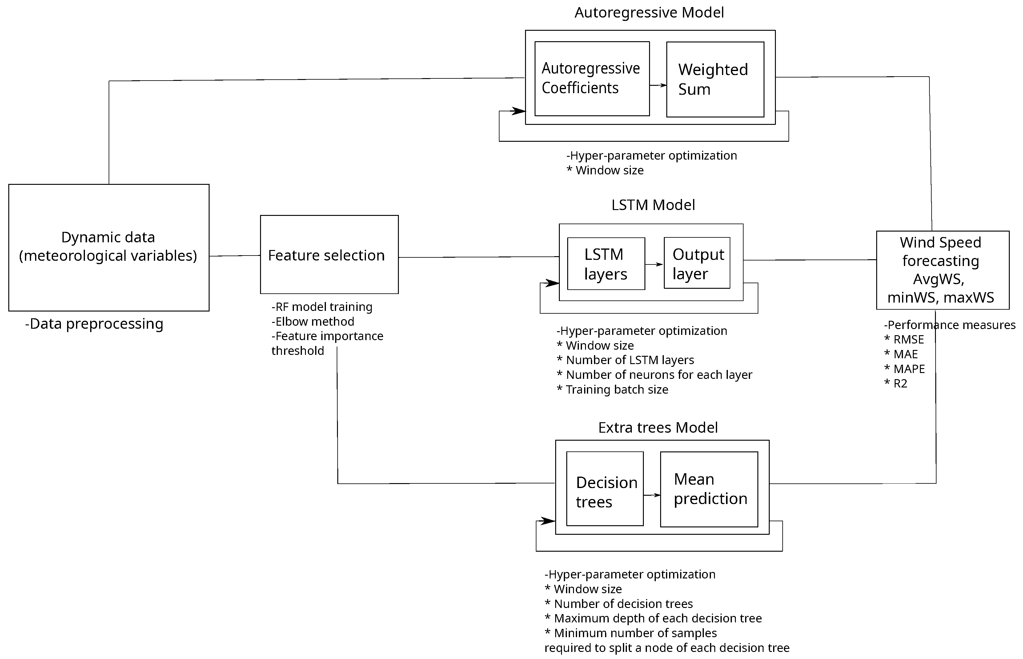
The multimodel framework offers an opportunity to explore the distinct strengths of various methods in system modeling. There are studies, such as those by [23,24,25,26,27], that have adopted such frameworks; however, none have implemented a decentralized approach that leverages different information analysis techniques. The process of wind speed prediction encompasses several steps, which can be delineated as follows:

Data preparation: The process begins with the identification and correction of missing values in the dataset, with special attention given to selecting a time interval that has the least amount of data loss. Once cleaned, the data are divided into two subsets: a training set used for model development and a testing set reserved for performance evaluation and validation of the models.

AR reference model: As a reference, two base models are implemented: the Persistence model (PER) and the Autoregressive model (AR). The PER model assumes that the next wind speed value will be equal to the most recent observed value, serving as a naïve but commonly used benchmark in time series forecasting. The AR model, on the other hand, is a linear model that predicts wind speed based on its past values. Together, these baseline models provide a foundation for evaluating the added value of more complex machine learning and deep learning approaches, allowing for a comprehensive comparison of forecasting accuracy.

Feature selection: To determine which input variables are most relevant for wind speed forecasting, a random forest model is used to compute feature importance scores. This technique evaluates the contribution of each meteorological variable to the prediction task. Based on these results, the most informative variables are selected to train the advanced models, reducing noise and improving model focus.

Model training and hyperparameter tuning: Both the LSTM and Extremely Randomized Trees (ET) models are trained using the training dataset. During this process, hyperparameter tuning is performed to find the most effective configuration for each model. This tuning step helps enhance the models’ predictive accuracy and generalization capability by adjusting parameters such as learning rate, tree depth, number of units, and others specific to each algorithm.

Model evaluation: After training and optimization, the models are evaluated using the testing dataset. Their predictive performance is measured using several common evaluation metrics, including the Coefficient of Determination (R²), Mean Absolute Error (MAE), Mean Absolute Percentage Error (MAPE), Root Mean Square Error (RMSE), and Standard Deviation Error (SDE). These metrics provide a comprehensive view of each model’s strengths and limitations.

This full process is summarized schematically in Figure 1.

3. Case Study

Database and Normalization

The methodological framework for atmospheric data acquisition in this research employed a VAISALA weather station as the primary sensor array, coupled with a QML201C data logger for continuous recording at 10-min temporal resolution. System control and data standardization were implemented via VAISALA HydroMet™ Automatic Weather Station Client Software (AWS Client), ensuring systematic archiving of meteorological parameters. Positioned in an exposed environment, the weather station continuously records meteorological data, including barometric pressure, relative humidity, solar irradiation, temperature, wind direction, and wind speed, among others. These parameters are measured using various sensors, including a Rain Gauge Tipping Bucket for precipitation, an Ultrasonic Anemometer for wind, a probe HMP155 and HUMICAP 180R sensor for temperature and humidity, a Hukseflux thermal sensor SR11 for solar irradiation, and a Vaisala Barocap BARO-1 for barometric pressure. Meteorological measurements are routed to a desktop computing unit operating the proprietary VAISALA HydroMet™ AWS Client software, featuring an interactive visualization platform for data collection and processing. Records are captured hourly and remain available for analytical workflows. Figure 2 depicts the position of the instrumentation at coordinates (−2.8867, −78.9903) within the campus of Universidad Politécnica Salesiana (Cuenca, Azuay, Ecuador). Collected data are stored in CSV format after conversion from the original log files and are described in Table 1.

After inspecting the quality of the data, it was decided to work only with the data generated in the years 2015 and 2016, which allowed us to avoid a majority of null values as seen in

Table 2. Statistical information of solar irradiance variables (W/m²).

Variable	Dataset	Max	Median	Min	Mean	St.d
MaxWS	Total dataset	17.40	5.50	0.60	5.99	3.26
	Train dataset	17.30	5.60	0.70	5.98	3.19
	Test dataset	17.40	5.50	0.60	5.99	3.51
AvgWS	Total dataset	9.00	2.50	0.00	2.63	1.68
	Train dataset	9.00	2.50	0.00	2.64	1.64
	Test dataset	8.60	2.30	0.00	2.57	1.84
MinWS	Total dataset	3.00	0.00	0.00	0.21	0.37
	Train dataset	3.00	0.00	0.00	0.22	0.37
	Test dataset	2.50	0.00	0.00	0.17	0.34

.

Figure 3 shows the hourly variation of wind speed in Cuenca using boxplots for each hour of the day. The data reveal a clear diurnal pattern: wind speeds are lower during the early morning hours (00:00–07:00), then increase steadily, peaking between 13:00 and 16:00, before gradually declining again into the evening. This pattern is consistent with daytime heating and atmospheric mixing processes that typically increase wind activity during the day. The spread (interquartile range) also increases during these peak hours, indicating greater variability in wind speed. Given the observed variability in wind speed, both throughout the day and across different months, it becomes essential to predict not only the average wind speed but also the maximum and minimum scenarios. Together, these three metrics provide a more complete understanding of wind behavior, which is critical for applications such as risk assessment, renewable energy optimization, and infrastructure resilience. Figure 4 presents the monthly variation of wind speed throughout the year. Wind speeds appear relatively stable across months, but August and June show slightly higher median and upper quartile values, suggesting stronger and more variable winds during these months. Conversely, March, April, and October exhibit lower median wind speeds. The boxplots also highlight the presence of outliers in most months, indicating occasional high wind speed events. Together, these figures provide useful temporal insights for understanding intraday and seasonal wind behavior, which is essential for accurate forecasting and planning in renewable energy applications.

4. Results and Discussion

4.1. Feature Selection

Before model training was conducted, a feature selection technique was used to retain only the most valuable variables. This technique involves identifying and extracting the most pertinent and informative features from a larger set. This procedure assists in directing the model’s focus toward the most critical aspects of the data, resulting in predictions that are both more precise and resource-efficient.

A random forest algorithm was utilized for this task due to its ability to handle high-dimensional data [28,29,30]. In the training process of the RF model, the methodology revolved around incorporating all variables as inputs, except for wind speed. The target variable for prediction was the AvgWS. Notably, the decision to exclude the variables MaxWS and MinWS was motivated by their redundancy, as they essentially communicated the same information.

In order to enhance the model’s performance, a randomized hyperparameter search was executed. The objective of this method is to discover the most advantageous combination of hyperparameter values by randomly selecting from a predefined search space. The choice to utilize the random search approach was motivated by the goal of quickly gaining valuable insights.

After training the RF model with optimized hyperparameters, it gains the ability to reveal the relative importance of each feature. The procedure for ascertaining feature importance entails assessing the extent to which a particular feature diminishes the level of randomness present in data subsets. The greater the reduction attributed to a feature, the greater its importance in aiding accurate predictions or classifications within the model.

To retain the most valuable features for the prediction models, a threshold was established based on the mean importance score. Only features surpassing this threshold were chosen for inclusion in the multivariate models. This method allowed for the prioritization of the most influential variables while upholding model simplicity.

Figure 5 presents the ranked importance of the predictor variables, with a red dashed line representing the mean importance value used as a reference threshold. While this threshold is useful for its simplicity and interpretability, the most notable aspect of the plot is the clear elbow pattern observed in the distribution of feature importances. This elbow behavior provides a more visually grounded criterion for selecting the most influential variables, highlighting a natural cutoff point that supports the choice of key predictors. The variables identified at the elbow include maximum solar irradiance (MaxSI), wind direction (WD), and maximum relative humidity (MaxRH), which not only exceed the mean importance threshold but also correspond to the point where the curve begins to flatten. This alignment with the inflection point reinforces their relevance and supports their selection as the most important predictors for the model.

In addition to the selected features, the subsequent models incorporated both MaxWS and MinWS as input variables. This approach aims to encompass all valuable information necessary for predicting wind speed.

Figure 6 presents a correlation matrix (left) and the corresponding Variance Inflation Factor (VIF) scores (right) for the meteorological variables used in this study. Notably, MaxWS, MinWS, and AvgWS show high pairwise correlation, particularly between MaxWS and MinWS ($\rho \sim 0.91$) which is expected given that these variables represent different aspects of wind speed distribution over an hour and are derived from the same underlying 10-min resolution data. In time series modeling, these three variables are often used in combination as rolling statistical summaries, capturing different dynamics of wind behavior across short intervals. Their inclusion is especially relevant in hourly models where temporal granularity must be preserved without oversimplifying the variability of the signal [31].

While the VIF values for MaxWS (9.9) and MinWS (8.4) are relatively high, they remain below common critical thresholds (e.g., VIF > 10) and reflect the natural multicollinearity arising from their shared origin. Importantly, for models such as LSTM and Extremely Randomized Trees (ET), multicollinearity is not a limiting factor for performance, as these models are designed to learn complex nonlinear dependencies and are not sensitive to linear redundancy. Additionally, since the objective of this work is forecasting rather than interpretation, even in traditional Autoregressive models, the presence of moderate multicollinearity does not pose a significant issue. Thus, the retention of MaxWS, MinWS, and AvgWS is justified both methodologically and contextually within a robust time series forecasting framework.

4.2. LSTM Model Training

The training of the LSTM model encompassed a grid search methodology aimed at identifying the optimal hyperparameters. This approach systematically examined all possible combinations within a predefined set of choices.

The main goal was to achieve the lowest RMSE. To achieve this, multiple hyperparameters were selected for optimization, including:

• Window size: The number of preceding observations or time intervals considered when predicting future events. The selected values were 26, 28, and 30.
• Number of neurons: The quantity of neurons present in each LSTM layer. The values considered during exploration were 50, 75, and 100 neurons.
• Batch size: It denotes the quantity of data instances that the model processes and learns from before updating its parameters. The selected values for this parameter were 50, 100, and 150.
• Number of LSTM layers: This hyperparameter dictates the quantity of LSTM layers incorporated into the model. The values considered in this analysis included 1, 2, and 3.

By systematically investigating all the options specified in the grid search, a total of 81 combinations were evaluated.

Table 3. Optimal Hyperparameters on Univariate LSTM Model.

Output Variable	Window Size	Number of Neurons	Batch Size	LSTM Layers	RMSE
MaxWS	26	100	150	2	1.34
AvgWS	30	50	50	3	0.85
MinWS	28	75	50	3	0.27

displays the optimal hyperparameter configuration for all univariate LSTM models.

Figure 7 depicts the progression of the minimum RMSE for the univariate LSTM model. MaxWS modeling achieved peak performance with a temporal window spanning 26 time steps, 100 neural units per LSTM layer, training batches containing 150 samples, and a two-layer stacked LSTM architecture.

AvgWS forecasting demonstrated optimal results using an input sequence length of 30 intervals, a 50-node configuration across individual LSTM layers, a mini-batch configuration of 50 instances, and a three-tiered LSTM structure.

MinWS projections yielded superior accuracy with a 28-unit historical window, 75 computational nodes per hidden LSTM layer, batch processing with 50 entries, and a triple-layer LSTM topology.

Similarly, the multivariate LSTM models were subjected to testing using a total of 81 combinations.

Table 4. Optimal Hyperparameters on Multivariate LSTM Model.

Output Variable	Window Size	Number of Neurons	Batch Size	LSTM Layers	RMSE
MaxWS	28	100	100	1	1.20
AvgWS	28	100	150	2	0.72
MinWS	28	50	150	2	0.25

presents the optimal hyperparameters for these models, while Figure 8 illustrates the progression of the minimum RMSE across different hyperparameter sets.

For MaxWS prediction, the optimal hyperparameter configuration included a 28-unit historical window, 100 neural units, a training batch size of 100, and a single-layer LSTM architecture.

Regarding AvgWS forecasting, the minimal RMSE was attained using a 28-step input sequence, 100 neurons per layer, a batch size of 150, and a two-layer LSTM framework. Finally, when forecasting MinWS, the optimal hyperparameters included a window size of 28, 50 neurons, a batch size of 150, and the implementation of 2 LSTM layers.

4.3. ET Model Training

The optimization process for the ET model followed the same approach as that used for optimizing the LSTM model. The hyperparameters selected for this optimization comprised the following:

• Window size: A range of different temporal windows were explored for the ET model. Continuing with the LSTM process, an identical set of choices was implemented, consisting of timeframes of 26, 28, and 30 h in the past.
• Maximum depth: This parameter sets the upper limit on the depth of individual trees within the random forest. The values considered for evaluation were 10, 20, 40, and 80.
• Number of estimators: This hyperparameter controls the total quantity of decision trees integrated into the random forest model. The values tested during optimization were 100, 200, and 300.
• Minimum samples for node splitting: This setting defines a critical criterion, determining the smallest number of samples necessary within a node to permit further partitioning while building the decision trees. The values examined for this parameter were 2, 5, and 10.

Taking into account all possible hyperparameter combinations, a total of 108 configurations were assessed for the ET models. The optimal hyperparameters for both univariate and multivariate models are detailed in

Table 5. Optimal Hyperparameters on Univariate ET Model.

Output Variable	Window Size	Maximum Depth	Number of Estimators	Min Samples Split.	RMSE
MaxWS	30	20	300	10	1.32
AvgWS	28	20	200	10	0.84
MinWS	28	10	300	2	0.27

and

Table 6. Optimal Hyperparameters on Multivariate ET Model.

Output Variable	Window Size	Maximum Depth	Number of Estimators	Min Samples Split.	RMSE
MaxWS	28	40	300	2	1.22
AvgWS	28	40	300	5	0.72
MinWS	26	20	200	10	0.25

, respectively. Additionally, Figure 9 and Figure 10 offer visual representations of the progression of the minimum RMSE in both scenarios.

The univariate modeling approach attained peak performance for MaxWS forecasting using a 30-unit historical window, a tree depth limit of 20, 300 ensemble estimators, and a node splitting threshold of 10 samples.

For AvgWS prediction, the highest accuracy was achieved with a 28-step input sequence, a maximum depth constraint of 20, 200 decision trees, and a minimum of 10 samples per node.

In the case of MinWS estimation, the most effective configuration utilized a 28-interval window, a depth restriction of 10, 300 estimators, and a node division requirement of 2 samples.

Conversely, when all selected variables are incorporated into the prediction process, the ideal configuration for predicting MaxWS comprises a window size of 28, a maximum depth of 40, 300 estimators, and a minimum sample count of 2. For predicting AvgWS, the best settings are a window size of 28, a maximum depth of 40, 300 estimators, and a minimum sample count of 5. For MinWS forecasting, the ideal parameter combination includes a 26-unit historical window, a tree depth limit of 20, 200 ensemble estimators, and a node splitting threshold of 10 samples.

4.4. Comparing Model Outcomes

All the models were trained using the freely accessible Google Colab platform. This platform dynamically allocates computational resources based on availability, which may introduce some variability in the time required for model optimization. Nevertheless, it is still possible to make meaningful comparisons. The findings indicated that the ET model had the quickest optimization time, whereas the LSTM models necessitated approximately ten times more time for optimization. To ensure transparency and reproducibility, the complete implementation, including data processing, feature selection, model training, and hyperparameter tuning, is available in a public GitHub repository [32].

Following the optimization of the models,

Table 7. Performance Evaluation of Optimized Models.

Output Variable	Model	RMSE (${\displaystyle \frac{\mathbf{m}}{\mathbf{s}}}$)	MAE (${\displaystyle \frac{\mathbf{m}}{\mathbf{s}}}$)	MAPE (%)	R2
MaxWS	PER	1.64	1.18	19.19	0.78
	AR	1.35	0.99	16.87	0.85
	Univariate ET	1.33	0.98	16.73	0.86
	Univariate LSTM	1.35	0.98	16.30	0.85
	Multivariate ET	1.22	0.89	15.09	0.88
	Multivariate LSTM	1.21	0.89	15.26	0.88
AvgWS	PER	1.00	0.71	22.47	0.70
	AR	0.87	0.62	21.42	0.78
	Univariate ET	0.85	0.62	21.50	0.79
	Univariate LSTM	0.86	0.63	22.00	0.78
	Multivariate ET	0.72	0.54	18.74	0.85
	Multivariate LSTM	0.72	0.54	18.86	0.85
MinWS	PER	0.33	0.17	12.04	0.06
	AR	0.28	0.18	13.92	0.34
	Univariate ET	0.28	0.18	13.83	0.34
	Univariate LSTM	0.28	0.18	14.29	0.34
	Multivariate ET	0.26	0.16	12.98	0.42
	Multivariate LSTM	0.24	0.15	10.92	0.45

presents a comparison of their predictive performance on the test dataset. The evaluation metrics include the coefficient of determination (R2), Root Mean Squared Error (RMSE), Mean Absolute Error (MAE), and Mean Absolute Percentage Error (MAPE).

The results clearly demonstrate the superiority of the multivariate models in wind speed prediction. In the context of MaxWS forecasting, the multivariate LSTM model attained the lowest RMSE, measuring at 1.21 m/s, closely trailed by the multivariate ET model, which achieved an RMSE of 1.22 m/s. This signifies an improvement of approximately 26% in comparison with the baseline PER model, which recorded an RMSE of 1.64 m/s. Furthermore, there was a reduction of 10% in comparison to the AR model, which yielded an RMSE of 1.35 m/s. It is noteworthy that the univariate models, both ET and LSTM, achieved RMSE values very close to the performance of the AR model, with 1.33 m/s and 1.35 m/s, respectively.

In the context of predicting AvgWS, both multivariate models, LSTM and ET, achieved an identical RMSE of 0.72 m/s. This signifies an improvement of approximately 28% compared with the PER model, which obtained an RMSE of 1 m/s. Furthermore, both multivariate models outperformed the AR model, which had an RMSE of 0.87 m/s, which represents an improvement of approximately 17%. Similar to the previous scenario, the univariate models exhibited similar error rates to the AR model. The univariate LSTM model yielded an RMSE of 0.86 m/s, while the univariate ET model recorded an RMSE of 0.85 m/s.

Finally, in the case of MinWS prediction, the multivariate LSTM model achieved the lowest RMSE, measuring at 0.24 m/s, closely followed by the multivariate ET model with an RMSE of 0.26 m/s. This signifies an improvement of approximately 27% compared with the PER model, which yielded an RMSE of 0.33 m/s. Additionally, it represents an improvement of roughly 14% when compared with the AR model, which had an RMSE of 0.28 m/s. It is noteworthy that both univariate models produced the same RMSE as the AR model. Moreover, it is crucial to highlight that the R2 value of 0.06 obtained by the PER model indicates an exceptionally weak relationship with the data, reflecting minimal predictive capacity. In striking contrast, the top-performing model, the multivariate LSTM, achieved an R2 of 0.45. This marks a substantial increase in prediction accuracy.

To ensure robust model evaluation while respecting the temporal structure of the data, walk-forward validation was employed. A technique specifically designed for time series forecasting tasks. Unlike standard k-fold cross-validation, which assumes data points are independent and identically distributed, walk-forward validation maintains the chronological order of observations. In this approach, the model is trained on an initial window of historical data and validated on the immediately following time segment. The training window then expands forward (or slides, depending on the strategy), and the process is repeated across multiple folds. This method mimics real-world forecasting conditions where only past data are available for model training and future data are reserved for testing, thereby avoiding data leakage and providing a more realistic estimate of predictive performance [33].

Figure 11 presents a comparison of prediction performance for MinWS, AvgWS, and MaxWS using two selected models: a multivariate LSTM and an Extremely Randomized Trees (ET) regressor. The results are based on Root Mean Square Error (RMSE) values obtained through a 10-fold time series split (walk-forward validation), and are visualized using violin plots to show the distribution and variability across folds. Overall, both models exhibit stable and consistent performance across the three target variables. Slightly lower RMSE values are observed for MaxWS, while AvgWS shows greater variability in prediction error. The analysis highlights the robustness of both LSTM and ET for short-term wind speed forecasting. Notably, the LSTM model tends to outperform ET, especially for MinWS and AvgWS, as indicated by higher quartile boundaries in the violin plots. These findings support the effectiveness of the LSTM architecture in capturing temporal dependencies in multivariate wind speed data.

It is worth noting that the average error obtained through the 10-fold walk-forward validation procedure is lower than the error observed on the final validation set in Table 7. This behavior is expected in time series forecasting, as walk-forward validation evaluates the model across multiple, temporally ordered subsets of the data, each with progressively larger training histories. In contrast, the final validation set represents a single, held-out segment at the end of the time series, which may include more recent or volatile patterns that are harder to predict. Additionally, models in walk-forward validation are retrained for each fold using updated training data, potentially benefiting from recent temporal context, while the final test prediction relies on a fixed training window. As such, this difference in error highlights the importance of using both validation strategies to gain a comprehensive understanding of model performance over time and under varying conditions.

4.5. Visualization of Time Series Forecasting Results

Figure 12 offers a graphical representation of the comparative analysis between model predictions and actual data for a reserved validation test set. In the graphical representation, the x-axis (horizontal) denotes observed values, whereas the y-axis (vertical) displays the predicted outputs produced by the respective models. A diagonal red line within the plot indicates the ideal correspondence between measured and forecasted values. Additionally, in the plot, different symbols are utilized to distinguish between univariate and multivariate models: blue dots are used to indicate predictions generated by univariate models, while green triangles are employed to represent predictions made by multivariate models.

The models exhibit similar results when predicting MaxWS and AvgWS but face challenges when predicting MinWS. It is crucial to note that the dataset records measurements in meters per second (m/s), with a precision of 0.01 m/s between consecutive values, ranging from 0.6 to 17.40 m/s for MaxWS, from 0 to 8.60 m/s for AvgWS, and from 0 to 2.50 m/s for MinWS. As a result, the MinWS variable appears discrete in the visual representation. This discreteness is due to the narrower range of values on the X-axis compared with MaxWS and AvgWS. In practical terms, this means that MinWS typically consists of predominantly very low values with occasional spikes, making it challenging for the models to accurately estimate higher values. Consequently, the models often confine their predictions to a relatively narrow range of low values.

Figure 13 offers a comparative perspective focusing on the multivariate models, chosen for their superior performance with lower RMSE. The figure showcases a week’s worth of data, unveiling a noticeable similarity in the patterns exhibited by the models. Furthermore, the models perform well in predicting MaxWS and AvgWS. However, when it comes to MinWS, the data appear somewhat noisy, and the models struggle to predict the peaks accurately.

Finally, Figure 14 presents the complete test dataset, which has been smoothed over a monthly period. Once again, the models showcased in this figure are the multivariate models. This approach confers a distinct advantage by enhancing the clarity of trend identification.

The figure unveils distinctive patterns in the predictions of MaxWS, AvgWS, and MinWS across the models. When predicting MaxWS, it becomes evident that the LSTM model tends to generate higher values compared with the ET model, while the ET model aligns more closely with the real values. In the case of AvgWS prediction, both models exhibit remarkably similar patterns. Lastly, in the prediction of MinWS, the ET model consistently overestimates the real values, whereas the LSTM model generally aligns closely with the real values but occasionally provides lower predictions.

Finally, the histograms presented in Figure 15 demonstrate that the residuals for MinWS and AvgWS are centered near zero, with mean errors of 0.01 m/s and 0.02 m/s, respectively. This indicates that the model is effectively unbiased for these variables. In the case of MaxWS, a slight negative bias is observed, with a mean error of $-0.12$ m/s, suggesting a mild tendency to overpredict peak wind speeds. Nonetheless, the distribution of errors remains symmetric, and the 68% confidence intervals for all three variables include the zero-error line, which supports the interpretation that the model’s predictions are not systematically skewed. These visual results reinforce the reliability of the model, indicating that it maintains consistent accuracy across different wind speed targets. The overall symmetry and centering of the residual distributions around zero provide strong evidence that the multivariate LSTM model produces well-calibrated and balanced forecasts without significant systematic error.

5. Discussion and Conclusions

In this study, three distinct forecasting models were utilized to predict maximum, average, and minimum wind speeds, denoted as MaxWS, AvgWS, and MinWS. Wind speed exhibits significant variability throughout the day and across seasons, as evidenced by the hourly and monthly analyses. In this context, forecasting only a single metric, such as the average wind speed, would be insufficient to characterize the full dynamic range of wind behavior. Therefore, the proposed approach simultaneously predicts three key variables: maximum (MaxWS), minimum (MinWS), and average wind speed (AvgWS). These metrics together provide a more comprehensive understanding of wind conditions, which is critical for applications in renewable energy, environmental monitoring, and safety planning.

The predictions were made over a short-term horizon, specifically forecasting for the next hour. The chosen models included the Autoregressive (AR) model, the Long Short-Term Memory (LSTM) neural network, and the Extra Tree (ET) model. The methodology involved several key steps, including preprocessing historical meteorological data and performing feature selection to identify the most crucial climatic variables for model input. The selected variables were identified as maximum solar irradiance (MaxSI), wind direction (WD), and maximum relative humidity (MaxRH). These variables were found to contain the most valuable information necessary for accurate wind speed prediction.

Both the LSTM and ET models underwent training to forecast wind speed using two distinct approaches: univariate and multivariate. A feature selection process was guided by the mean importance threshold and the elbow criterion, identifying the most relevant meteorological predictors such as solar irradiance, wind direction, and relative humidity. Also, hyperparameter tuning was applied to both the LSTM and Extremely Randomized Trees models to maximize generalization and minimize overfitting. Overall, the findings validate the effectiveness of multivariate modeling over univariate or linear alternatives and support the use of data-driven DL/ML approaches for wind forecasting.

The results demonstrate the clear advantage of multivariate approaches. For example, in the case of MaxWS, the multivariate LSTM achieved the lowest RMSE (1.21) and highest R² (0.88), outperforming both its univariate counterpart (RMSE 1.35, R² 0.85) and traditional models like AR and PER. Similar improvements are observed across AvgWS and MinWS, where the multivariate LSTM consistently achieves lower error metrics and higher explanatory power. These results confirm that integrating related variables improves temporal modeling and forecast accuracy.

For future work, there are opportunities for research based on more complex and advanced predictive models to boost the accuracy of wind speed predictions. One key topic to explore is the use of hybrid models that blend linear and nonlinear predictors, effectively capturing both the general trends and the more hidden patterns found in meteorological data. For instance, exploring models such as ARIMA and SARIMA could enrich the baseline comparison by incorporating seasonality and differencing techniques tailored for time series. These statistical models can be used in combination with nonlinear methods such as multivariate LSTM to form hybrid forecasting architectures.

One area of research focuses on using combined deep learning models, like merging Convolutional Neural Networks (CNNs) with Long Short-Term Memory (LSTM) networks. This has shown great success in tasks that require both spatial and temporal data processing, which is particularly important for multivariate time series, such as those examined in this study. Additionally, the use of Gated Recurrent Units (GRUs), a simplified alternative to LSTM, can be investigated as they often provide competitive performance with fewer parameters. These deep models can also support automatic feature extraction, reducing dependence on manual feature selection techniques.

In addition to statistical and recurrent models, tree-based ensemble models such as random forest (RF) and their extensions can be further explored to benchmark performance and contribute to model diversity. A comparative analysis including RF alongside the multivariate LSTM and ET models would provide a broader perspective on model behavior under different data characteristics and error sensitivities.

Finally, it is suggested to explore the use of deep ensemble models, specifically stacking techniques, where multiple base models, such as CNN, LSTM, GRU, and random trees, could be combined by a meta-model that integrates their individual predictions to generate an optimized output. This approach promises to increase the robustness of the prediction system and provide better levels of generalization under varying weather conditions.