Highlights
- What are the main findings?
- This paper presents HERD-YOLO, a detection model for garbage bin overflow based on Spiking Neural Network s (SNNs). It not only achieves high accuracy in object detection but also significantly reduces energy consumption compared to traditional approaches based on artificial neural networks (ANNs).
- It also introduces the extensive Garbage Bin Status (GBS) dataset, comprising 16,771 images generated and augmented using techniques such as Stable Diffusion. This diverse dataset significantly enhances the model’s ability to generalize across various environmental conditions, including different weather and lighting scenarios.
- What is the implication of the main findings?
- The energy-efficient design of HERD-YOLO enables its deployment on resourceconstrained IoT devices, thereby making real-time waste management in smart cities more sustainable and cost effective.
- Enhanced with improved robustness and generalization capabilities, the model can accurately and promptly detect overflowing garbage bins under a wide range of realworld conditions. This ultimately facilitates smarter urban waste management and contributes to creating cleaner, healthier urban environments.
Abstract
With urbanization and population growth, waste management has become a pressing issue. Intelligent detection systems using deep learning algorithms to monitor garbage bin overflow in real time have emerged as a key solution. However, these systems often face challenges such as lack of dataset diversity and high energy consumption due to the extensive use of IoT devices. To address these challenges, we developed the Garbage Bin Status (GBS) dataset, which includes 16,771 images. Among them, 8408 images were generated using the Stable Diffusion model, depicting garbage bins under diverse weather and lighting scenarios. This enriched dataset enhances the generalization of garbage bin overflow detection models across various environmental conditions. We also created an energy-efficient model called HERD-YOLO based on Spiking Neural Networks. HERD-YOLO reduces energy consumption by 89.2% compared to artificial neural networks and outperforms the state-of-the-art EMS-YOLO in both energy efficiency and detection performance. This makes HERD-YOLO a promising solution for sustainable and efficient urban waste management, contributing to a better urban environment.
1. Introduction
As urbanization and population growth continue, the volume of waste produced by human activities increases significantly [1,2]. The mounting waste not only harms the environment but also poses health risks [3]. Therefore, effective waste management is essential. Waste management refers to the process of disposing waste in a way that safeguards the environment and human health [4,5]. Central to waste management are the temporary storage and collection of waste materials. Conventionally, waste has been temporarily stored in garbage bins, with sanitation workers tasked with collecting the waste at set intervals [6]. However, these traditional approaches are labor intensive and often fall short in the timely detection of overflowing bins [7]. The inability to ensure prompt waste removal can result in bins that overflow, leading to a host of unsanitary conditions [8]. These include the attraction of pests, the proliferation of bacteria, and the emission of unpleasant smells, all of which can significantly degrade the quality of urban environments.
To solve these problems, there arises an urgent demand for innovative approaches that can accurately detect when garbage bins reach their maximum capacity and require emptying. A particularly promising solution involves the use of intelligent detection systems [8,9,10]. These systems leverage surveillance cameras integrated with deep learning-based detection algorithms to continuously monitor garbage bins and assess the level of waste accumulation [11,12,13,14,15]. When a bin is detected to be near full capacity, the system will notify sanitation workers, thereby facilitating the timely removal of waste. By automating the monitoring process, this approach significantly improves efficiency and reduces the dependence on manual labor [16,17]. However, to the best of our knowledge, there still remain two significant challenges associated with this approach.
Firstly, the current deep learning-based models for detecting the fullness of garbage bins lack robust generalization to diverse environmental conditions. These models are primarily trained on datasets that include images or videos taken in ideal lighting and clear weather (e.g., [11,14,15]). As a result, their performance tends to deteriorate in more challenging weather scenarios, such as during rain, snow, or at night [18]. Under such circumstances, reduced visibility makes it difficult for the model to accurately detect when a bin is overflowing. This shortcoming diminishes the accuracy and practical utility of the model in real-world applications.
Secondly, the rising deployment of Internet of Things (IoT) devices for detection purposes is expected to result in a considerable increase in energy consumption [19]. This energy consumption is related to the electricity necessary for the cameras and their supporting infrastructure. With an expanding number of cameras in use, the electricity demand is likely to grow, translating into increased operational expenses. Moreover, the power consumption of these cameras might overburden local power grids, particularly during peak usage hours. Consequently, there is an urgent need to adopt more energy-efficient solutions within waste management systems to mitigate these challenges.
To tackle the aforementioned challenges, we first employ the Diffusion model [20] to expand our dataset of garbage bins. This process includes the generation of images depicting the state of garbage bins across a range of weather conditions and diverse lighting scenarios. This expansion significantly enhances the generalization ability of the model, enabling it to more adeptly handle diverse real-world situations [21]. In addition, we introduce an innovative method known as Hybrid Energy-Efficient ResDense YOLO (HERD-YOLO), which is based on the Spiking Neural Network (SNN). This approach ensures the preservation of high detection accuracy while concurrently minimizing energy consumption during hardware deployment. By enhancing both the generalization and energy efficiency of detection algorithms, our solutions could substantially improve the overall performance of garbage bin overflow detection systems.
2. Related Works
A growing number of researchers are exploring various intelligent detection systems with the aim of enhancing waste management efficacy. This section reviews the studies of assessing the occupancy rates of garbage bins using camera images.
Wang et al. [11] proposed a deep learning-based multi-task network designed for the intelligent management of garbage deposit points. They employed the YOLOv5-based approach to detect the status of garbage bins and surrounding garbage. Additionally, they integrated the Openpose [22] and Deepsort [23] algorithms to track pedestrians in the vicinity of garbage deposit points, determining if they are littering. The Insightface [24] algorithm was also utilized to record individuals who fail to comply with littering regulations.
Ramalingam et al. [25] and Gómez et al. [26] both developed deep learning-based frameworks for pavement inspection and cleaning using the self-reconfigurable robot Panthera. Both studies utilized SegNet [27] for pavement segmentation and DCNN for detecting garbage or pavement defects. The first framework was tested on Panthera with NVIDIA GPUs and MMS for geotagging, demonstrating high accuracy in identifying defects and garbage for real-time cleaning tasks. The second framework introduced a fuzzy logic-based adaptive vacuum suction scheme for efficient litter pickup and was tested with a Jetson Nano Nvidia GPU, achieving a detection time of approximately 132.2 milliseconds and a 38.5% improvement in energy consumption for pavement cleaning tasks.
Sharma et al. [14] presented a garbage bin status indicator system that employs the Convolutional Neural Networks (CNNs; [28]) model with three layers and five layers. Their models were trained on datasets obtained from CCTV camera surveillance to classify the garbage bins as either empty or full. Upon reviewing the data and results, the three-layer and five-layer CNN models achieved accuracies of 92% and 99%, respectively.
Oğuz and Ömer Faruk Ertuğrul [15] explored the application of deep learning algorithms to determine the fullness of garbage bins using camera images from the CDCM dataset [29]. Their experiments involved the application of several prominent CNN-based classification models, including DenseNet-169 [30], EfficientNet-B3 [31], MobileNetV3-Large [32], and VGG19-Bn [33]. Through a comparative analysis of these models, they achieved an accuracy rate of 94.931%, indicating the potential for intelligent systems to accurately assess the status of garbage containers.
3. Methods
3.1. Garbage Bin Status Dataset
3.1.1. Overview
We developed a dataset named the Garbage Bin Status (GBS) dataset, comprising a total of 16,771 images. Among them, 3349 images were collected from online sources and field photography, forming the base dataset. Leveraging this base, we employed the diffusion model to generate 8408 images that depict garbage bins under diverse weather and lighting scenarios. Furthermore, conventional data augmentation techniques, including geometric and color transformations, were also applied to produce an additional 5014 images. Figure 1 illustrates the distribution of these images across the three categories with a pie chart. All the images were carefully hand-labeled and subsequently applied in the training of our proposed model.
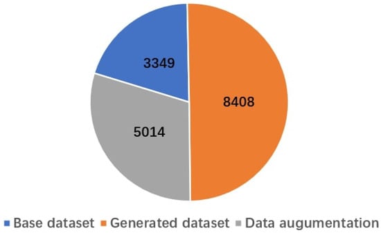
Figure 1.
A pie chart to show the image counts for the three components in the GBS dataset.
3.1.2. Base Dataset
Through leveraging both online resources and field photography, we obtained a total of 3349 images as the base dataset. Initially, we employed web crawler technology [34] to acquire a total of 2651. Some examples from the web are shown in Figure 2. In addition to the overflowing garbage bins, some garbage is often stacked outside the bins due to the large volume or other reasons, and this needs to be cleaned up as well. Therefore, our detection objectives were categorized into three distinct classes: non-overflowing garbage bins labeled as “garbage_bin”, overflowing garbage bins labeled as “overflow”, and garbage outside the bins labeled as “garbage”. The distribution of these labels within the base dataset is illustrated in Figure 3.
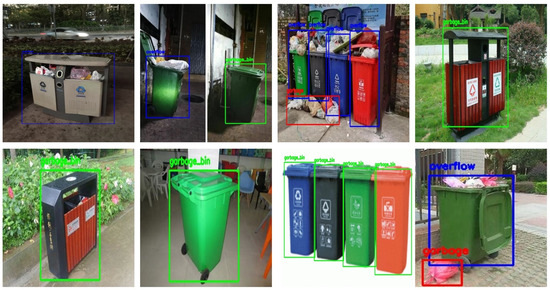
Figure 2.
Some examples of web image in the base dataset.

Figure 3.
A 100% stacked bar chart to show the percentage of labels in each of the three categories in the base dataset.
However, the number of images from the internet is limited, particularly in the categories of garbage and overflowing garbage bins, which could result in data imbalance [35]. To mitigate this issue, we turned to field photography to enrich the base dataset, focusing on taking photos of fewer categories of garbage and overflowing garbage bins. The size of the field photography images is 640 × 853 pixels. With this fieldwork, we successfully added 698 images to the base dataset. Some examples of these images are presented in Figure 4.
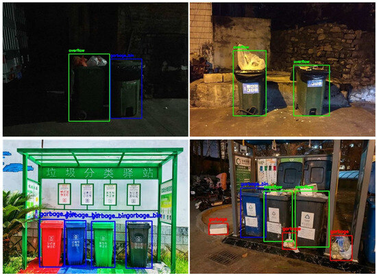
Figure 4.
Some examples of the field photography images. (The Chinese characters in the bottom-left corner of the image translates to “Waste Sorting Station”).
From the previous processes, we amassed a total of 3349 images, predominantly taken under sunny daytime conditions. In order to enhance the capability of the model for generalization, we employed the Stable Diffusion (SD) model [36] to generate additional data. This approach allows us to expand our dataset and simulate a variety of environmental contexts, thereby improving the adaptability and accuracy of the model.
3.1.3. Introduction to the SD Model
With the rapid advancement in generative modeling, especially the development of diffusion models, it has become possible to generate new data not only from existing datasets but also directly from textual prompts. The diffusion model is a cutting-edge generative model within the realm of computer vision, characterized by its capability to generate high-quality images from the noise. Among the numerous advancements in diffusion models, the SD model emerges as a standout latent diffusion model that is capable of handling a variety of tasks, including text-to-image generation, image-to-image translation, image inpainting, and image super-resolution.
The SD model functions through a pipeline that integrates three essential components: a text encoder, a latent space U-Net model, and a variational autoencoder (VAE, [37]). The text encoder leverages the Contrastive Language-Image Pre-training (CLIP, [38]) model to convert each textual token in the input prompt into an embedding vector. These embeddings along with a random noise array are then passed into the U-Net model via a cross-attention mechanism, serving as conditions for the generation process. The latent space U-Net model acts as the core of the diffusion model, tasked with the iteratively denoising process and enabling the generation of text-guided latents. The VAE is composed of two main parts: the encoder, which compresses the image into the latent space, and the decoder, which takes the latent output from the U-Net model and decodes it back into an image.
The text-to-image task refers to the process of inputting a textual prompt into the SD model, which then generates an image that matches the description of the input text. The diagram of text-to-image logical workflow of the SD model is illustrated in Figure 5. The text-to-image process begins with encoding the input prompt into embedding vectors through the CLIP text encoder, which is then fed into the diffusion model, typically U-Net, that iteratively generates the latent representation of the image from noise by aligning it with the input textual prompt. Finally, a VAE decoder reconstructs the latent image into a high-resolution, detailed picture that corresponds to the initial text description.
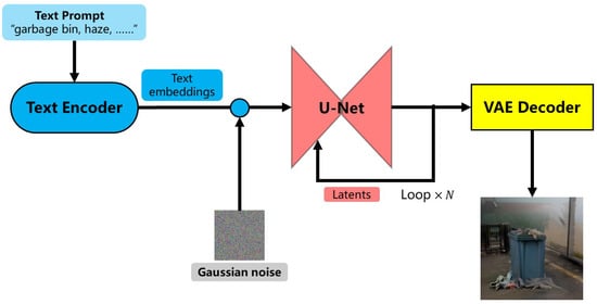
Figure 5.
Diagram of text-to-image logical workflow of the SD model.
The image-to-image task extends the text-to-image process by incorporating an additional image alongside the text prompt. The SD model then reinterprets and redraws the input image to better align it with the textual description provided. The diagram of the text-to-image logical workflow of the SD model is presented in Figure 6. Compared to the text-to-image process, the initial latent in image-to-image process is not random noise but rather the latent noise derived from encoding the input image using the VAE encoder, to which Gaussian noise is subsequently added. Beyond this step, the subsequent procedures parallel those employed in the text-to-image process.
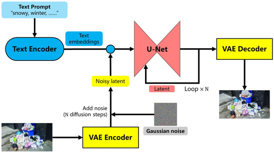
Figure 6.
Diagram of image-to-image logical workflow of the SD model.
The text-to-image process is centered on generating images from textual descriptions, providing flexible semantic control to meet a variety of requirements. However, this process is often confronted with the challenges of achieving detailed and realistic representations. In contrast, the image-to-image process accepts both image and text inputs to produce corresponding images, allowing for fine-tuned control over image alterations. Nevertheless, the image-to-image process is heavily dependent on the input images and exhibits greater limitations in the generation of entirely new content as opposed to the text-to-image process which has greater freedom in this regard.
3.1.4. Data Expansion with the SD Model
In our research, we utilized SD version 1.5 to address the need for creating a diverse array of new images and incorporating environmental variations into our base dataset. To ensure the freedom and authenticity of the images in the generated dataset, we employed both text-to-image and image-to-image processes. Through multiple trials, we developed a set of prompts aimed at producing images containing garbage bins, garbage, and overflowing garbage bins as shown in Table 1. These prompts were then categorized into two types: positive and negative. Positive prompts include elements desired in the output images, such as “garbage bin”, “garbage”, and “photorealistic”. Negative prompts, on the other hand, specify elements to be excluded, such as “Not Safe/Suitable For Work (NSFW)”, “worst quality”, and “distorted trash can”.

Table 1.
Prompt samples.
To meet the requirement for generating images of garbage bins across various environmental contexts, the positive prompts were further refined into two categories: basic prompts and environmental prompts. Basic prompts refer to essential elements that must be present in the generated images, such as “trash can”, “high quality” and “photograph”. Environmental prompts describe the additional environmental contexts required for the generated images, such as “rainy”, “foggy”, “snowy”, “night”, “noon”, “under lighting” and so on. By combining these environmental prompts, we successfully generated a variety of new images depicting garbage bins and garbage in various settings, greatly enhancing the diversity of the dataset.
In the text-to-image generation process, the number of iterations was set to a range of 20 to 25. The sampler we utilized was DPM 2M Karras, which integrates DPM techniques with improvements introduced by Karras et al. [39] to optimize the balance between image detail and generation speed [40]. The Classifier Free Guidance (CFG) scale was generally set to approximately 7. The image resolutions selected were typically , , or pixels. Lower resolutions were avoided to prevent impeding feature learning in subsequent object detection tasks, while higher resolutions were constrained by the need for greater hardware capabilities and longer generation times.
In the image-to-image generation process, we maintained the same number of iterations and sampling method as in the text-to-image generation process. However, the CFG scale and denoising strength were adjusted based on the complexity of the original image. Typically, for complex images with numerous elements, low CFG scale and denoising strength values might result in minimal changes, thus failing to achieve the desired data augmentation effect. In these instances, the CFG scale was adjusted to a range of 7.5 to 9, and the denoising strength to between 0.65 and 0.8. Conversely, for simpler images with fewer elements, setting the CFG scale and denoising strength too high could lead to over-deformation and distortion. In such cases, the CFG scale was set between 5 and 7.5, and the denoising strength to between 0.5 and 0.65. The resolution of the output images was predominantly set to , , or pixels, or matched to the resolution of the original image to maintain consistency and quality.
Figure 7 and Figure 8 display examples of images generated through the text-to-image and image-to-image processes, respectively. In Figure 8, the first column presents the original images with a set of garbage bins, while the remaining columns in each row depict the similar garbage bins that are significantly different from the original environment. It should be noted that we have presented only a subset of generated images, roughly categorized by weather and time of day for clearer visualization. In practice, our dataset is more comprehensive, with various environmental conditions often overlapping and combining, such as rainy nights, snowy days, foggy clean neighborhoods, or cluttered trash piles at dusk. These complex scenarios more accurately reflect real-world situations.
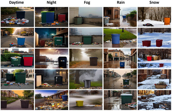
Figure 7.
Examples of images generated through the text-to-image process.
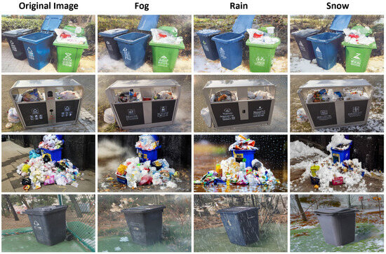
Figure 8.
Examples of images generated through the image-to-image process.
In our experiments, approximately half of the generated images exhibit various issues. In order to be consistent with authenticity in the real-world scenarios, we conducted a thorough screening and eliminated all problematic images. There are three main issues found in problematic images:
- Subject distortion: The garbage bins appear deformed, distorted, or blended with other objects (e.g., flower pots or lockers), making them difficult to recognize.
- Subject absence: The garbage bins in the image are either too small or entirely missing.
- Unrealistic appearance: The images exhibit overly fantastical or cartoonish styles or include phenomena that violate physical laws.
Figure 9 illustrates examples of problematic images from the three abovementioned categories. Each of the images that were ultimately removed exhibited at least one of these three issues. After the screening process, a total of 8408 images were successfully obtained.
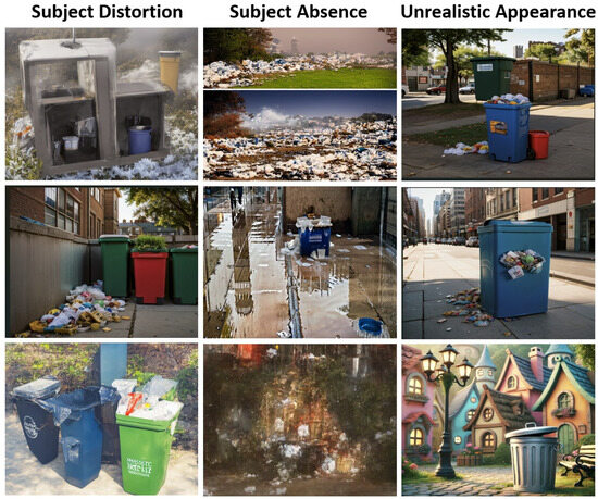
Figure 9.
Examples of problematic images.
In addition to rigorous manual screening, we evaluated the quality of images generated by the SD model using the Naturalness Image Quality Evaluator (NIQE) [41]. NIQE is a no-reference image quality assessment metric that evaluates image quality based on natural scene statistics, with lower values indicating higher quality. For reference, we also took 100 high-quality photos in various real-world scenarios. The experimental subjects consisted of two sets of images: the first set included 1000 randomly selected images from the web-scraped dataset that had not been enhanced with SD, and the second set included 1000 randomly selected images from the dataset that had been enhanced with SD after manual screening.
As shown in Table 2, the average NIQE value for the real-world photos was 3.5001, while the average NIQE value for the web-scraped photos was 4.4819. The average NIQE value for all generated images was 3.5548. These results indicate that, according to the NIQE evaluation, the dataset enhanced by the SD model and manually screened exhibits relatively high quality, closely approximating that of the real-world photos, and is significantly superior to the web-scraped photos.
Table 2.
Average NIQE values for different image sets.
3.1.5. Data Augmentation
Data augmentation is a technique to increase the size and diversity of the training dataset by applying various transformations and modifications to the original data, thereby improving the generalization ability of the model and reducing the risk of overfitting [42,43]. We primarily adopted three data augmentation methods: horizontal flipping, horizontal scaling and brightness adjustment. Figure 10 shows an image to which three augmentation methods were applied. As a result, horizontal flipping and horizontal scaling yielded 1673 and 1665 transformed images, respectively. Random brightness adjustment produced 1676 images. In total, these augmentation methods resulted in 5014 new images as detailed in the Table 3.
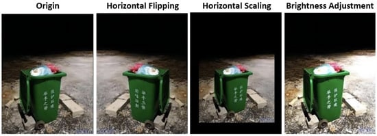
Figure 10.
An example of an image to which three augmentation methods were applied. (The Chinese characters on the garbage bin in the picture means, “A small effort protects the environment”).
Table 3.
Number of pictures transformed by data augmentation.
Following the generation process utilizing the SD model and subsequent data augmentation techniques, our dataset now comprises a total of 16,771 images. The distribution of labels within the GBS dataset is illustrated in Figure 11. This dataset offers an extensive and varied collection of images of garbage bins, enabling the robust training and evaluation of our proposed methods.
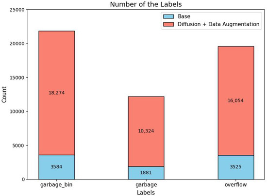
Figure 11.
The distribution of labels within the GBS dataset.
3.2. Proposed Garbage Bin Overflow Detection Model
3.2.1. Introduction to SNNs
SNNs are designed to mimic the behavior of biological neurons in the brain, with the goal of achieving more realistic and energy-efficient artificial intelligence. The human brain, renowned for its ability to perform complex cognitive tasks, operates on approximately 20 watts of energy. Although both artificial neural networks (ANNs) and SNNs draw inspiration from biological neural networks [44], ANNs have not fully adopted the energy-efficiency characteristics inherent to biological neurons. Structurally, the fundamental distinction between SNNs and ANNs is that SNN neurons employ models that mimic the behavior of biological neurons, and transmit information through discrete-time sequences of spikes [45]. The structures of SNN neurons and ANN neurons are shown in Figure 12. This feature enables SNNs to achieve energy-efficient functionality similar to biological neurons in two ways. First, SNNs operate on an event-driven basis: neurons spike only when their inputs exceed a set threshold, contrasting with ANNs that maintain continuous computation regardless of input levels. This feature, known as selective firing, can significantly reduce the computational load and energy consumption. Second, SNNs transmit information in the form of pulses. This mode of transmission significantly reduces computational complexity when compared to the continuous value operations carried out by ANNs during matrix computations. The energy efficiency of SNNs renders them particularly advantageous for applications on mobile devices. While SNNs offer significant advantages in energy efficiency, they also come with certain drawbacks compared to ANNs: First, training SNNs is more challenging due to the non-differentiable nature of spike-based computations. Second, for many tasks, SNNs still lag behind state-of-the-art ANNs in terms of accuracy, especially in large-scale and complex datasets [46]. However, SNNs are capable of leveraging spatiotemporal information effectively. By encoding and transmitting information via the temporal sequence of spikes, SNNs exhibit superior performance in processing dynamic data, such as video streams and sensor data. While there remain certain gaps in detection accuracy between SNNs and state-of-the-art ANNs for many scenes, the accuracy achieved by the SNN object detection algorithms is sufficient for the garbage bin overflow detection task undertaken in this study.
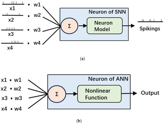
Figure 12.
The structures of SNN neurons (a) and ANN neurons (b).
One common neuron model used in SNNs is the Leaky Integrate-and-Fire (LIF) neuron model. In the LIF neuron model, each neuron integrates incoming spikes over time, with the leakage term that models the gradual decay of the neuron’s membrane potential in the absence of input. When the membrane potential reaches a certain threshold, the neuron fires the spike and resets its potential to the resting state. In its simplest form, the LIF neuron model can be expressed mathematically as the following differential equation:
where is the membrane potential of the neuron at time t, is the membrane time constant, is the resting potential of the neuron, is the membrane resistance, and is the input current to the neuron at time t. The following Algorithm 1 presents a pseudo-code implementation of the LIF model to facilitate the understanding of its workflow.
| Algorithm 1 Integrate-and-Fire neuron model simulation algorithm. | ||
| 1: | Parameters Initialization: | |
| 2: | ▹ Resting potential (e.g., −70 mV) | |
| 3: | ▹ Membrane time constant (ms) | |
| 4: | ▹ Membrane resistance | |
| 5: | ▹ Threshold potential (e.g., −55 mV) | |
| 6: | ▹ Reset potential (mV) | |
| 7: | ▹ Time step (ms) | |
| 8: | Initialize | ▹ Initial membrane potential |
| 9: | ||
| 10: | for each time step t do | |
| 11: | ▹ Input current from presynaptic neurons or stimuli | |
| 12: | ||
| 13: | ||
| 14: | if then | |
| 15: | emit_spike() | ▹ Emit a spike |
| 16: | ▹ Reset the membrane potential | |
| 17: | end if | |
| 18: | end for | |
3.2.2. Energy Consumption of SNNs and ANNs
The energy consumption of running SNNs on neuromorphic hardware is often assessed using the performed number of operations. In ANNs, each operation typically involves the multiplication and addition of floating-point numbers, referred to as multiply–accumulate (MAC) operations. The MAC operations perform a multiply–accumulate function, involving multiplication followed by addition and storage of the outcome [47].
In SNNs, energy efficiency is optimized by ensuring that neurons only participate in Accumulation Calculations (ACs) upon spiking. This process involves a processor sequentially summing a series of numerical values and then storing the result. ACs consume less energy than MAC operations [48]. By taking into account the energy consumption of both MAC operations and ACs, the formula for calculating network energy consumption can be defined as
where and represent the average energy consumed per AC and MAC operation. and are the total numbers of MAC operations and ACs. T and represent the number of time steps and the firing rate of a single block. n stands for the nth block.
3.2.3. HERD-YOLO
The proposed model in this study builds on the architecture of the Energy-efficient Membrane-Shortcut-YOLO (EMS-YOLO) model [49]. EMS-YOLO is a deep SNN model designed for object detection, currently recognized as one of the best-performing models in the domain of SNN-based object detection. EMS-YOLO generally follows the architecture of YOLOv3 [50], integrating the ResNet [51] architecture and predicting detection boxes at two different scales. The backbone of EMS-YOLO is primarily constituted by the Energy-efficient Membrane-Shortcut Res Block (EMS-Block) and its variants, including MS-Block, EMS-Block1, and EMS-Block2. The EMS-block is developed by converting a Res Block from the ANN architecture to the SNN architecture, with refinements made to the finer details. Each variant plays a unique role within the EMS-ResNet architecture, enhancing the overall efficiency and performance of the network. The key structure of EMS-Block is illustrated in Figure 13a.
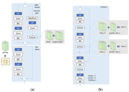
Figure 13.
The structure of EMS-Block (a) and the proposed ED-Block (b).
To more effectively address the challenge of detecting overflowing garbage bins, we introduced the Energy-Efficient Dense Block (ED-Block) as a feature extraction module in the backbone of our detection model. The key structure of the ED-Block is presented in Figure 13b. The ED-Block was derived from the Dense Block [30] through the conversion process from the ANN architecture to the SNN architecture. Some targeted refinements were made to improve its performance as well. A Dense block can be represented by
where represents the non-linear activation function of layer i, while signifies the output of layer i. The notation denotes the concatenation of the output feature maps from layer 0 to layer . Furthermore, for all , the dimension of is determined by the hyperparameter referred to as the growth rate.
The ED-Block was featured with dense connections, which significantly increases the parameter sharing rate. The network constructed with ED-Blocks achieved a reduction in the total number of parameters and a consequent decrease in the computational requirements. These benefits are particularly well suited to the lightweight and energy-efficient demands of garbage bin overflow detection tasks. Furthermore, our approach stands out also due to the inclusion of a pre-spike structure within the proposed ED-Block, drawing inspiration from Ho et al. [20]. Unlike previous methods, our ED-Block introduced LIF units prior to each convolutional operation. The spikes generated by these LIF units were directly input into the convolutional layers for normalization. Subsequently, these normalized spikes accumulated into membrane potentials, which were then passed on to the subsequent layer of LIF units.
Based on the ED-Block, we constructed the deep SNN object detection network: Hybrid Energy-Efficient ResDense YOLO (HERD-YOLO). HERD-YOLO integrates both EMS-Block and ED-Block within the YOLO framework. As illustrated in Figure 14, within the Herd-YOLO network, the LCB block serves as the most crucial fundamental unit. The LCB, which comprises Leaky LIF neurons, convolutional layers, and Batch Normalization (BN) layers, operates as follows: At each time step, it receives input spike signals to activate the neurons, performs convolution on the output spikes of each neuron, normalizes the results, and subsequently passes them to the next unit. Likewise, the workflow of the entire SNN follows a similar pattern: For each input sample, the input signal is first converted into a spike sequence. At each time step, for each neuron, the LIF neuron model update is performed. If a neuron generates a spike, the input to downstream neurons is updated accordingly. Ultimately, the final spike sequence or decoded result is produced as the output.
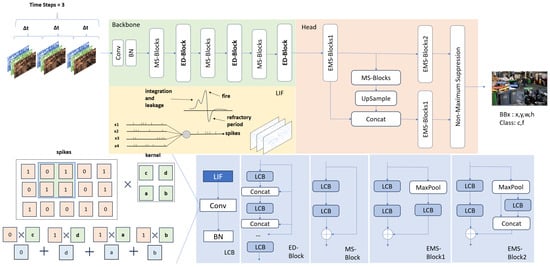
Figure 14.
The structure of Hybrid Energy-Efficient ResDense YOLO (HERD-YOLO).
HERD-YOLO primarily comprised a backbone network and a detection head. The backbone network employed multiple ED-Blocks and MS-Blocks to extract object features across different dimensions and channel quantities. Specifically, three ED-Blocks were utilized, characterized by 4, 8, and 16 convolutional layers, respectively. Each of these layers was configured with the stride of 1, the kernel size of 3, and the padding of 1. The ED-Blocks were designed to progressively increase the channel count of feature maps, maintaining a fixed growth rate of 16. After each ED-Block, a convolutional layer with a stride of 2 was applied to reduce the computational complexity by downsizing the feature maps. Between each ED-Block, MS-Blocks were integrated to deepen the network, thereby enhancing the learning capability of the model and alleviating issues related to gradient vanishing and gradient explosion.
For the detection head, HERD-YOLO directly adopted the same architecture as EMS-YOLO. The detection head was designed to prevent the performance degradation often encountered in SNNs, which was due to the multi-layer, direct-connected convolution structure present in traditional detection heads [49]. The central challenge for the detection head of HERD-YOLO is the conversion of spike information into accurate continuous value representations for bounding box coordinates. To tackle this, we utilized the last membrane potential of the neurons as input, which was then fed into each detector to produce anchors of various sizes. Following the application of Non-Maximum Suppression (NMS), we obtained the definitive categories, bounding box coordinates, and confidence scores for different objects.
4. Results and Discussion
4.1. Model Validation Experiment
To comprehensively evaluate the performance of our model in detecting the overflow of garbage bins, we conducted a comparative analysis of the proposed HERD-YOLO and EMS-YOLO models using PyTorch (1.7.0) with the GBS dataset. PyTorch is an open-source machine learning library based on the Python programming language, used for applications such as computer vision and natural language processing. For these experiments, a single 10 GB Nvidia GeForce RTX 3080 graphics card was utilized. The GBS dataset was partitioned into training, validation, and test sets in a proportion of 7:1:2. Specifically, the training set comprised 11,740 images, the validation set contained 1677 images, and the test set consisted of 3354 images. For HERD-YOLO, the Stochastic Gradient Descent (SGD) optimizer was employed, with a learning rate set at 0.01. The loss function consists of three components: bounding box regression loss, object confidence loss, and classification loss. Specifically, the bounding box regression loss was determined using Generalized Intersection over Union (GIoU). Both the object confidence loss and the classification loss were calculated using function BCEWithLogitsLoss. Finally, these three components were weighted and combined to yield the total loss. The images in the GBS dataset have all been resized to 640 × 640 pixels for model training. All models were trained on the training set for a total of 300 epochs, with each batch consisting of 16 samples. Following the training process, unified test results were generated based on the test set.
Since the most prominent advantage of the SNNs lies in its energy efficiency, a comparison of the energy consumption of HERD-YOLO under the ANN and SNN architectures was conducted using Equation (2). It was assumed that all computations were performed using a 32-bit floating-point format, employing 45 nm technology. Therefore, pJ and pJ were set, respectively. The membrane time constant was set to 0.25. The resting potential for LIF neurons was maintained at 0.25, and the threshold for the action potential of LIF neurons was established at 0.5.
The comparative experiments were conducted to evaluate the HERD-YOLO and EMS-YOLO models across two distinct neural network architectures: ANNs and SNNs. Table 4 shows the detailed results, which were obtained from well-trained models evaluated on test sets. Within Table 4, we present the number of parameters, time step (specific to SNNs), mAP@0.5, mAP@0.5:0.95, firing rate (specific to SNNs), and energy cost for the HERD-YOLO and EMS-YOLO models under both ANN and SNN architectures, respectively. mAP@0.5 is the Mean Average Precision at Intersection over Union (IoU) threshold of 0.5, which measures the average precision of a detection model across all classes when the IoU threshold for considering a detection as correct is set to 0.5. Similarly, mAP@0.5:0.95 is the Mean Average Precision at IoU thresholds from 0.5 to 0.95. This is a more rigorous evaluation that calculates the average precision at each IoU threshold between 0.5 and 0.95, providing a comprehensive assessment of a model’s ability to detect objects across varying levels of strictness in overlap criteria. It is observed that both models possess comparable parameter sizes, with EMS-YOLO having 25.27 million parameters and HERD-YOLO being slightly smaller with 24.76 million parameters. This similarity in parameter sizes remains constant in both the ANN and SNN architectures, thus ensuring a fair comparison for performance between the two models.
Table 4.
The performance of the HERD-YOLO and EMS-YOLO models across their ANNs and SNNs versions on the GBS dataset.
The detection accuracy of both models was evaluated by the mAP@0.5 and mAP@0.5:0.95 metrics. Under the mAP@0.5 metric, HERD-YOLO achieves a higher precision with scores of 0.954 under the ANN architecture and 0.953 under the SNN architecture, compared to EMS-YOLO’s respective values of 0.950 and 0.948. The same results of both models under the SNN architecture are also present in the PR curves in Figure 15. The advantage of HERD-YOLO becomes even more evident under the more rigorous mAP@0.5:0.95 metric, where it outperforms EMS-YOLO under both the ANN and SNN architectures as well. The above two metrics highlight the superior capability of HERD-YOLO across all classes to handle a broader spectrum of IoU thresholds, indicating its improved performance across a variety of detection criteria.
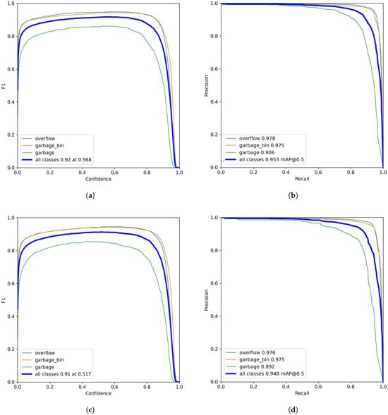
Figure 15.
The F1–Confidence and PR curves of HERD-YOLO and EMS-YOLO. (a) F1–Confidence curve of HERD-YOLO. (b) PR curve of HERD-YOLO. (c) F1–Confidence curve of EMS-YOLO. (d) PR curve of EMS-YOLO.
HERD-YOLO distinguishes itself by its reduced energy consumption and lower firing rate. HERD-YOLO has a firing rate of 16.17%, which is more efficient than EMS-YOLO with a firing rate of 18.36%, indicating its superior spike-based computation capabilities. Note that we have normalized the energy consumption of EMS-YOLO under the ANN architecture to the baseline value of 1, with all other values in the row being proportional to this standard.
The SNN architecture clearly shows lower energy consumption than the ANN architecture, reducing energy use to about one-tenth. Specifically, HERD-YOLO achieves a significant reduction in energy consumption, decreasing it by 27.0% compared to EMS-YOLO and by 89.2% compared to the corresponding model under the ANN architecture. These results suggest that HERD-YOLO is a more energy-efficient model, making it particularly well suited for resource-limited environments such as edge devices.
Figure 15 presents the F1–Confidence and Precision–Recall (PR) curves for HERD-YOLO and EMS-YOLO. The comparative analysis spans three classes: overflowing garbage bins, non-overflowing garbage bins, and garbage, labeled as “overflow”, “garbage_bin”, and “garbage”, respectively. The F1–Confidence curve of HERD-YOLO indicates a high F1 score across various confidence levels, peaking at 0.92 for all classes at a confidence level of 0.568. In contrast, EMS-YOLO has a lower peak F1 score of 0.91 at a lower confidence level of 0.517. This result suggests that HERD-YOLO is more adept at accurately identifying positive instances while maintaining a high level of precision, even when the prediction threshold is set higher. In the PR curves, HERD-YOLO also demonstrates superior performance in terms of precision, especially in the “garbage” class, where it achieves a precision of 0.906 compared to 0.892 of EMS-YOLO. Under the mAP@0.5, the overall precision of HERD-YOLO across all classes is 0.953, outperforming EMS-YOLO’s precision of 0.948. This result is consistent with Table 4. However, the F1 curve and precision for the “garbage” class in HERD-YOLO are much lower than those for the other two classes. This discrepancy is likely due to the relatively fewer labeled instances available for the “garbage” class compared to the other two classes.
4.2. Validation of Data Augmentation Strategies
To verify the effectiveness of our data augmentation, we employed 3349 web-scraped images from our base dataset as the baseline training dataset and the GBS dataset as the experimental dataset. The web-scraped images predominantly depicted garbage bins in ideal lighting and clear weather conditions, whereas the GBS dataset encompassed scenarios of garbage bins in a variety of complex environments. The HERD-YOLO model was employed for training, and the training process was conducted using the same settings as those in the model validation experiment. The detection performance of the models trained on these two distinct datasets was subsequently evaluated on a test set comprising 110 images. The test set used here was additionally sourced from online downloads and field photography, and was not included in the GBS dataset. Furthermore, to validate the model’s generalization ability, the test set was designed to include scenarios of garbage bins under diverse lighting and weather conditions. Table 5 presents the detailed results, which clearly demonstrate that the HERD-YOLO model trained on the GBS dataset significantly outperforms the model trained solely on the web-scraped dataset when evaluated on the designed test set. This underscores the efficacy of our data augmentation strategy.
Table 5.
Performance comparison of HERD-YOLO on different training datasets.
To further corroborate the enhanced detection capability of the model trained on the GBS dataset in complex environments, several representative detection results that highlight the performance gap were selected. As illustrated in Figure 16a, the model trained on the GBS dataset accurately detects two overflowing garbage bins in a dark environment. Figure 16b depicts two garbage bins in a snowy setting, where the model trained on the GBS dataset successfully identifies both bins despite the interference of snow cover. In Figure 16c, the model trained on the GBS dataset not only correctly localizes the overflowing garbage bin and the scattered garbage but also achieves this with higher confidence scores. Collectively, these results underscore the efficacy of the GBS dataset in augmenting the model’s detection generalization across diverse and challenging scenarios.
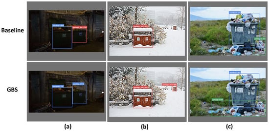
Figure 16.
Comparison of selected detection results. (a) illustrates two overflowing garbage bins in a dark environment, (b) depicts two garbage bins covered in snow, (c) displays waste and overflowing garbage bins in daytime within an overgrown grassland.
In conclusion, HERD-YOLO consistently demonstrates superior performance over EMS-YOLO under both ANN and SNN architectures. It achieves higher detection precision while significantly reducing energy consumption. Furthermore, the validation of data augmentation strategies has confirmed the generalization ability of HERD-YOLO. These improvements suggest that HERD-YOLO is a more efficient and robust model for the task of detecting overflowing garbage bins.
5. Conclusions and Future Work
Employing intelligent detection systems to monitor the overflow status of garbage bins in real-time has emerged as a crucial approach in efficient waste management. This study addressed two key issues in garbage bin overflow detection. Firstly, we developed the GBS dataset for garbage bin overflow detection, which consists of 16,771 images in total. The dataset is partitioned into three distinct subsets: the base dataset (3349 images), the generated dataset (8408 images), and the augmented dataset (5014 images). The generated dataset was created using the SD model through two distinct generation processes: text-to-image and image-to-image generation. By leveraging the SD model, we successfully generated images of garbage bins under a variety of environmental conditions. This approach significantly enhances the generalization capability of the detection model integrated into intelligent garbage bin detection systems, allowing the model to operate more effectively in complex and variable real-world environments. Furthermore, the GBS dataset will also support other related research.
Secondly, we developed HERD-YOLO, a garbage bin overflow detection model that utilized SNNs and was trained with our GBS dataset. HERD-YOLO achieved an mAP@0.5 of 0.953. Additionally, it significantly reduced energy consumption by 89.2% compared to the corresponding model under the ANN architecture, and by 27.0% compared to EMS-YOLO. The combination of high detection accuracy and low energy consumption makes HERD-YOLO a highly valuable solution for deployment on IoT devices. Our efforts in exploring and optimizing these two aspects have led to an enhancement in the efficiency of garbage bin overflow detection algorithms.
Future work will center on the following aspects to improve the robustness and scalability of intelligent detection systems in waste management. First, we will maintain a continuous effort to update and expand the GBS dataset with a wider variety of images, thereby improving the generalization capabilities of the model. Second, we will refine strategies for deploying the HERD-YOLO model on various IoT devices, aiming to maximize its practicality in real-world scenarios. Third, we will explore the application of more advanced neural network architectures and training techniques, including transfer learning and federated learning, in order to further elevate model performance. By addressing these areas, we aim to not only improve the waste management process, making it more efficient and intelligent, but also reduce labor costs, thus contributing to the sustainable development of the urban environment.
Author Contributions
Conceptualization, C.M.; methodology, L.Y.; software, L.Y. and X.Z.; validation, L.Y. and X.Z.; investigation, J.H.; resources, C.M.; data curation, L.Y., X.Z., J.H., Z.L. and J.C.; writing—original draft preparation, L.Y.; writing—review and editing, C.M.; visualization, L.Y. and X.Z.; supervision, C.M.; project administration, C.M.; funding acquisition, C.M. All authors have read and agreed to the published version of the manuscript.
Funding
This research is supported by the Natural Science Foundation of Shandong Province, China (Grant No. 1090413702304).
Institutional Review Board Statement
Not applicable.
Informed Consent Statement
Not applicable.
Data Availability Statement
The code used in this study was shared in GitHub repository at https://github.com/Rah-xephon/HERD-Yolo, accessed on 18 April 2025. The GBS dataset was share online at https://zenodo.org/records/14711706, accessed on 18 April 2025.
Acknowledgments
This work is supported by the Natural Science Foundation of Shandong Province, China (Grant No. 1090413702304). The authors would like to thank Liang Guo for contributing to this work.
Conflicts of Interest
The authors declare no conflicts of interest.
References
- Catania, V.; Ventura, D. An Approch for Monitoring and Smart Planning of Urban Solid Waste Management Using Smart-M3 Platform. In Proceedings of the 15th Conference of Open Innovations Association FRUCT, St. Petersburg, Russia, 21–25 April 2014; pp. 24–31. [Google Scholar] [CrossRef]
- Abba, S.; Light, C.I. IoT-Based Framework for Smart Waste Monitoring and Control System: A Case Study for Smart Cities. Eng. Proc. 2020, 2, 90. [Google Scholar] [CrossRef]
- Birara, E.; Kassahun, T. Assessment of solid waste management practices in Bahir Dar City, Ethiopia. Pollution 2018, 4, 251–261. [Google Scholar]
- Derhab, N.; Elkhwesky, Z. A systematic and critical review of waste management in micro, small and medium-sized enterprises: Future directions for theory and practice. Environ. Sci. Pollut. Res. 2023, 30, 13920–13944. [Google Scholar] [CrossRef]
- Ram, M.; Bracci, E. Waste Management, Waste Indicators and the Relationship with Sustainable Development Goals (SDGs): A Systematic Literature Review. Sustainability 2024, 16, 8486. [Google Scholar] [CrossRef]
- Lokhande, P.; Pawar, M. A review: Garbage collection management system. Int. J. Res. Eng. Technol. 2016, 5, 79–82. [Google Scholar]
- Fauziah; Bakri, I. Esthetic, integrated, smart and green trash bin for public space: A review. IOP Conf. Ser. Earth Environ. Sci. 2020, 575, 012240. [Google Scholar] [CrossRef]
- Joshi, A.; Deshmukh, A.; Auti, A. The Future of Smart Waste Management in Urban Areas: A Holistic Review. In Proceedings of the 2023 International Conference on Next Generation Electronics (NEleX), Vellore, India, 14–16 December 2023; pp. 1–6. [Google Scholar] [CrossRef]
- Sohag, M.U.; Podder, A.K. Smart garbage management system for a sustainable urban life: An IoT based application. Internet Things 2020, 11, 100255. [Google Scholar] [CrossRef]
- Sosunova, I.; Porras, J. IoT-Enabled Smart Waste Management Systems for Smart Cities: A Systematic Review. IEEE Access 2022, 10, 73326–73363. [Google Scholar] [CrossRef]
- Wang, Y.; Zheng, H.; Mao, C.; Zhang, J.; Ke, X. Deep Learning-based Multi-task Network for Intelligent Management of Garbage Deposit Points. In Proceedings of the 2021 11th International Conference on Information Technology in Medicine and Education (ITME), Wuyishan, China, 19–21 November 2021; pp. 251–256. [Google Scholar] [CrossRef]
- Wahyutama, A.B.; Hwang, M. YOLO-Based Object Detection for Separate Collection of Recyclables and Capacity Monitoring of Trash Bins. Electronics 2022, 11, 1323. [Google Scholar] [CrossRef]
- Wang, Y.; Muthu, B.; Anbarasan, M. Research on Intelligent Trash Can Garbage Classification Scheme Based on Improved YOLOv3 Target Detection Algorithm. J. Interconnect. Networks 2022, 22, 2144004. [Google Scholar] [CrossRef]
- Sharma, R.K.; Mogha, N.; Saini, M.; Kumar, A. Garbage Bin Status Indicator Based on Multilayer Convolutional Neural Networks. 2023. Available online: https://colab.ws/articles/10.2139%2Fssrn.4489022 (accessed on 20 May 2024).
- Oğuz, A.; Ertuğrul, Ö.F. Determining the fullness of garbage containers by deep learning. Expert Syst. Appl. 2023, 217, 119544. [Google Scholar] [CrossRef]
- Ramson, S.R.J.; Moni, D.J.; Vishnu, S.; Anagnostopoulos, T.; Kirubaraj, A.A.; Fan, X. An IoT-based bin level monitoring system for solid waste management. J. Mater. Cycles Waste Manag. 2021, 23, 516–525. [Google Scholar] [CrossRef]
- Arthur, M.P.; Shoba, S.; Pandey, A. A survey of smart dustbin systems using the IoT and deep learning. Artif. Intell. Rev. 2024, 57, 56. [Google Scholar] [CrossRef]
- Su, H.; Gao, H.; Wang, X.; Fang, X.; Liu, Q.; Huang, G.; Li, X.; Cao, Q. Object Detection in Adverse Weather for Autonomous Vehicles Based on Sensor Fusion and Incremental Learning. IEEE Trans. Instrum. Meas. 2024, 73, 2535510. [Google Scholar] [CrossRef]
- Kumari, S.; Srivastava, M. An Energy Efficient System for IoT Enabled Smart Applications: Research Challenges and Open Issues. In Proceedings of the 2023 Seventh International Conference on Image Information Processing (ICIIP), Solan, India, 22–24 November 2023; pp. 570–575. [Google Scholar] [CrossRef]
- Ho, J.; Jain, A.; Abbeel, P. Denoising Diffusion Probabilistic Models. arXiv 2020, arXiv:2006.11239. [Google Scholar] [CrossRef]
- Kaur, P.; Khehra, B.S.; Mavi, E.B.S. Data Augmentation for Object Detection: A Review. In Proceedings of the 2021 IEEE International Midwest Symposium on Circuits and Systems (MWSCAS), Lansing, MI, USA, 9–11 August 2021; pp. 537–543. [Google Scholar] [CrossRef]
- Cao, Z.; Hidalgo Martinez, G.; Simon, T.; Wei, S.; Sheikh, Y.A. OpenPose: Realtime Multi-Person 2D Pose Estimation using Part Affinity Fields. IEEE Trans. Pattern Anal. Mach. Intell. 2019, 43, 172–186. [Google Scholar] [CrossRef]
- Wojke, N.; Bewley, A.; Paulus, D. Simple Online and Realtime Tracking with a Deep Association Metric. In Proceedings of the 2017 24th IEEE International Conference on Image Processing (ICIP), Beijing, China, 17–20 September 2017; pp. 3645–3649. [Google Scholar]
- Deng, J.; Guo, J.; Niannan, X.; Zafeiriou, S. ArcFace: Additive Angular Margin Loss for Deep Face Recognition. In Proceedings of the CVPR, Long Beach, CA, USA, 15–20 June 2019. [Google Scholar]
- Ramalingam, B.; Hayat, A.A.; Elara, M.R.; Félix Gómez, B.; Yi, L.; Pathmakumar, T.; Rayguru, M.M.; Subramanian, S. Deep Learning Based Pavement Inspection Using Self-Reconfigurable Robot. Sensors 2021, 21, 2595. [Google Scholar] [CrossRef]
- Gómez, B.F.; Yi, L.; Ramalingam, B.; Rayguru, M.M.; Hayat, A.A.; Thejus, P.; Leong, K.; Elara, M.R. Deep Learning based Litter Identification and Adaptive Cleaning using Self-reconfigurable Pavement Sweeping Robot. In Proceedings of the 2022 IEEE 18th International Conference on Automation Science and Engineering (CASE), Mexico City, Mexico, 20–24 August 2022; pp. 2301–2306. [Google Scholar] [CrossRef]
- Badrinarayanan, V.; Kendall, A.; Cipolla, R. SegNet: A Deep Convolutional Encoder-Decoder Architecture for Image Segmentation. IEEE Trans. Pattern Anal. Mach. Intell. 2017, 39, 2481–2495. [Google Scholar] [CrossRef]
- LeCun, Y.; Boser, B.; Denker, J.; Henderson, D.; Howard, R.; Hubbard, W.; Jackel, L. Handwritten Digit Recognition with a Back-Propagation Network. In Advances in Neural Information Processing Systems; Morgan-Kaufmann: San Francisco, CA, USA, 1989; Volume 2. [Google Scholar]
- Laguna, R. Clean Dirty Containers in Montevideo. Available online: https://www.kaggle.com/rodrigolaguna/clean-dirty-containers-in-montevideo (accessed on 16 April 2025).
- Huang, G.; Liu, Z.; Van Der Maaten, L.; Weinberger, K.Q. Densely Connected Convolutional Networks. In Proceedings of the 2017 IEEE Conference on Computer Vision and Pattern Recognition (CVPR), Honolulu, HI, USA, 21–26 July 2017; pp. 2261–2269. [Google Scholar] [CrossRef]
- Tan, M.; Le, Q. EfficientNet: Rethinking Model Scaling for Convolutional Neural Networks. In Proceedings of the 36th International Conference on Machine Learning, Long Beach, CA, USA, 9–15 June 2019; Volume 97, pp. 6105–6114. [Google Scholar]
- Howard, A.; Sandler, M.; Chu, G.; Chen, L.C.; Chen, B.; Tan, M.; Wang, W.; Zhu, Y.; Pang, R.; Vasudevan, V.; et al. Searching for MobileNetV3. In Proceedings of the 2019 IEEE/CVF International Conference on Computer Vision (ICCV 2019), Seoul, Republic of Korea, 27 October–2 November 2019; pp. 1314–1324. [Google Scholar] [CrossRef]
- Simonyan, K.; Zisserman, A. Very Deep Convolutional Networks for Large-Scale Image Recognition. arXiv 2014, arXiv:1409.1556. [Google Scholar] [CrossRef]
- Kausar, M.A.; Dhaka, V.; Singh, S.K.; de Kunder, M. Web Crawler: A Review. Int. J. Comput. Appl. 2013, 63, 31–36. [Google Scholar] [CrossRef]
- Thabtah, F.; Hammoud, S.; Kamalov, F.; Gonsalves, A. Data imbalance in classification: Experimental evaluation. Inf. Sci. 2020, 513, 429–441. [Google Scholar] [CrossRef]
- Rombach, R.; Blattmann, A.; Lorenz, D.; Esser, P.; Ommer, B. High-Resolution Image Synthesis With Latent Diffusion Models. In Proceedings of the Proceedings of the IEEE/CVF Conference on Computer Vision and Pattern Recognition (CVPR), New Orleans, LA, USA, 18–24 June 2022; pp. 10684–10695. [Google Scholar] [CrossRef]
- Kingma, D.P.; Welling, M. Auto-Encoding Variational Bayes. arXiv 2013, arXiv:1312.6114. [Google Scholar] [CrossRef]
- Radford, A.; Kim, J.W.; Hallacy, C.; Ramesh, A.; Goh, G.; Agarwal, S.; Sastry, G.; Askell, A.; Mishkin, P.; Clark, J.; et al. Learning Transferable Visual Models From Natural Language Supervision. In Proceedings of the 38th International Conference on Machine Learning, Virtual Event, 18–24 July 2021; Volume 139, pp. 8748–8763. [Google Scholar]
- Karras, T.; Aittala, M.; Aila, T.; Laine, S. Elucidating the Design Space of Diffusion-Based Generative Models. arXiv 2022, arXiv:2206.00364. [Google Scholar] [CrossRef]
- Lu, C.; Zhou, Y.; Bao, F.; Chen, J.; Li, C.; Zhu, J. DPM-Solver++: Fast Solver for Guided Sampling of Diffusion Probabilistic Models. arXiv 2023, arXiv:2211.01095. [Google Scholar] [CrossRef]
- Mittal, A.; Soundararajan, R.; Bovik, A.C. Making a “Completely Blind” Image Quality Analyzer. IEEE Signal Process. Lett. 2013, 20, 209–212. [Google Scholar] [CrossRef]
- Perez, L.; Wang, J. The Effectiveness of Data Augmentation in Image Classification using Deep Learning. arXiv 2017, arXiv:1712.04621. [Google Scholar] [CrossRef]
- Shorten, C.; Khoshgoftaar, T.M. A survey on Image Data Augmentation for Deep Learning. J. Big Data 2019, 6, 60. [Google Scholar] [CrossRef]
- Wu, Y.C.; Feng, J.W. Development and Application of Artificial Neural Network. Wirel. Pers. Commun. 2018, 102, 1645–1656. [Google Scholar] [CrossRef]
- Maass, W. Networks of spiking neurons: The third generation of neural network models. Neural Netw. 1997, 10, 1659–1671. [Google Scholar] [CrossRef]
- Malcolm, K.; Casco-Rodriguez, J. A Comprehensive Review of Spiking Neural Networks: Interpretation, Optimization, Efficiency, and Best Practices. arXiv 2023, arXiv:2303.10780. [Google Scholar] [CrossRef]
- Sai Kumar, M.; Kumar, D.A.; Samundiswary, P. Design and performance analysis of Multiply-Accumulate (MAC) unit. In Proceedings of the 2014 International Conference on Circuits, Power and Computing Technologies [ICCPCT-2014], Nagercoil, India, 20–21 March 2014; pp. 1084–1089. [Google Scholar] [CrossRef]
- Horowitz, M. 1.1 Computing’s energy problem (and what we can do about it). In Proceedings of the 2014 IEEE International Solid-State Circuits Conference Digest of Technical Papers (ISSCC), San Francisco, CA, USA, 9–13 February 2014; pp. 10–14. [Google Scholar] [CrossRef]
- Su, Q.; Chou, Y.; Hu, Y.; Li, J.; Mei, S.; Zhang, Z.; Li, G. Deep directly-trained spiking neural networks for object detection. In Proceedings of the IEEE/CVF International Conference on Computer Vision, Paris, France, 1–6 October 2023; pp. 6555–6565. [Google Scholar]
- Redmon, J.; Farhadi, A. YOLOv3: An Incremental Improvement. arXiv 2018, arXiv:1804.02767. [Google Scholar] [CrossRef]
- He, K.; Zhang, X.; Ren, S.; Sun, J. Deep Residual Learning for Image Recognition. In Proceedings of the 2016 IEEE Conference on Computer Vision and Pattern Recognition (CVPR), Las Vegas, NV, USA, 27–30 June 2016; pp. 770–778. [Google Scholar] [CrossRef]
Disclaimer/Publisher’s Note: The statements, opinions and data contained in all publications are solely those of the individual author(s) and contributor(s) and not of MDPI and/or the editor(s). MDPI and/or the editor(s) disclaim responsibility for any injury to people or property resulting from any ideas, methods, instructions or products referred to in the content. |
© 2025 by the authors. Licensee MDPI, Basel, Switzerland. This article is an open access article distributed under the terms and conditions of the Creative Commons Attribution (CC BY) license (https://creativecommons.org/licenses/by/4.0/).