
Integrated Energy Management in Small-Scale Smart Grids Considering the Emergency Load Conditions: A Combined Battery Energy Storage, Solar PV, and Power-to-Hydrogen System

 , ,
, ,  and
and 
Abstract
Highlights
- Proposed a comprehensive modeling layout for the optimal management of power and heat in the distribution system, taking into account load emergencies such as overload and load shedding.
- Incorporated different energy sources, such as renewables, batteries, power to hydrogen, CHP sources, and heat storage tanks, as well as demand response programs for both electrical and thermal loads.
- The proposed approach aims to effectively balance the energy supply and demand in the network, especially during emergency situations, to certify the system’s reliability and stability.
- Provided a cost-effective and environmentally friendly solution for managing the distribution network, while also improving its resilience and reducing the risk of energy supply disruptions.
Abstract
1. Introduction
1.1. Literature
1.2. Motivation
1.3. Main Contribution
- −
- Comprehensive Multi-Source Integration: The model combines RERs (solar and wind), ESSs, CHP units, and P2H systems within a unified optimization framework, addressing both electrical and thermal energy demands. This integration strengthens the resilience and adaptability of small-scale SGs, ensuring reliable energy management across variable conditions.
- −
- Emergency Load Management: This study uniquely addresses emergency load conditions, such as load shedding and overload. Unlike traditional approaches that focus on standard operations, this model dynamically balances supply and demand during emergencies, improving grid stability and reducing the impact of sudden demand surges or supply disruptions.
- −
- Enhanced Flexibility through P2H Systems: Incorporating P2H systems allows excess electrical energy to be converted to hydrogen, expanding the feasible solution space for thermal and electrical loads. This flexibility benefits both resilience and sustainability by utilizing excess RE for thermal needs, reducing waste, and supporting a cleaner energy mix.
- −
- Dual DRPs: The model advances DRPs by applying them to both electrical and thermal loads. This dual approach maximizes demand-side flexibility, reducing the need for load shedding in high-demand situations and minimizing the dependency on emergency interventions, thus enhancing cost-effectiveness and operational efficiency.
- −
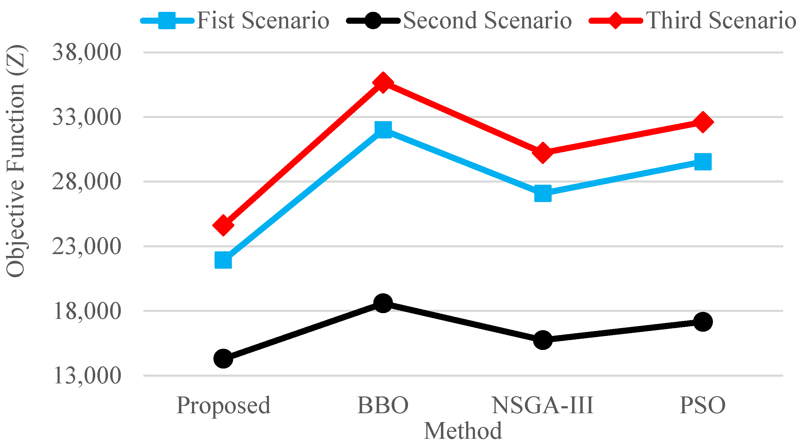
- Improved Computational Efficiency and Solution Optimality: Employing the Gurobi solver enables the model to achieve global optimality, surpassing traditional non-linear methods in efficiency and solution quality. In comparative tests, the model consistently outperformed algorithms like BBO, PSO, and NSGA-III, achieving better cost savings, emission reductions, and ELM.
- −
- Simulation of Practical Scenarios: This study examines three practical scenarios—normal operation, load shedding, and overload—demonstrating the model’s applicability to real-world conditions. By simulating diverse operational environments, the model proves highly adaptable and relevant to real-world SG applications.
1.4. Paper Structure
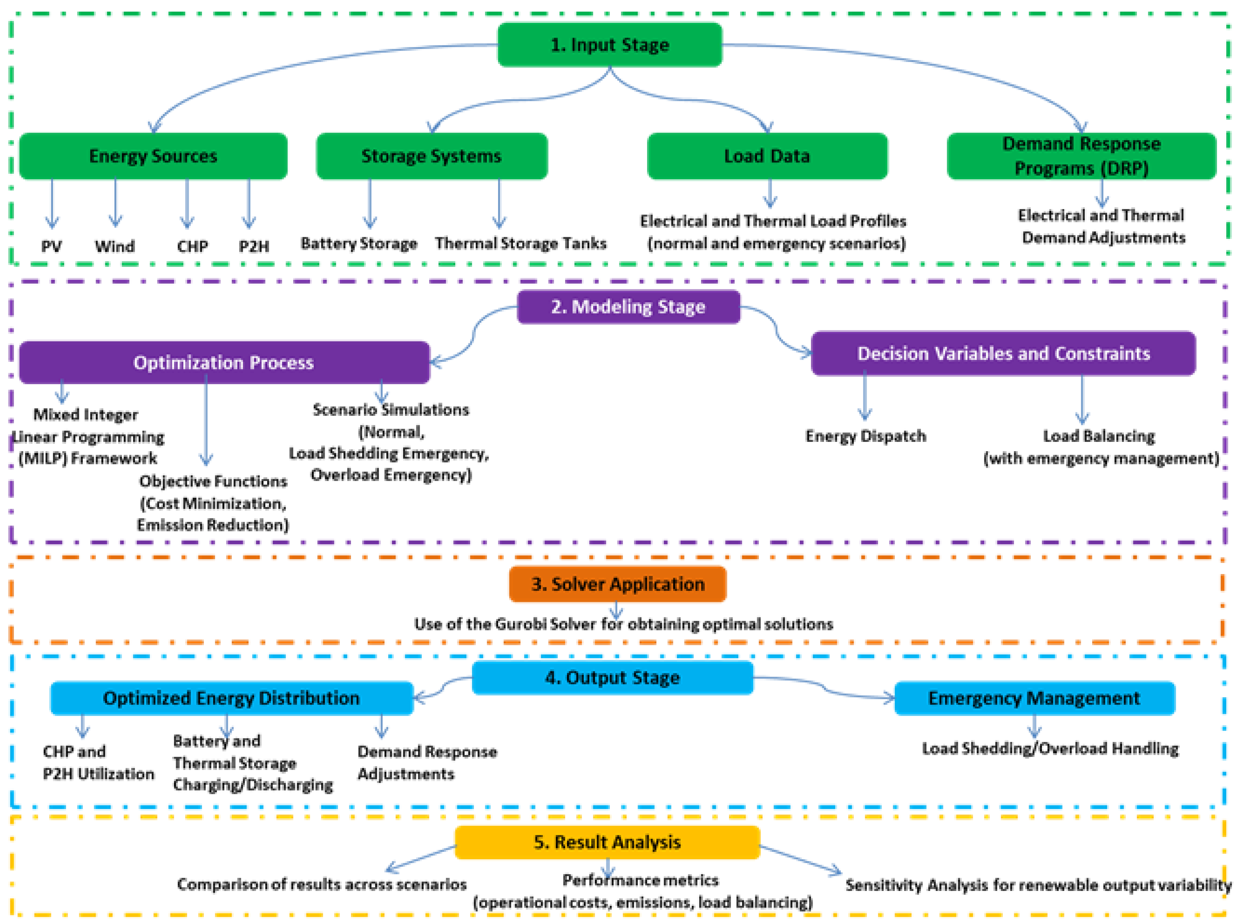
2. Proposed Energy Management Model
Proposed System and Solution Structure
3. Simulation Results
3.1. Data Preprocessing and Assumptions
3.1.1. Data Preprocessing
- (a)
- Energy Demand Data
- (b)
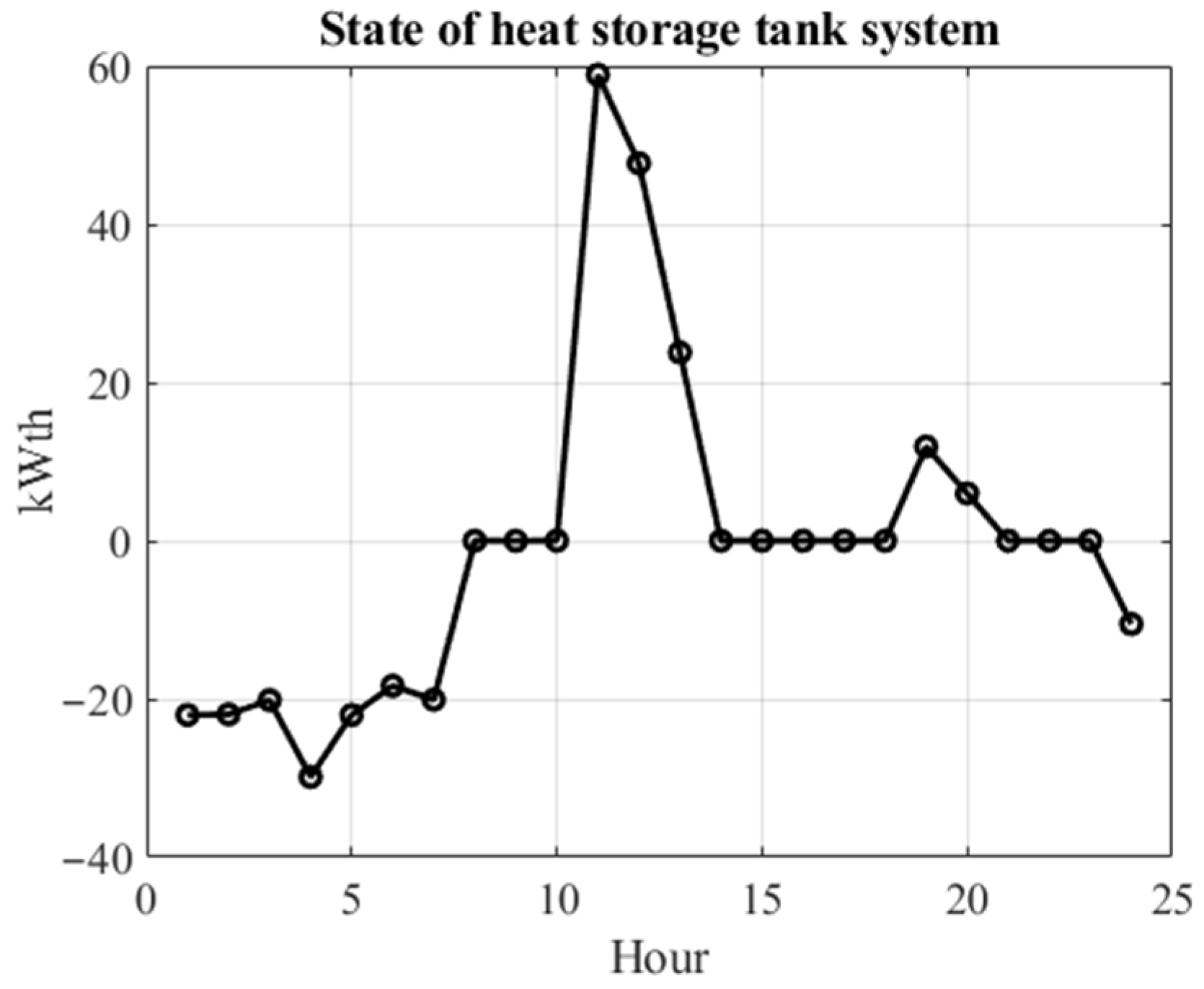
- Battery and Thermal Storage
- (c)
- CHP and P2H Systems
3.1.2. Assumptions of Scenarios
- (a)
- Scenario I: Normal Operating Conditions (No Emergency)
- (b)
- Scenario II: Emergency Load Shedding
- (c)
- Scenario III: Overload Emergency
3.1.3. General Assumptions Across All Scenarios
- (a)
- Fixed System Parameters
- (b)
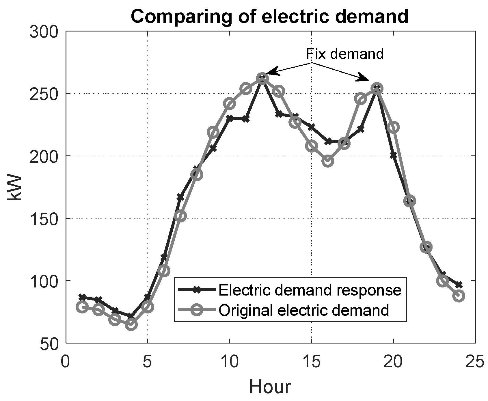
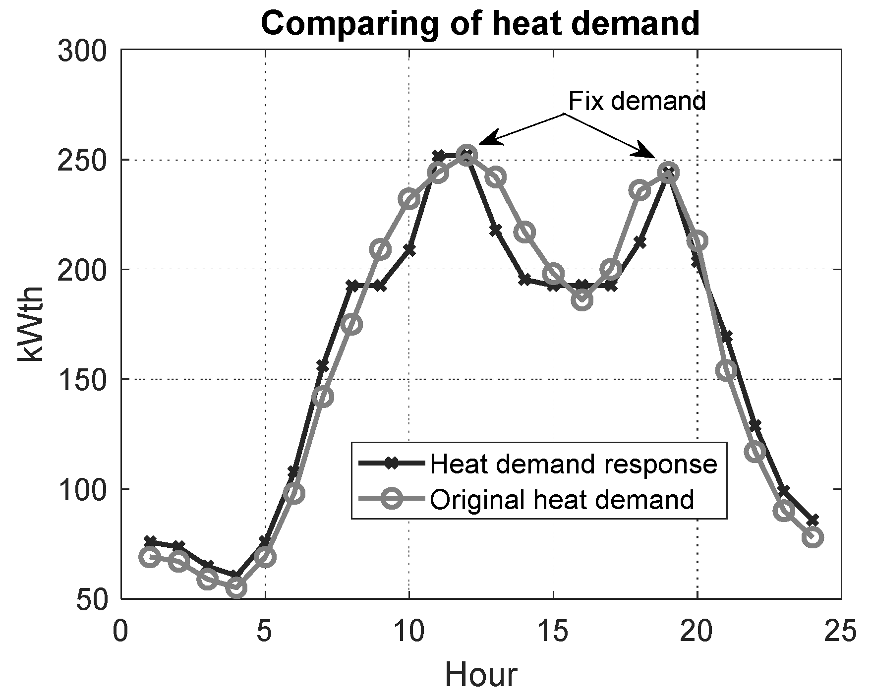
- DRPs
- (c)
- Gurobi Solver
3.2. Scenario I
3.3. Scenario II
3.4. Scenario III
3.5. Comparison and Verification of Results
- Equation (5) is defined as greater or equal in similar articles that have modeled both electrical and thermal energy. In this paper, it was shown that by modeling the DRP and the heat tank, this relationship can be equalized and the heat balance losses between load and production can be reduced to zero;
- Another advantage of the electrical and thermal DRP is that a larger PV can be introduced into the grid to meet the thermal constraint;
- The achievable area of the problem increases with the DRP due to the increase in thermal load and the constraint of equality.
- Lower costs and environmental impact in both normal and emergency conditions.
- Superior emergency handling, particularly in load shedding and overload situations.
- Comprehensive integration of diverse energy sources, including renewables, batteries, and P2H systems, providing flexibility and scalability in real-world applications.
3.6. Sensitivity Analysis
- Base Case (100% of forecasted renewable output),
- Low Renewable Output (80% of forecasted output),
- High Renewable Output (120% of forecasted output).
3.7. Discussion
3.8. Limitations
3.9. Future Research
4. Conclusions
Author Contributions
Funding
Informed Consent Statement
Data Availability Statement
Conflicts of Interest
Abbreviations and Nomenclature
| Nomenclature | |
| The set of number of units (CHP or PV or battery or heat bank) and the time period studied | |
| Fixed coefficient of CHP fuel cost | |
| Fixed coefficient of CHP emission cost | |
| Hourly electrical load of the grid | |
| Hourly heat load of the grid | |
| The hourly electric power of the PV | |
| The percentage amount of flexible thermal and electrical load | |
| Hourly flexible thermal and electrical load amount | |
| The proportionality constant of the CHP in hour | |
| Thermal efficiency and heat exchanger efficiency of the CHP | |
| Thermal rate of the CHP | |
| The maximum power of the CHP unit | |
| The minimum power of the CHP unit | |
| Total efficiency of the battery (battery losses + discharge = charge), depending on the quality of the battery | |
| The total efficiency of the heat bank (heat loss + heat discharge = charge), depends on the heat bank system and the length of the heat transfer pipe | |
| The maximum permissible discharge power of the battery in hour | |
| The maximum permissible charge power of the battery in hour | |
| Maximum permissible discharge of thermal bank in hour | |
| Maximum permissible charge of thermal bank in hour | |
| The cost of starting and shutting down of the CHP units | |
| Total electrical and thermal load shedding capacity | |
| The coefficient of conversion of electrical to heat energy | |
| The maximum electrical power that can be used in the P2H system | |
| Maximum heat capacity of P2H | |
| Thermal efficiency of P2H | |
| The power of the CHP unit at time | |
| Cost and emissions of the CHP at time | |
| The electric load obtained from the DRP | |
| The heat load obtained from the DRP | |
| The heat produced by the CHP unit at time | |
| Discharge and charge of battery at time | |
| Discharge and charge of thermal tank at time | |
| The new power value of PV at time (this means the remaining power from PV after charging the battery) | |
| The wind power per hour | |
| Electrical load shedding and overload at time | |
| Thermal load shedding and overload at time | |
| Electric and thermal energy stored in battery and thermal tank at time | |
| , | The maximum time for unit to be turned on or off consecutively |
| Binary variable of turning on and off the CHP at the time | |
| Binary variable of charging and discharging the battery at the time | |
| Binary variable of charging and discharging the thermal tank at the time | |
| Binary variable of electrical emergency load shedding and overload at the time | |
| Binary variable of thermal emergency load shedding and overload at the time | |
| Binary variable of electrical and thermal DRP (in order to control the time of constant and unchanging loads) | |
| The thermal power injected by the P2H system into the thermal grid | |
| Electric power consumed in the power grid to produce heat in P2H | |
| Heat capacity of P2H system | |
| The final heat power charged in the P2H system | |
| Abbreviation | |
| MILP | Mixed-Integer Linear Programming |
| CHP | Combined heat and power |
| PSO | Particle swarm optimization |
| RER | Renewable energy resource |
| DRP | Demand response program |
| ESS | Energy storage system |
| EV | Electric vehicle |
| PV | Photovoltaic |
| P2H | Power to hydrogen |
| SG | Smart Grid |
| SH | Smart Home |
| BBO | Biogeography-Based Optimization |
| MAE | Mean absolute error |
| NSGA-III | Non-dominated sorting genetic algorithm-III |
| CCG | Column-and-constraint generation |
| TLBO | Teaching–learning-based optimization |
| MBO | Monarch Butterfly Optimization |
| DS | Dynamic simulation |
| GWO | Grey wolf optimization |
References
- Shojaeiyan, S.; Dehghani, M.; Siano, P. Microgrids resiliency enhancement against natural catastrophes based multiple cooperation of water and energy hubs. Smart Cities 2023, 6, 1765–1785. [Google Scholar] [CrossRef]
- Li, D.; Guo, S.; He, W.; King, M.; Wang, J. Combined capacity and operation optimisation of lithium-ion battery energy storage working with a combined heat and power system. Renew. Sustain. Energy Rev. 2021, 140, 110731. [Google Scholar] [CrossRef]
- Zhao, X.; Bai, M.; Yang, X.; Liu, J.; Yu, D.; Chang, J. Short-term probabilistic predictions of wind multi-parameter based on one-dimensional convolutional neural network with attention mechanism and multivariate copula distribution estimation. Energy 2021, 234, 121306. [Google Scholar] [CrossRef]
- Zhou, K.; Fei, Z.; Hu, R. Hybrid robust decentralized optimization of emission-aware multi-energy microgrids considering multiple uncertainties. Energy 2023, 265, 126405. [Google Scholar] [CrossRef]
- Amorim, E.A.; Rocha, C. Optimization of wind-thermal economic-emission dispatch problem using NSGA-III. IEEE Lat. Am. Trans. 2020, 18, 1555–1562. [Google Scholar] [CrossRef]
- Yang, D.; Xu, Y.; Liu, X.; Jiang, C.; Nie, F.; Ran, Z. Economic-emission dispatch problem in integrated electricity and heat system con-sidering multi-energy demand response and carbon capture Technologies. Energy 2022, 253, 124153. [Google Scholar] [CrossRef]
- Ellahi, M.; Abbas, G.; Satrya, G.B.; Usman, M.R.; Gu, J. A Modified hybrid particle swarm optimization with bat algorithm parameter inspired acceleration coefficients for solving eco-friendly and economic dispatch problems. IEEE Access 2021, 9, 82169–82187. [Google Scholar] [CrossRef]
- Ellahi, M.; Abbas, G. A hybrid metaheuristic approach for the solution of renewables-incorporated economic dispatch problems. IEEE Access 2020, 8, 127608–127621. [Google Scholar] [CrossRef]
- Lu, S.; Gu, W.; Meng, K.; Dong, Z.Y. Economic dispatch of integrated energy systems with robust thermal comfort management. IEEE Trans. Sustain. Energy 2020, 12, 222–233. [Google Scholar] [CrossRef]
- Zhu, Z.; Wang, M.; Xing, Z.; Liu, Y.; Chen, S. Optimal configuration of power/thermal energy storage for a park-integrated energy system considering flexible load. Energies 2023, 16, 6424. [Google Scholar] [CrossRef]
- Khobaragade, T.; Chaturvedi, K.T. Enhanced Economic Load Dispatch by Teaching–Learning-Based Optimization (TLBO) on Thermal Units: A Comparative Study with Different Plug-in Electric Vehicle (PEV) Charging Strategies. Energies 2023, 16, 6933. [Google Scholar] [CrossRef]
- Huang, Q.; Han, S.; Rong, N.; Luo, J.; Hu, X. Stochastic economic dispatch of hydro-thermal-wind-photovoltaic power system con-sidering mixed coal-blending combustion. IEEE Access 2020, 8, 218542–218553. [Google Scholar] [CrossRef]
- Wang, Y.; Jin, J.; Liu, H.; Zhang, Z.; Liu, S.; Ma, J.; Gong, C.; Zheng, Y.; Lin, Z.; Yang, L. The optimal emergency demand response (EDR) mechanism for rural power grid considering consumers’ satisfaction. Energy Rep. 2021, 7, 118–125. [Google Scholar] [CrossRef]
- Han, J.; Yan, L.; Li, Z.; Zhang, L.; Paaso, A.; Bahramirad, S. A Multi-timescale two-stage robust grid-friendly dispatch model for microgrid operation. IEEE Access 2020, 8, 74267–74279. [Google Scholar] [CrossRef]
- Siqin, Z.; Niu, D.; Wang, X.; Zhen, H.; Li, M.; Wang, J. A two-stage distributionally robust optimization model for P2G-CCHP microgrid considering uncertainty and carbon emission. Energy 2022, 260, 124796. [Google Scholar] [CrossRef]
- Valipour, E.; Nourollahi, R.; Taghizad-Tavana, K.; Nojavan, S.; Alizadeh, A. Risk assessment of industrial energy hubs and peer-to-peer heat and power transaction in the presence of electric vehicles. Energies 2022, 15, 8920. [Google Scholar] [CrossRef]
- Li, Z.; Wu, L.; Xu, Y.; Zheng, X. Stochastic-weighted robust optimization based bilayer operation of a multi-energy building microgrid considering practical thermal loads and battery degradation. IEEE Trans. Sustain. Energy 2021, 13, 668–682. [Google Scholar] [CrossRef]
- Akhlaghi, M.; Moravej, Z.; Bagheri, A. Maximizing wind energy utilization in smart power systems using a flexible net-work-constrained unit commitment through dynamic lines and transformers rating. Energy 2022, 261, 124918. [Google Scholar] [CrossRef]
- Ahmadi, E.; Noorollahi, Y.; Mohammadi-Ivatloo, B.; Anvari-Moghaddam, A. Stochastic operation of a solar-powered smart home: Capturing thermal load uncertainties. Sustainability 2020, 12, 5089. [Google Scholar] [CrossRef]
- Askari, M.; Dehghani, M.; Razmjoui, P.; GhasemiGarpachi, M.; Tahmasebi, D.; Ghasemi, S. A novel stochastic thermo-solar model for water demand supply using point estimate method. IET Renew. Power Gener. 2022, 16, 3559–3572. [Google Scholar] [CrossRef]
- Hussain, A.; Bui, V.-H.; Kim, H.-M.; Im, Y.-H.; Lee, J.-Y. Optimal energy management of combined cooling, heat and power in different demand type buildings considering seasonal demand variations. Energies 2017, 10, 789. [Google Scholar] [CrossRef]
- Haghighat, H.; Karimianfard, H.; Zeng, B. Integrating energy management of autonomous smart grids in electricity market operation. IEEE Trans. Smart Grid 2020, 11, 4044–4055. [Google Scholar] [CrossRef]
- Kumar, S.; Krishnasamy, V.; Kaur, R.; Kandasamy, N.K. Virtual energy storage-based energy management algorithm for optimally sized DC nanogrid. IEEE Syst. J. 2021, 16, 231–239. [Google Scholar] [CrossRef]
- Zhao, W.; Diao, H.; Li, P.; Lv, X.; Lei, E.; Mao, Z.; Xue, W. Transactive energy-based joint optimization of energy and flexible reserve for integrated electric-heat systems. IEEE Access 2021, 9, 14491–14503. [Google Scholar] [CrossRef]
- Maghanki, M.M.; Ghobadian, B.; Najafi, G.; Galogah, R.J. Micro combined heat and power (MCHP) technologies and applications. Renew. Sustain. Energy Rev. 2013, 28, 510–524. [Google Scholar] [CrossRef]
- Daramola, A.S.; Ahmadi, S.E.; Marzband, M.; Ikpehai, A. A cost-effective and ecological stochastic optimization for integration of distributed energy resources in energy networks considering vehicle-to-grid and combined heat and power technologies. J. Energy Storage 2022, 57, 106203. [Google Scholar] [CrossRef]
- Zhang, G.; Ge, Y.; Ye, Z.; Al-Bahrani, M. Multi-objective planning of energy hub on economic aspects and resources with heat and power sources, energizable, electric vehicle and hydrogen storage system due to uncertainties and demand response. J. Energy Storage 2022, 57, 106160. [Google Scholar] [CrossRef]
- Karimianfard, H.; Haghighat, H.; Zeng, B. Co-optimization of battery storage investment and grid expansion in integrated energy systems. IEEE Syst. J. 2021, 16, 5928–5938. [Google Scholar] [CrossRef]
- Battula, A.R.; Vuddanti, S.; Salkuti, S.R. A day ahead demand schedule strategy for optimal operation of microgrid with uncertainty. Smart Cities 2023, 6, 491–509. [Google Scholar] [CrossRef]
- Ntafalias, A.; Tsakanikas, S.; Skarvelis-Kazakos, S.; Papadopoulos, P.; Skarmeta-Gómez, A.F.; González-Vidal, A.; Tomat, V.; Ramallo-González, A.P.; Marin-Perez, R.; Vlachou, M.C. Design and Implementation of an Interoperable Architecture for Integrating Building Legacy Systems into Scalable Energy Management Systems. Smart Cities 2022, 5, 1421–1440. [Google Scholar] [CrossRef]
- Razghandi, M.; Zhou, H.; Erol-Kantarci, M.; Turgut, D. Smart Home Energy Management: VAE-GAN Synthetic Dataset Generator and Q-Learning. IEEE Trans. Smart Grid 2023, 15, 1562–1573. [Google Scholar] [CrossRef]
- Wang, Y.; Chen, C.F.; Kong, P.Y.; Li, H.; Wen, Q. A cyber–physical–social perspective on future smart distribution systems. Proc. IEEE 2022, 111, 694–724. [Google Scholar] [CrossRef]
- Shokri, M.; Niknam, T.; Mohammadi, M.; Dehghani, M.; Siano, P.; Ouahada, K.; Sarvarizade-Kouhpaye, M. A novel stochastic framework for optimal scheduling of smart cities as an energy hub. IET Gener. Transm. Distrib. 2024, 18, 2421–2434. [Google Scholar] [CrossRef]
- Eltamaly, A.M. Optimal Dispatch Strategy for Electric Vehicles in V2G Applications. Smart Cities 2023, 6, 3161–3191. [Google Scholar] [CrossRef]
- Shibu, N.S.; Devidas, A.R.; Balamurugan, S.; Ponnekanti, S.; Ramesh, M.V. Optimising Microgrid Resilience: Integrating IoT, Blockchain, and Smart Contracts for Power Outage Management. IEEE Access 2024, 12, 18782–18803. [Google Scholar] [CrossRef]
- Pati, U.; Mistry, K.D. Cyber-Resilient Trading for Sustainable Energy Management: A Three-Phase Demand-Side Management Solution with Integrated Deep Learning-Based Renewable Energy Forecasting. IEEE Trans. Ind. Appl. 2023, 60, 2532–2541. [Google Scholar] [CrossRef]
- Azarinfar, H.; Khosravi, M.; Sabzevari, K.; Dzikuć, M. Stochastic Economic–Resilience Management of Combined Cooling, Heat, and Power-Based Microgrids in a Multi-Objective Approach. Sustainability 2024, 16, 1212. [Google Scholar] [CrossRef]
- Nasab, M.A.; Zand, M.; Eskandari, M.; Sanjeevikumar, P.; Siano, P. Optimal planning of electrical appliance of residential units in a smart home network using cloud services. Smart Cities 2021, 4, 1173–1195. [Google Scholar] [CrossRef]
- Jokar, H.; Niknam, T.; Dehghani, M.; Sheybani, E.; Pourbehzadi, M.; Javidi, G. Efficient Microgrid Management with Meerkat Opti-mization for Energy Storage, Renewables, Hydrogen Storage, Demand Response, and EV Charging. Energies 2023, 17, 25. [Google Scholar] [CrossRef]
- Fan, Z.; Cao, J.; Jamal, T.; Fogwill, C.; Samende, C.; Robinson, Z.; Polack, F.; Ormerod, M.; George, S.; Peacock, A.; et al. The role of ‘living laboratories’ in accelerating the energy system decarbonization. Energy Rep. 2022, 8, 11858–11864. [Google Scholar] [CrossRef]
- Basu, A.K.; Bhattacharya, A.; Chowdhury, S. Planned scheduling for economic power sharing in a CHP-based micro-grid. IEEE Trans. Power Syst. 2011, 27, 30–38. [Google Scholar] [CrossRef]
- Yan, M.; Teng, F.; Gan, W.; Yao, W.; Wen, J. Blockchain for secure decentralized energy management of multi-energy system using state machine replication. Appl. Energy 2023, 337, 120863. [Google Scholar] [CrossRef]
- Gourisetti, S.N.G.; Sebastian-Cardenas, D.J.; Bhattarai, B.; Wang, P.; Widergren, S.; Borkum, M.; Randall, A. Blockchain smart contract reference framework and program logic architecture for transactive energy systems. Appl. Energy 2021, 304, 117860. [Google Scholar] [CrossRef]
- Christidis, K.; Sikeridis, D.; Wang, Y.; Devetsikiotis, M. A framework for designing and evaluating realistic blockchain-based local energy markets. Appl. Energy 2021, 281, 115963. [Google Scholar] [CrossRef]
- Li, Y.; Yang, W.; He, P.; Chen, C.; Wang, X. Design and management of a distributed hybrid energy system through smart contract and blockchain. Appl. Energy 2019, 248, 390–405. [Google Scholar] [CrossRef]
- Khalid, R.; Javaid, N.; Javaid, S.; Imran, M.; Naseer, N. A blockchain-based decentralized energy management in a P2P trading system. In Proceedings of the ICC 2020—2020 IEEE International Conference on Communications (ICC), Dublin, Ireland, 7–11 June 2020; pp. 1–6. [Google Scholar]


| Ref. | Solver | Model | ELM | Emission Reduction | DR | CHP | P2H | Battery Integration | Thermal Storage | Relevance to This Study |
|---|---|---|---|---|---|---|---|---|---|---|
| This Paper | Gurobi | MILP | Yes | Yes | Yes | Yes | Yes | Yes | Yes | Comprehensive multi-source energy management under emergency conditions, focusing on CHP, P2H, and DR. |
| [2] | BBO | NLP | No | Yes | Yes | Yes | No | Yes | No | Limited to emission reduction and DR, lacks emergency load and P2H integration. |
| [3] | MAE | NLP | No | No | No | No | No | No | No | Focused on renewable integration but lacks CHP, DR, and ELM. |
| [4] | Gurobi | MILP | No | No | Yes | Yes | Yes | Yes | Yes | Similar MILP-based model but no focus on emergency conditions, limiting relevance for load emergencies. |
| [5] | NSGA-III | NLP | No | Yes | No | No | No | No | No | Focused on emission reduction, lacks comprehensive energy management, emergency handling, and thermal storage integration. |
| [6] | Gurobi | MILP | No | Yes | Yes | Yes | No | No | Yes | Limited focus on CHP and renewables, lacks P2H and emergency load scenarios. |
| [7] | PSO | NLP | No | Yes | No | No | No | No | No | Economic and environmental optimization but lacks emergency management and thermal integration. |
| [8] | PSO-BAT | NLP | No | Yes | No | No | No | No | No | Hybrid approach to thermal plants, lacks renewable and storage integration. |
| [9] | CCG | MILP | No | Yes | Yes | No | No | Yes | Yes | Economic load distribution amid uncertainties, limited scope on CHP and storage. |
| [10] | - | MILP | No | No | No | No | No | Yes | Yes | Focus on steam extraction for better energy management, lacks comprehensive energy sources. |
| [11] | TLBO | NLP | No | Yes | No | No | No | No | No | Addresses wind power and load uncertainties but lacks comprehensive renewable and DR integration. |
| [12] | MBO | NLP | No | Yes | No | No | No | No | Yes | Stochastic model for heat and hydro-PV, lacks CHP and emergency management. |
| [13] | GA | NLP | Yes | No | Yes | Yes | No | Yes | Yes | Optimizes microgrids with electrical and gas sources, lacks CHP and thermal integration. |
| [14] | Gurobi | MIP | No | No | No | Yes | No | Yes | No | Focuses on renewable and load uncertainties, lacks ELM. |
| [15] | Cplex | MILP | No | Yes | Yes | Yes | Yes | Yes | Yes | Model for heating and cooling optimization, no emphasis on emergencies or renewables. |
| [16] | Cplex | MILP | No | Yes | Yes | Yes | No | Yes | Yes | Considers uncertainties in EV loads, lacks comprehensive thermal integration. |
| [17] | Cplex | MILP | No | Yes | Yes | Yes | Yes | Yes | Yes | Microgrid coordination but no CHP or P2H integration. |
| [18] | Heuristic | MINLP | No | No | Yes | No | No | Yes | No | Focuses on unit participation in energy systems, lacks CHP and DR programs. |
| [19] | Cplex | MILP | No | Yes | Yes | Yes | No | Yes | Yes | Thermal and electrical scheduling, lacks emergency management. |
| [20] | - | NLP | No | No | No | No | No | Yes | No | Stochastic solar thermal model, lacks CHP integration. |
| [21] | DS | NLP | No | Yes | Yes | Yes | No | Yes | Yes | Dynamic simulation of thermal and electrical energy management, lacks emergency handling. |
| [22] | CCG | MICP | No | Yes | Yes | No | No | No | No | Optimal load and energy operation in grids but lacks emergency load scenarios. |
| [23] | GWO | NLP | No | No | No | No | No | No | No | Energy management algorithm for DC nanogrids but lacks CHP or emergency load focus. |
| [24] | CCG | MILP | No | No | Yes | Yes | No | No | No | Energy distribution in thermoelectric systems, lacks comprehensive emergency handling. |
| [25] | - | NLP | No | No | No | Yes | No | No | Yes | Explores feasibility of CHP systems, lacks P2H integration. |
| [26] | - | MILP | No | Yes | Yes | No | No | Yes | Yes | Optimizes distributed energy but lacks emergency load handling. |
| [27] | Heuristic | NLP | No | Yes | Yes | Yes | No | Yes | Yes | Multi-objective planning for energy hubs, lacks emergency focus. |
| [28] | CCG | MILP | No | No | Yes | No | No | Yes | Yes | Focuses on electricity and gas transmission grids, lacks emergency management. |
| CHP1 | CHP2 | CHP3 | CHP4 | |
|---|---|---|---|---|
| 2.035 | 0.5768 | 1.1825 | 0.338 | |
| 60.28 | 57.783 | 65.34 | 89.1476 | |
| 44 | 133.0915 | 44 | 547.619 | |
| 14.4296 | 3.0358 | 19.38 | 1.0346 | |
| 64.1535 | 57.3403 | 176.6946 | 60.384 | |
| 130.4094 | 311.5728 | 821.6573 | 943.1898 | |
| 400 | 200 | 300 | 100 | |
| 300 | 100 | 200 | 50 | |
| 11041 | 11373 | 10581 | 12186 | |
| 0.3 | 0.5 | 0.3 | 0.5 | |
| 0.9 | 0.9 | 0.9 | 0.9 | |
| ESS | ||||
| 56 | 70 | 250 | 0.9 | |
| Heat storage tank | ||||
| 160 | 200 | 400 | 0.9 | |
| Electric and thermal DR | ||||
| 0.1 | 0.1 | |||
| CHP1 | CHP2 | CHP3 | CHP4 | |
|---|---|---|---|---|
| Min up time | 1 | 1 | 1 | 1 |
| Min down time | 1 | 0 | 1 | 0 |
| Ramp up rate | 45 | 20 | 40 | 10 |
| Ramp down rate | 45 | 20 | 40 | 10 |
| Heat Storage Tank | Battery | ||
|---|---|---|---|
| 10 | 13 | ||
| 5 | 6 | ||
| 400 kWhth | 250 kWh | ||
| h | (kWh) | (kWhth) | (kWh) | (kWh) | h | (kWh) | (kWhth) | (kWh) | (kWh) |
|---|---|---|---|---|---|---|---|---|---|
| 1 | 79 | 69 | 0 | 1.8 | 13 | 252 | 242 | 52 | 17.0 |
| 2 | 77 | 67 | 0 | 1.5 | 14 | 227 | 217 | 50 | 18.0 |
| 3 | 69 | 59 | 0 | 1.2 | 15 | 208 | 198 | 48 | 19.0 |
| 4 | 65 | 55 | 0 | 1.0 | 16 | 196 | 186 | 46 | 20.0 |
| 5 | 79 | 69 | 0 | 1.0 | 17 | 210 | 200 | 32 | 20.0 |
| 6 | 108 | 98 | 0 | 2.5 | 18 | 246 | 236 | 16 | 18.0 |
| 7 | 152 | 142 | 8 | 4.0 | 19 | 254 | 244 | 8 | 16.0 |
| 8 | 185 | 175 | 16 | 6.0 | 20 | 223 | 213 | 0 | 14.0 |
| 9 | 219 | 209 | 32 | 8.0 | 21 | 164 | 154 | 0 | 12.0 |
| 10 | 242 | 232 | 46 | 10.0 | 22 | 127 | 117 | 0 | 8.0 |
| 11 | 254 | 244 | 48 | 12.0 | 23 | 100 | 90 | 0 | 5.0 |
| 12 | 262 | 252 | 50 | 15.0 | 24 | 88 | 78 | 0 | 2.0 |
| Hour | (kWh) | (kWh) | (kWh) | (kWh) | (kWh) | (kWh) | (kWh) | (kWh) | (kWh) | (kWh) |
|---|---|---|---|---|---|---|---|---|---|---|
| 1 | 44.14 | 30.47 | 0 | 10.20 | 86.9 | 79 | 0 | 2.0 | 0 | 0 |
| 2 | 42.8 | 30 | 0 | 10.03 | 84.7 | 77 | 0 | 1.8 | 0 | 0 |
| 3 | 39.5 | 26.1 | 0 | 8.79 | 75.9 | 69 | 0 | 1.5 | 0 | 0 |
| 4 | 0.0 | 38.3 | 20 | 12.38 | 71.5 | 65 | 0 | 1.2 | 0 | 0 |
| 5 | 44.47 | 31.13 | 0 | 10.20 | 86.9 | 79 | 0 | 1.0 | 0 | 0 |
| 6 | 52.37 | 34.23 | 20 | 11.12 | 118.8 | 108 | 0 | 1.0 | 0 | 0 |
| 7 | 83.97 | 45.73 | 20 | 14.8 | 167.2 | 152 | 0 | 2.5 | 8 | 0 |
| 8 | 93.57 | 48.9 | 20 | 16.1 | 189.6 | 185 | 6.85 | 4.0 | 9.14 | 0 |
| 9 | 93.0 | 47.6 | 20 | 16.1 | 206 | 219 | 23.3 | 6.0 | 8.66 | 0 |
| 10 | 100.34 | 51.37 | 20.1 | 17.7 | 230 | 242 | 32.6 | 8.0 | 13.3 | 0 |
| 11 | 91.67 | 44.9 | 20 | 16.1 | 229 | 254 | 46.87 | 10.0 | 1.13 | 0 |
| 12 | 98.0 | 46.9 | 20 | 17.13 | 262 | 262 | 50 | 12.0 | 0 | 18.27 |
| 13 | 90.6 | 42 | 20 | 16.2 | 233 | 252 | 49.48 | 15.0 | 2.51 | 0 |
| 14 | 90.33 | 41.2 | 20 | 16.4 | 231 | 227 | 46.1 | 17.0 | 3.88 | 0 |
| 15 | 89.0 | 39.7 | 20 | 16.1 | 223. | 208 | 40.2 | 18.0 | 7.765 | 0 |
| 16 | 88.67 | 38.9 | 20 | 16.1 | 211 | 196 | 28.88 | 19.0 | 17.12 | 0 |
| 17 | 88.33 | 38.27 | 20 | 16.1 | 211.2 | 210 | 28.3 | 20.0 | 3.60 | 0 |
| 18 | 98.33 | 43.97 | 20.6 | 17.9 | 221.4 | 246 | 16 | 20.0 | 0 | 4.17 |
| 19 | 109.0 | 50.8 | 22.5 | 19.6 | 254 | 254 | 8 | 18.0 | 0 | 26.3 |
| 20 | 92.77 | 42.13 | 20 | 16.4 | 200.7 | 223 | 0 | 16.0 | 0 | 13.1 |
| 21 | 79.33 | 35.37 | 20 | 13.7 | 162 | 164 | 0 | 14.0 | 0 | 0 |
| 22 | 60.8 | 23.3 | 20 | 9.62 | 125 | 127 | 0 | 12.0 | 0 | 0 |
| 23 | 48.0 | 16.47 | 20 | 6.601 | 104.8 | 100 | 0 | 8.0 | 0 | 5.65 |
| 24 | 47.73 | 17.67 | 20 | 6.332 | 96.7 | 88 | 0 | 5.0 | 0 | 0.005 |
| Total | 1766.7 | 905.5 | 403.3 | 332.3 | 4086 | 4086 | 376.8 | 233 | 75.1 | 67.629 |
| Hour | (kWhth) | (kWhth) | (kWhth) | (kWhth) | (kWhth) | |||||
| 1 | 97.9 | 22.03 | 0 | 75.9 | 69 | 287 | 68 | 355 | ||
| 2 | 95.6 | 21.95 | 0 | 73.7 | 67 | 274 | 65 | 339 | ||
| 3 | 85.0 | 20.15 | 0 | 64.9 | 59 | 216 | 52 | 268 | ||
| 4 | 90.3 | 29.84 | 0 | 60.5 | 55 | 311 | 96 | 407 | ||
| 5 | 97.9 | 22.03 | 0 | 75.9 | 69 | 287 | 68 | 355 | ||
| 6 | 126.1 | 18.34 | 0 | 107.8 | 98 | 379 | 120 | 499 | ||
| 7 | 176.2 | 20.09 | 0 | 156.2 | 142 | 767 | 219 | 986 | ||
| 8 | 192.5 | 0 | 0 | 192.5 | 175 | 924 | 259 | 1183 | ||
| 9 | 192.6 | 0.01 | 0 | 192.6 | 209 | 925 | 260 | 1185 | ||
| 10 | 208.8 | 0 | 0 | 208.8 | 232 | 1097 | 302 | 1399 | ||
| 11 | 192.6 | 0 | 58.9 | 251.5 | 244 | 925 | 260 | 1185 | ||
| 12 | 204.2 | 0 | 47.7 | 252 | 252 | 1048 | 291 | 1339 | ||
| 13 | 193.9 | 0 | 23.8 | 217.8 | 242 | 939 | 263 | 1202 | ||
| 14 | 195.3 | 0 | 0 | 195.3 | 217 | 953 | 267 | 1220 | ||
| 15 | 192.6 | 0 | 0 | 192.6 | 198 | 925 | 260 | 1185 | ||
| 16 | 192.6 | 0 | 0 | 192.6 | 186 | 925 | 260 | 1185 | ||
| 17 | 192.6 | 0 | 0 | 192.6 | 200 | 925 | 260 | 1185 | ||
| 18 | 212.4 | 0 | 0 | 212.4 | 236 | 1133 | 314 | 1447 | ||
| 19 | 232 | 0 | 11.9 | 244 | 244 | 1352 | 374 | 1726 | ||
| 20 | 197.4 | 0 | 5.97 | 203.4 | 213 | 975 | 273 | 1248 | ||
| 21 | 169.4 | 0 | 0 | 169.4 | 154 | 704 | 205 | 909 | ||
| 22 | 128.7 | 0 | 0 | 128.7 | 117 | 392 | 128 | 520 | ||
| 23 | 99 | 0 | 0 | 99 | 90 | 225 | 86 | 311 | ||
| 24 | 96.32 | 10.52 | 0 | 85.8 | 78 | 213 | 83 | 296 | ||
| Total | 3863 | 164.9 | 148.4 | 3846 | 3846 | 17,101 | 4833 | 21,934 | ||
| Hour | (kWh) | (kWh) | (kWh) | (kWh) | (kWh) | (kWh) | (kWh) | (kWh) |
|---|---|---|---|---|---|---|---|---|
| 1 | 46.996 | 30.279 | 0 | 9.6243 | 86.9 | 0 | 0 | 0 |
| 2 | 45.539 | 29.708 | 0 | 9.4538 | 84.7 | 0 | 0 | 0 |
| 3 | 40 | 27.195 | 0 | 8.7044 | 75.9 | 0 | 0 | 0 |
| 4 | 0 | 38.441 | 20 | 12.058 | 70.499 | 0 | 0 | 0 |
| 5 | 45 | 31.817 | 0 | 10.083 | 86.9 | 0 | 0 | 0 |
| 6 | 54.881 | 33.372 | 20 | 10.547 | 118.8 | 0 | 0 | 0 |
| 7 | 67.803 | 38.44 | 20 | 12.059 | 138.3 | 0 | 8 | 0 |
| 8 | 84.302 | 44.911 | 20 | 13.989 | 166.5 | 3.2985 | 12.702 | 0 |
| 9 | 92.472 | 50.413 | 20 | 15.747 | 197.1 | 18.468 | 13.532 | 0 |
| 10 | 102.26 | 57.001 | 20.034 | 17.852 | 217.8 | 20.658 | 25.342 | 0 |
| 11 | 95.279 | 49.833 | 20 | 15.488 | 228.6 | 48 | 0 | 0 |
| 12 | 96.347 | 50.252 | 20 | 15.613 | 262 | 50 | 0 | 29.788 |
| 13 | 82.734 | 44.913 | 20 | 14.02 | 226.8 | 52 | 0 | 13.132 |
| 14 | 94.11 | 53.429 | 20 | 16.768 | 204.3 | 19.993 | 30.007 | 0 |
| 15 | 86.018 | 47.981 | 20 | 15.026 | 187.2 | 18.175 | 29.825 | 0 |
| 16 | 80.907 | 44.539 | 20 | 13.927 | 176.4 | 17.027 | 28.973 | 0 |
| 17 | 86.87 | 48.554 | 20 | 15.21 | 189 | 18.367 | 13.633 | 0 |
| 18 | 82.734 | 44.913 | 20 | 14.02 | 221.4 | 16 | 0 | 43.732 |
| 19 | 107.36 | 60.863 | 21.002 | 19.099 | 254 | 8 | 0 | 37.68 |
| 20 | 94.2 | 51.55 | 20 | 16.11 | 200.7 | 0 | 0 | 18.84 |
| 21 | 72.216 | 40.171 | 20 | 12.575 | 147.6 | 0 | 0 | 2.639 |
| 22 | 60.074 | 33.236 | 20 | 10.395 | 123.7 | 0 | 0 | 0 |
| 23 | 53.53 | 28.829 | 0 | 8.9868 | 91.346 | 0 | 0 | 0 |
| 24 | 47.283 | 24.623 | 0 | 7.6425 | 79.549 | 0 | 0 | 0 |
| Total | 1718.9 | 1005.3 | 361.04 | 315 | 3836 | 289.99 | 162.01 | 145.81 |
| Hour | (kWhth) | (kWhth) | (kWhth) | (kWhth) | (kWhth) | (kWhth) | ||
| 1 | 96.623 | 34.333 | 0 | 62.29 | 0 | 0 | 236 | |
| 2 | 94.343 | 33.853 | 0 | 60.49 | 0 | 0 | 225 | |
| 3 | 85.044 | 31.754 | 0 | 53.29 | 0 | 0 | 183 | |
| 4 | 88.887 | 39.198 | 0 | 49.69 | 0 | 0 | 308 | |
| 5 | 97.854 | 35.565 | 0 | 62.289 | 0 | 0 | 242 | |
| 6 | 124.83 | 36.435 | 0 | 88.39 | 0 | 0 | 388 | |
| 7 | 145.03 | 17.041 | 0 | 127.99 | 0 | 0 | 511 | |
| 8 | 170.84 | 0 | 0 | 170.83 | 0 | 0 | 700 | |
| 9 | 188.1 | 0 | 0 | 188.1 | 0 | 0 | 841 | |
| 10 | 208.8 | 0 | 0 | 208.8 | 0 | 0 | 1030 | |
| 11 | 189.21 | 0 | 30.394 | 219.6 | 0 | 0 | 854 | |
| 12 | 190.88 | 0 | 61.124 | 252 | 0 | 0 | 869 | |
| 13 | 169.59 | 0 | 48.213 | 217.8 | 0 | 0 | 688 | |
| 14 | 195.3 | 0 | 0 | 195.3 | 0 | 0 | 901 | |
| 15 | 178.2 | 0 | 0 | 178.2 | 0 | 0 | 755 | |
| 16 | 167.4 | 0 | 0 | 167.4 | 0 | 0 | 671 | |
| 17 | 180 | 0 | 0 | 180 | 0 | 0 | 770 | |
| 18 | 169.59 | 0 | 42.813 | 212.4 | 10 | 10 | 688 | |
| 19 | 221.18 | 0 | 22.818 | 244 | 0 | 0 | 1153 | |
| 20 | 191.7 | 0 | 0 | 191.7 | 60 | 60 | 872 | |
| 21 | 151.93 | 0 | 0 | 151.93 | 60 | 60 | 558 | |
| 22 | 128.7 | 0 | 0 | 128.7 | 60 | 60 | 412 | |
| 23 | 99 | 0 | 0 | 99 | 60 | 60 | 251 | |
| 24 | 85.8 | 0 | 0 | 85.8 | 0 | 0 | 189 | |
| Total | 3618.8 | 228.18 | 205.36 | 3596 | 250 | 250 | 14,295 | |
| Hour | (kWh) | (kWh) | (kWh) | (kWh) | (kWh) | (kWh) | (kWh) | (kWh) |
|---|---|---|---|---|---|---|---|---|
| 1 | 51.821 | 26.776 | 0 | 8.3035 | 86.9 | 0 | 0 | 0 |
| 2 | 50.363 | 26.204 | 0 | 8.133 | 84.7 | 0 | 0 | 0 |
| 3 | 44.532 | 23.917 | 0 | 7.4509 | 75.9 | 0 | 0 | 0 |
| 4 | 0 | 39.424 | 20 | 12.076 | 71.5 | 0 | 0 | 0 |
| 5 | 45 | 32.029 | 0 | 9.8707 | 86.9 | 0 | 0 | 0 |
| 6 | 59.706 | 29.868 | 20 | 9.226 | 118.8 | 0 | 0 | 0 |
| 7 | 91.775 | 42.447 | 20 | 12.978 | 167.2 | 0 | 8 | 0 |
| 8 | 108.99 | 49.197 | 21.698 | 14.991 | 203.5 | 8.6277 | 7.3723 | 0 |
| 9 | 116.82 | 52.746 | 23.261 | 16.074 | 240.9 | 32 | 0 | 0 |
| 10 | 120.29 | 54.108 | 23.961 | 16.48 | 260.84 | 46 | 0 | 0 |
| 11 | 115.11 | 50.621 | 22.961 | 15.366 | 252.06 | 48 | 0 | 0 |
| 12 | 115.92 | 51.166 | 23.117 | 15.54 | 262 | 50 | 0 | 6.2553 |
| 13 | 120.29 | 54.108 | 23.961 | 16.48 | 269.27 | 52 | 0 | 2.436 |
| 14 | 111.44 | 50.637 | 22.178 | 15.445 | 249.7 | 50 | 0 | 0 |
| 15 | 110.68 | 50.341 | 22.026 | 15.357 | 228.8 | 30.392 | 17.608 | 0 |
| 16 | 110.68 | 50.34 | 22.026 | 15.357 | 215.6 | 17.195 | 28.805 | 0 |
| 17 | 111.03 | 50.477 | 22.096 | 15.397 | 231 | 31.999 | 0 | 0 |
| 18 | 120.29 | 54.108 | 23.961 | 16.48 | 230.84 | 16 | 0 | 0 |
| 19 | 126.04 | 57.982 | 25.072 | 17.719 | 254 | 8 | 0 | 19.186 |
| 20 | 120.29 | 54.107 | 23.961 | 16.48 | 229.64 | 0 | 0 | 14.8 |
| 21 | 97.524 | 38.779 | 20 | 11.581 | 176.04 | 0 | 0 | 8.1577 |
| 22 | 78.264 | 25.81 | 20 | 7.4366 | 136.28 | 0 | 0 | 4.7733 |
| 23 | 64.373 | 16.456 | 20 | 6 | 106.83 | 0 | 0 | 0 |
| 24 | 54.8 | 16 | 20 | 6 | 96.8 | 0 | 0 | 0 |
| Total | 2146 | 997.65 | 440.28 | 306.23 | 4336 | 390.2170 | 61.787 | 55.608 |
| Hour | (kWhth) | (kWhth) | (kWhth) | (kWhth) | (kWhth) | (kWhth) | ||
| 1 | 93.625 | 17.725 | 0 | 75.9 | 0 | 0 | 301 | |
| 2 | 91.345 | 17.645 | 0 | 73.7 | 0 | 0 | 286 | |
| 3 | 82.226 | 17.326 | 0 | 64.9 | 0 | 20 | 231 | |
| 4 | 90.312 | 29.813 | 0 | 60.5 | 0 | 20 | 422 | |
| 5 | 97.833 | 21.933 | 0 | 75.9 | 20 | 20 | 322 | |
| 6 | 121.83 | 14.027 | 0 | 107.8 | 20 | 20 | 503 | |
| 7 | 171.98 | 15.78 | 0 | 156.2 | 20 | 20 | 964 | |
| 8 | 200.24 | 7.7412 | 0 | 192.5 | 20 | 0 | 1306 | |
| 9 | 214.66 | 0 | 0 | 214.66 | 20 | 10 | 1500 | |
| 10 | 220.65 | 0 | 0 | 220.65 | 20 | 20 | 1586 | |
| 11 | 208.91 | 0 | 59.488 | 268.4 | 0 | 20 | 1429 | |
| 12 | 210.75 | 0 | 41.251 | 252 | 0 | 0 | 1453 | |
| 13 | 220.65 | 0 | 20.626 | 241.27 | 0 | 0 | 1586 | |
| 14 | 205.39 | 0 | 0 | 205.39 | 0 | 0 | 1372 | |
| 15 | 204.09 | 0 | 0 | 204.09 | 0 | 0 | 1354 | |
| 16 | 204.09 | 0 | 0 | 204.09 | 10 | 0 | 1354 | |
| 17 | 204.69 | 0 | 0 | 204.69 | 20 | 0 | 1362 | |
| 18 | 220.65 | 0 | 0 | 220.65 | 20 | 0 | 1586 | |
| 19 | 233.69 | 0 | 10.313 | 244 | 0 | 0 | 1770 | |
| 20 | 220.65 | 0 | 5.1564 | 225.8 | 20 | 0 | 1586 | |
| 21 | 169.4 | 0 | 0 | 169.4 | 20 | 0 | 966 | |
| 22 | 128.7 | 0 | 0 | 128.7 | 20 | 0 | 604 | |
| 23 | 101.71 | 2.7119 | 0 | 99 | 20 | 0 | 420 | |
| 24 | 93.135 | 7.3355 | 0 | 85.8 | 0 | 0 | 351 | |
| Total | 4011.2 | 152.04 | 136.83 | 3996 | 250 | 150 | 24,614 | |
| Method | (Objective) | ||
|---|---|---|---|
| First Scenario | Second Scenario | Third Scenario | |
| Proposed | 21,934 | 14,295 | 24,614 |
| BBO [2] | 31,998 | 18,584 | 35,658 |
| NSGA-III [5] | 27,075 | 15,725 | 30,215 |
| PSO [7] | 29,537 | 17,154 | 32,587 |
| Scenario | Renewable Output (kWh) | Total Energy Cost (USD) | Battery Discharge (kWh) | Battery Charge (kWh) | DRP Load Adjustments (kWh) | CHP Energy Generation (kWh) |
|---|---|---|---|---|---|---|
| Base Case (100%) | 500 | 21,934 | 300 | 400 | 50 | 1200 |
| Low Output (80%) | 400 | 25,500 | 500 | 500 | 150 | 1500 |
| High Output (120%) | 600 | 18,500 | 200 | 350 | 25 | 1000 |
Disclaimer/Publisher’s Note: The statements, opinions and data contained in all publications are solely those of the individual author(s) and contributor(s) and not of MDPI and/or the editor(s). MDPI and/or the editor(s) disclaim responsibility for any injury to people or property resulting from any ideas, methods, instructions or products referred to in the content. |
© 2024 by the authors. Licensee MDPI, Basel, Switzerland. This article is an open access article distributed under the terms and conditions of the Creative Commons Attribution (CC BY) license (https://creativecommons.org/licenses/by/4.0/).
Share and Cite
Jokar, H.; Niknam, T.; Dehghani, M.; Siano, P.; Ouahada, K.; Aly, M. Integrated Energy Management in Small-Scale Smart Grids Considering the Emergency Load Conditions: A Combined Battery Energy Storage, Solar PV, and Power-to-Hydrogen System. Smart Cities 2024, 7, 3764-3797. https://doi.org/10.3390/smartcities7060145
Jokar H, Niknam T, Dehghani M, Siano P, Ouahada K, Aly M. Integrated Energy Management in Small-Scale Smart Grids Considering the Emergency Load Conditions: A Combined Battery Energy Storage, Solar PV, and Power-to-Hydrogen System. Smart Cities. 2024; 7(6):3764-3797. https://doi.org/10.3390/smartcities7060145
Chicago/Turabian StyleJokar, Hossein, Taher Niknam, Moslem Dehghani, Pierluigi Siano, Khmaies Ouahada, and Mokhtar Aly. 2024. "Integrated Energy Management in Small-Scale Smart Grids Considering the Emergency Load Conditions: A Combined Battery Energy Storage, Solar PV, and Power-to-Hydrogen System" Smart Cities 7, no. 6: 3764-3797. https://doi.org/10.3390/smartcities7060145
APA StyleJokar, H., Niknam, T., Dehghani, M., Siano, P., Ouahada, K., & Aly, M. (2024). Integrated Energy Management in Small-Scale Smart Grids Considering the Emergency Load Conditions: A Combined Battery Energy Storage, Solar PV, and Power-to-Hydrogen System. Smart Cities, 7(6), 3764-3797. https://doi.org/10.3390/smartcities7060145