
Safety and Mobility Evaluation of Cumulative-Anticipative Car-Following Model for Connected Autonomous Vehicles


Abstract
1. Introduction
2. Literature Review
2.1. Impact of AVs and CAVs Technology on Traffic Flow
2.2. Transport Simulation Models
2.3. Forward Movement Models
2.4. Lateral Movement Models
3. CAV Modeling
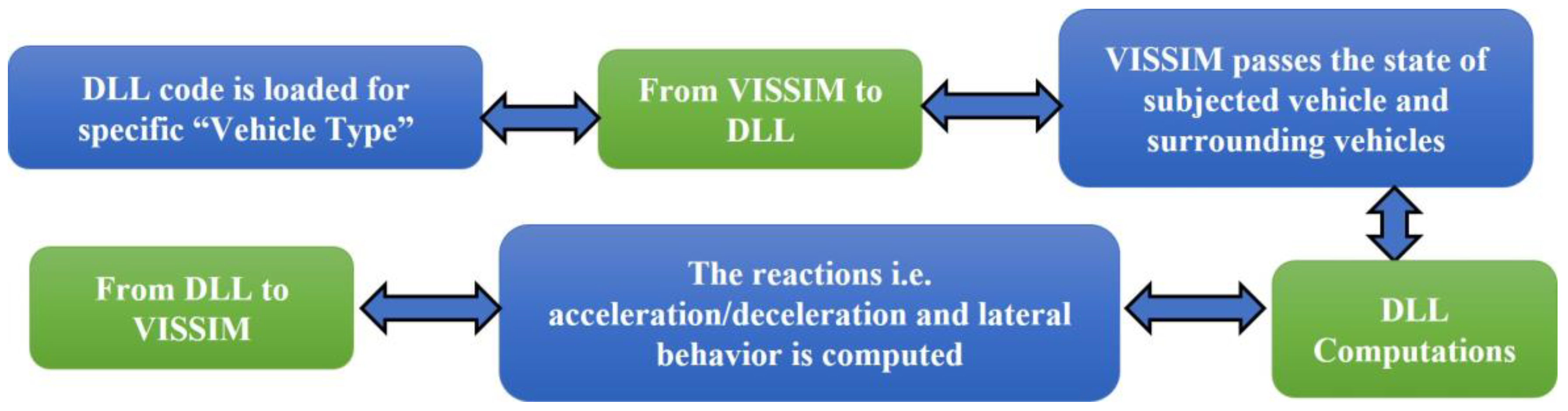
3.1. Integration of CACC and CACF Driving Models in VISSIM
3.2. Safety Performance Analysis Configuration
3.3. Simulation Configurations for Evaluation
4. Test Setup
4.1. Test 1–Maximum Throughput for CACF Model
4.2. Test 2—Performance of CACC and CACF Models (No-Crash)
4.3. Test 3—Performance of CACC and CACF Models (With-Crash)
4.4. Test 4—Impact of Acceleration Coefficients on CACF Model (With-Crash)
4.5. Test 5—Impact of V2I Communication Range on CACF Model (With-Crash)
4.6. Test 6—Impact of Communication Signal Lag on CACF Model (With-Crash)
- Case-1 for 0.1 s lag = = 0.6 s.
- Case-2 for 0.2 s lag = = 0.7 s.
- Case-3 for 0.3 s lag = = 0.8 s.
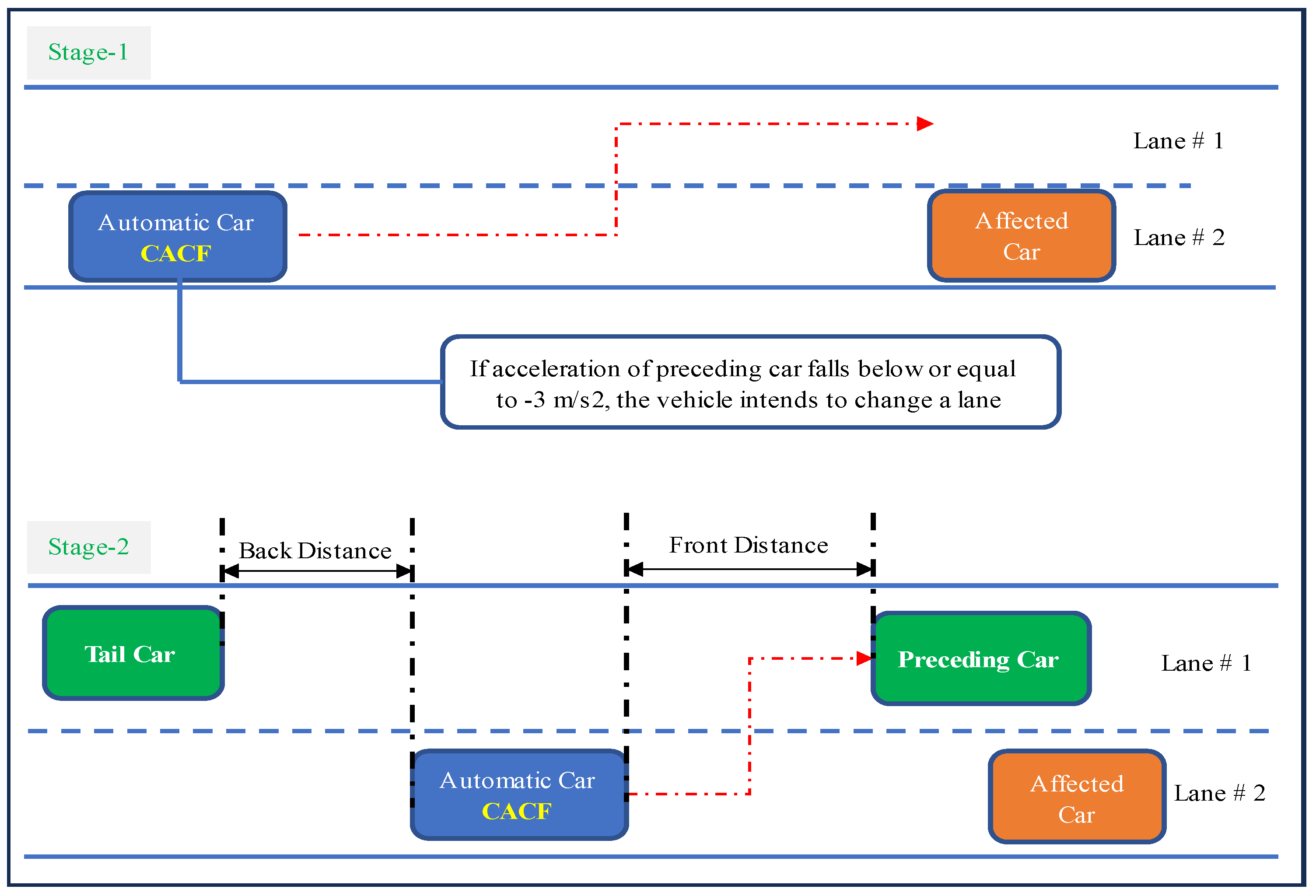
4.7. Test 7—Safety Perfromane of CACF Multi-Lane Logic
5. Results and Discussion
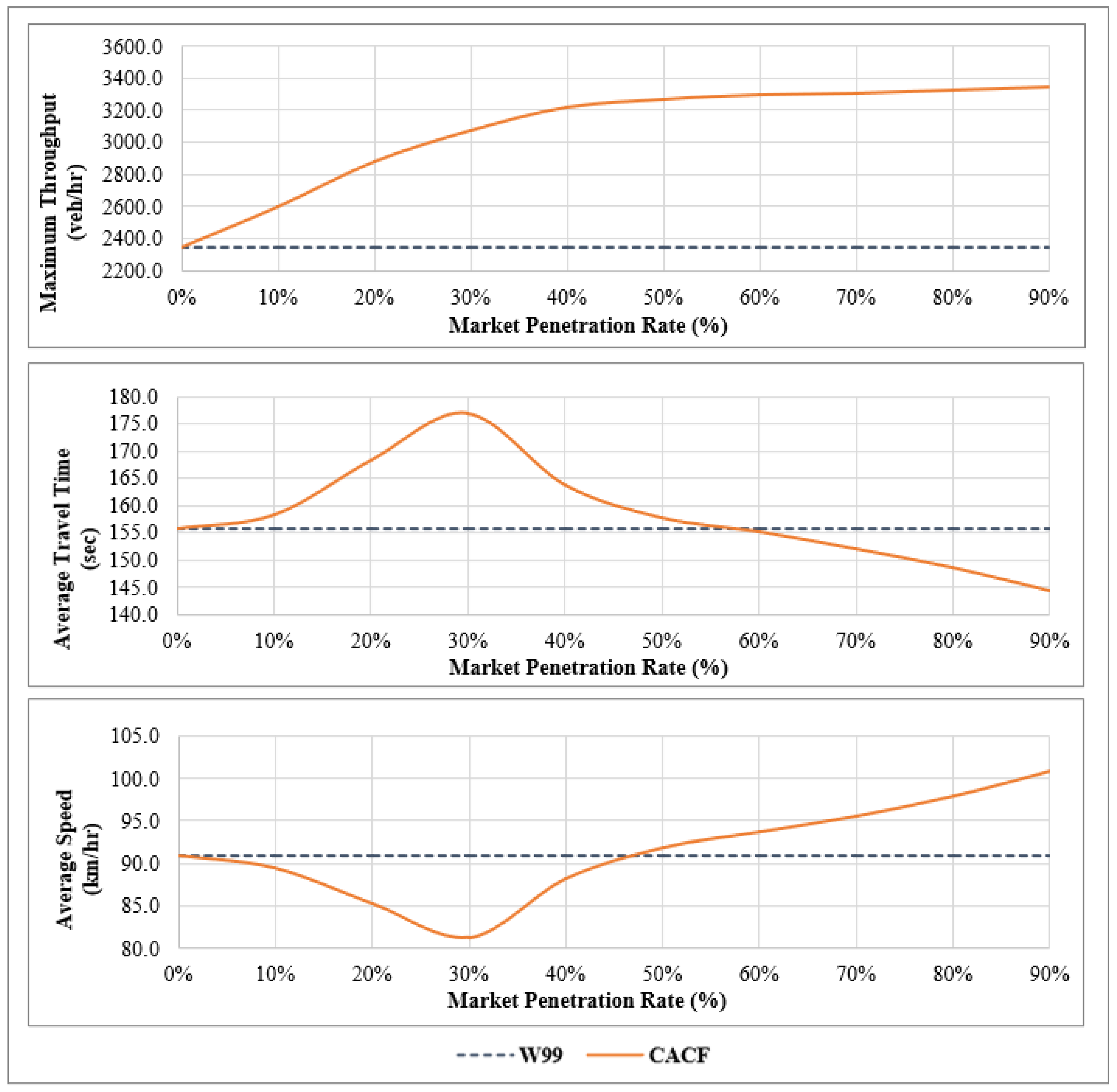
5.1. Test 1—Maximum Throughput for CACF Model
5.2. Test 2—Performance of CACC and CACF Models (No-Crash)
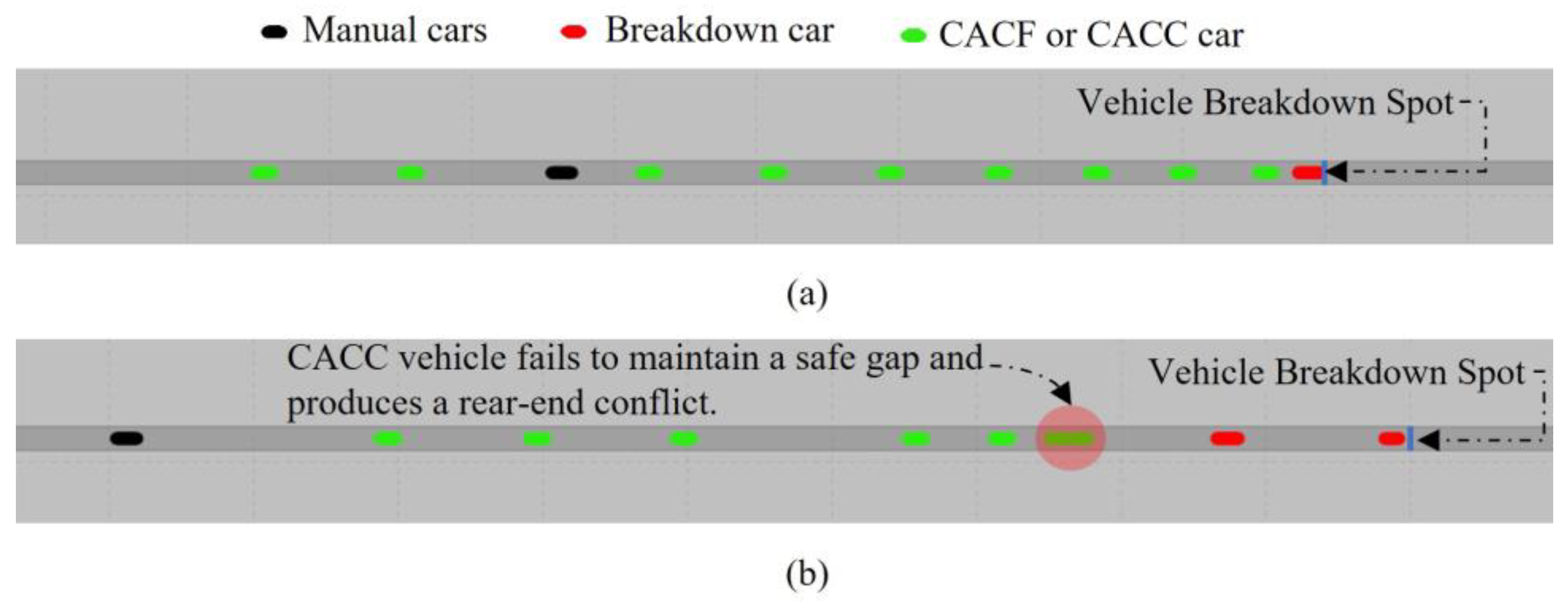
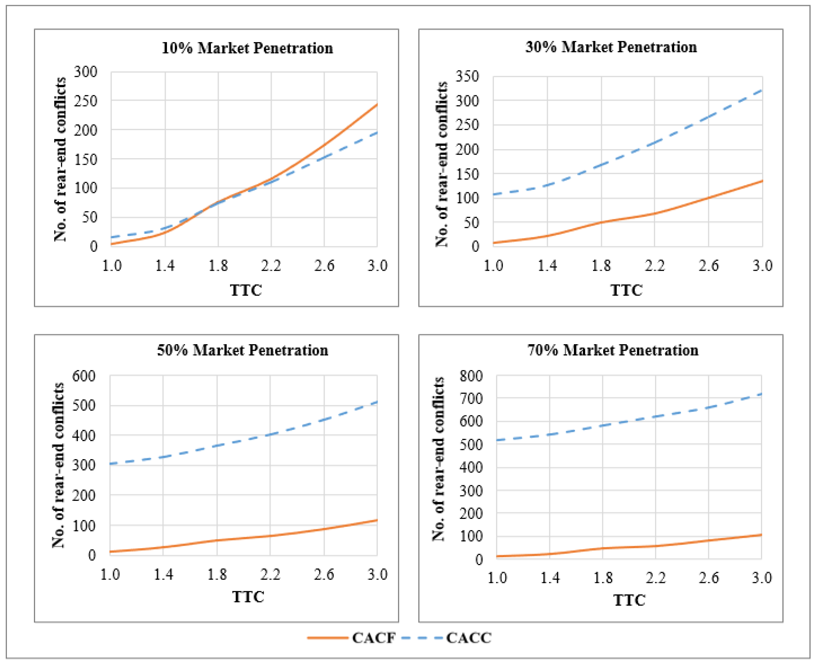
5.3. Test 3—Performance of CACC and CACF Models (With-Crash)
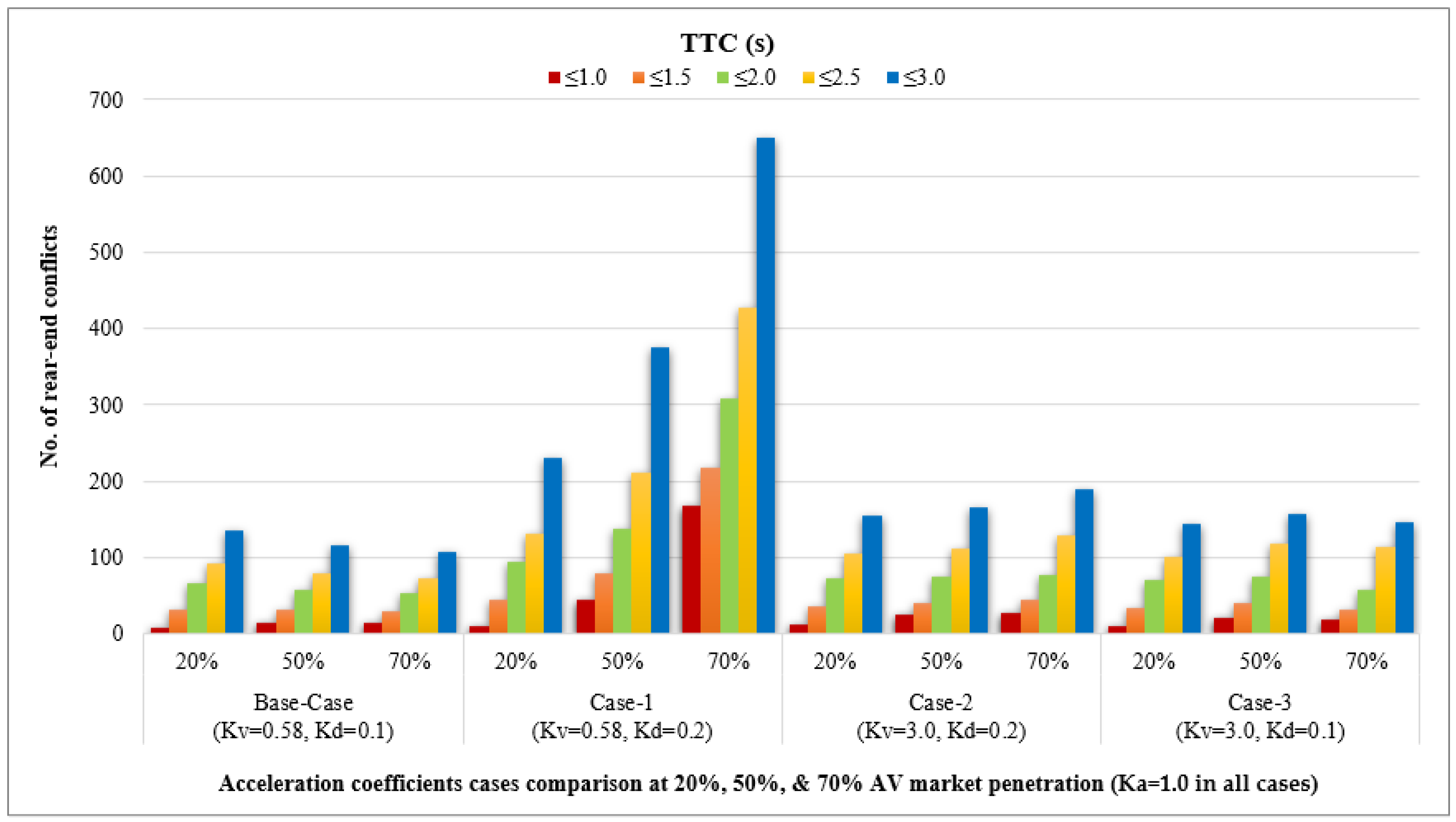
5.4. Test 4—Impact of Acceleration Coefficients on CACF Model (With-Crash)
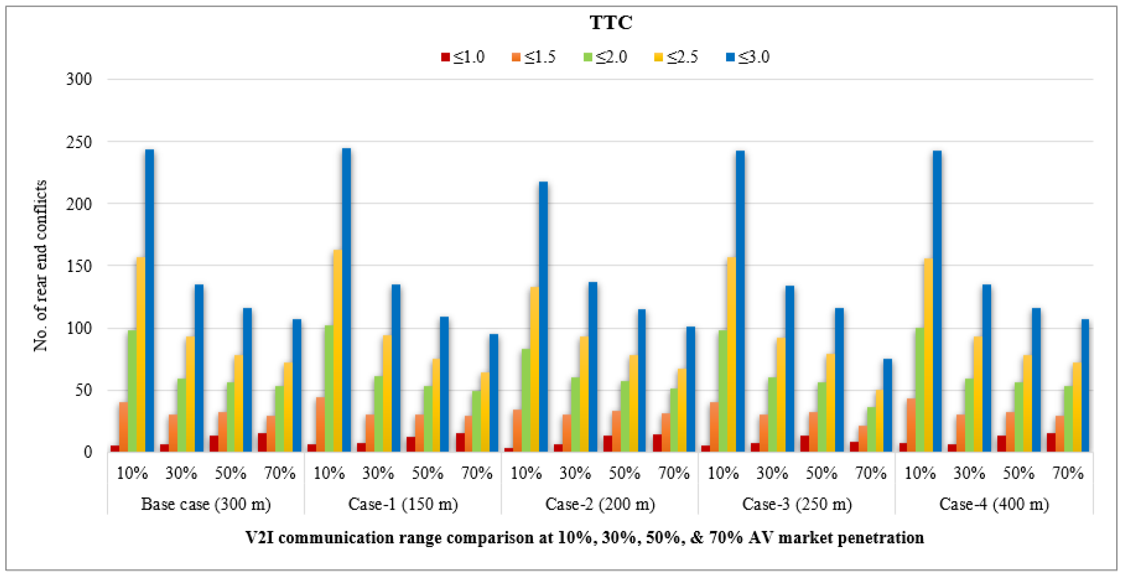
5.5. Test 5—Impact of V2I Communication Range on CACF Model (With-Crash)
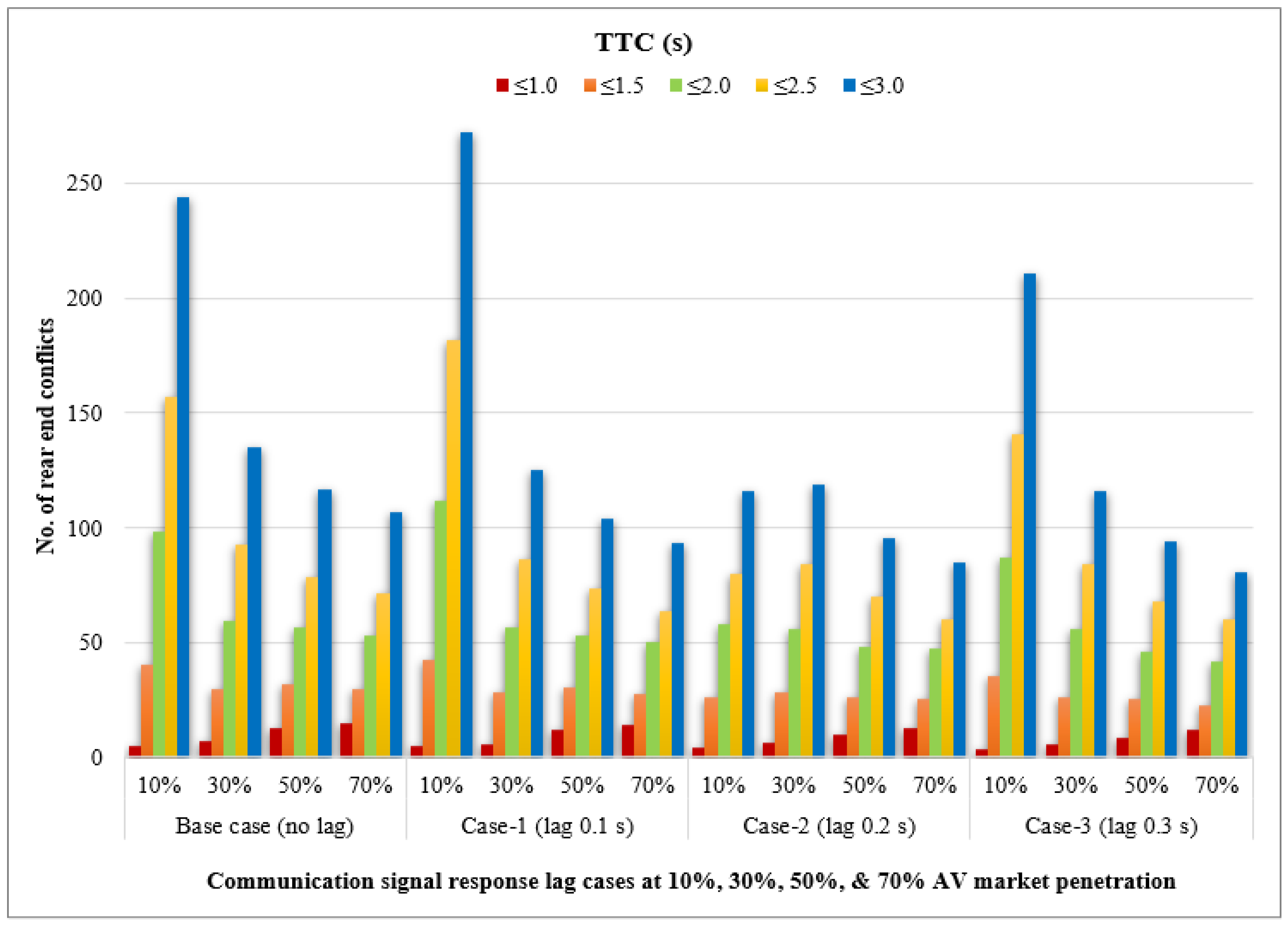
5.6. Test 6—Impact of Communication Signal Lag on CACF Model (With-Crash)
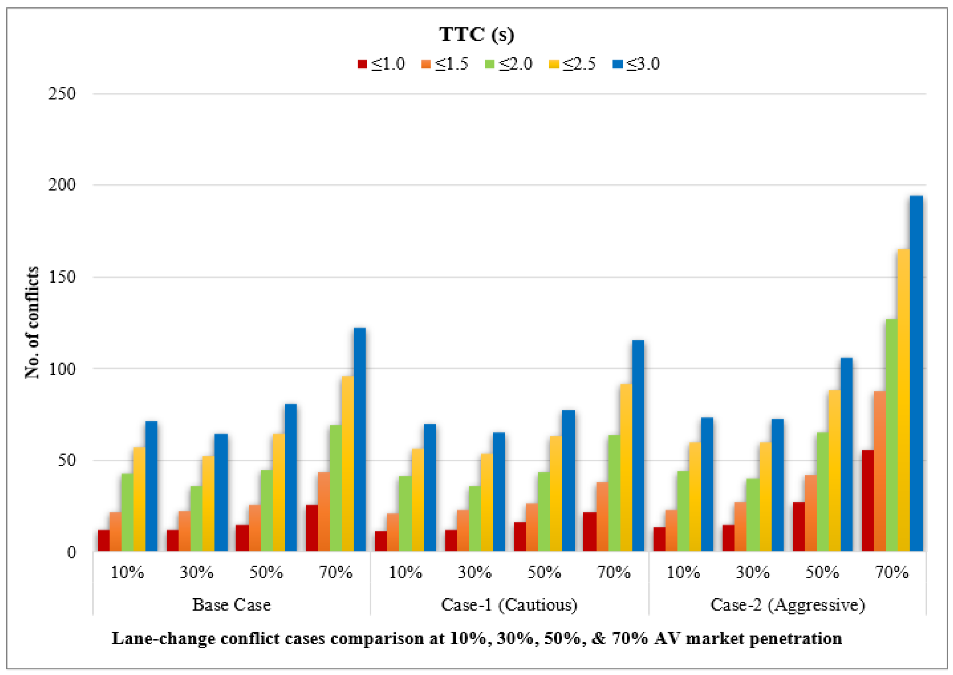
5.7. Test 7—Safety Performance of CACF Multi-Lane Logic
5.8. Discussion
6. Conclusions and Recommendations
- (1)
- For the maximum throughput test, it is observed that, with the increase in penetration rates, the CACF can significantly improve traffic capacity up to 42%. The test results for mobility performance for CACC and CACF have shown a drastic reduction in traffic delays at the progressive implementation of the driving logic. However, the CACF mobility benefits are further enhanced, as evident compared to CACC. Additionally, the CACF model avoids aggressive braking and traffic shockwaves, which are created by a breakdown vehicle due to cumulative-anticipative communication with the preceding vehicle. However, the inclusion of signal response delay negatively impacted the acceleration of AVs, and the vehicle maintains a “careful” behaviour.
- (2)
- For the safety analysis of the single-lane segment, the CACC model only performs better at a 10% market penetration rate. In contrast, the CACF model drastically improves network safety by reducing the number of rear-end conflicts with the increasing market penetration rates of CAVs. It is observed that the acceleration coefficient of distance Kd exerts the most influence on the network safety, as the number of conflicts increases for higher Kd values. The communication range of 200–250 m is found suitable for the CACF model, and the inclusion of signal response delay also resulted in the reduction of traffic conflicts. Furthermore, the results for CACF multi-lane logic show significant improvement in traffic safety because it considers both lateral and longitudinal communication for connected vehicles. However, it is only possible when an adequate distance is available in the adjacent lane.
- (3)
- This study recommends adopting the CACF car-following technique for future research, particularly in the context of V2I technology integration. This approach holds the potential to address prevalent challenges related to road safety, traffic delays, and travel costs. While the advantages of V2V technology become feasible with higher market penetration of AVs and CAVs, it is crucial to acknowledge that not all vehicles will be equipped with connected vehicle technology in the near future. Gathering characteristics and data for each vehicle within the communication range could be a challenging task. Therefore, early investments in V2I technology would pave the way for safe and convenient mobility solutions.
- (4)
- Improving the safety of CACC logic during accidents involves enhancing the ego car’s communication capabilities, employing a multi-anticipative technique. Effective communication with the environment allows the car to make informed decisions. Forming platoons is expected to positively impact road safety. Establishing criteria for “emergency braking”, with an aggressive deceleration value like −9.9 m/s2, can further mitigate rear-end conflicts.
Author Contributions
Funding
Data Availability Statement
Conflicts of Interest
Abbreviations
| ACC | Adaptive Cruise Control |
| API | Application Programming Interface |
| ASCE | American Society of Civil Engineers |
| AV | Autonomous Vehicle |
| CACC | Cooperative Adaptive Cruise Control |
| CACF | Cumulative-Anticipative Car-Following |
| CAV | Connected Autonomous Vehicle |
| DLL | Dynamic Library |
| EDM | External Driver Model |
| FHWA | Federal Highway Authority |
| FVD | Full Velocity Difference |
| HCM | Highway Capacity Manual |
| IDM | Intelligent Driver Model |
| ITS | Intelligent Transportation System |
| LDW | Lane Departure Warning |
| LOS | Level of Service |
| MassDOT | Massachusetts Department of Transportation |
| MOE | Measures of Effectiveness |
| NHTSA | National Highway Traffic Safety Administration |
| ODOT | Oregon Department of Transportation |
| PET | Post-encroachment-time |
| SSAM | Safety Surrogate Assessment Model |
| TTC | Time-to-collision |
| V2I | Vehicle-to-Infrastructure |
| V2V | Vehicle-to-vehicle |
| V2X | Vehicle-to-everything |
| W99 | Wiedemann 99 |
| WSDOT | Washington State Department of Transportation |
References
- NHTSA. Early Estimate of Motor Vehicle Traffic Fatalities in 2020; United States Department of Transportation: Washington, DC, USA, 2022.
- WHO. Global Status Report on Road Safety 2015; World Health Organization: Geneva, Switzerland, 2015. [Google Scholar]
- American Society of Civil Engineers (ASCE). 2021 Infrastructure Report Card; American Society of Civil Engineers: Reston, VA, USA, 2021. [Google Scholar]
- Litman, T. Autonomous Vehicle Implementation Predictions; Victoria Transport Policy Institute: Victoria, BC, Canada, 2017. [Google Scholar]
- NHTSA. National Motor Vehicle Crash Causation Survey: Report to Congres; National Highway Traffic Safety Administration Technical Report DOT HS; NHTSA: Washington DC, USA, 2008; Volume 811, p. 59.
- Greenblatt, N.A. Self-driving cars and the law. IEEE Spectr. 2016, 53, 46–51. [Google Scholar] [CrossRef]
- Shanker, R. Autonomous Cars: Self-Driving the New Auto Industry Paradigm; Morgan Stanley Blue Paper; Morgan Stanley: New York, NY, USA, 2013; pp. 1–109. [Google Scholar]
- Leech, J.; Whelan, G.; Bhaiji, M.; Hawes, M.; Scharring, K. Connected and Autonomous Vehicles—The UK Economic Opportunity. KPMG. 2015, Volume 80. Available online: https://www.smmt.co.uk/wp-content/uploads/sites/2/CRT036586F-Connected-and-Autonomous-Vehicles-%E2 (accessed on 1 February 2021).
- Dennis, E.P.; Spulber, A.; Sathe Brugerman, V.; Kuntzsch, R.; Neuner, R. Planning for Connected and Automated Vehicles. Technology Research; Center for Automotive Research: Ann Arbor, MI, USA, 2017; Available online: https://www.cargroup.org/publication/planning-for-connected-and-automated-vehicles/ (accessed on 1 February 2021).
- Hars, A. Autonomous cars: The next revolution looms. Inven. Innov. Briefs 2010, 1, 2010. [Google Scholar]
- Talebpour, A.; Mahmassani, H.S. Influence of connected and autonomous vehicles on traffic flow stability and throughput. Transp. Res. Part C Emerg. Technol. 2016, 71, 143–163. [Google Scholar] [CrossRef]
- Mervis, J. Are We Going Too Fast on Driverless Cars. Science. 12 December 2017. Available online: https://www.science.org/content/article/are-we-going-too-fast-driverless-cars (accessed on 1 February 2021).
- Simonite, T. Prepare to be underwhelmed by 2021’s autonomous cars. MIT Technol. Rev. 2016. Available online: https://www.technologyreview.com/2016/08/23/157929/prepare-to-be-underwhelmed-by-2021s-autonomous-cars/ (accessed on 1 February 2021).
- Chen, S.; Hu, J.; Shi, Y.; Peng, Y.; Fang, J.; Zhao, R.; Zhao, L. Vehicle-to-everything (V2X) services supported by LTE-based systems and 5G. IEEE Commun. Stand. Mag. 2017, 1, 70–76. [Google Scholar] [CrossRef]
- Gupta, M.; Benson, J.; Patwa, F.; Sandhu, R. Secure V2V and V2I communication in intelligent transportation using cloudlets. IEEE Transp. Serv. Comput. 2020, 15, 1912–1925. [Google Scholar] [CrossRef]
- Milanés, V.; Villagrá, J.; Godoy, J.; Simó, J.; Pérez, J.; Onieva, E. An intelligent V2I-based traffic management system. IEEE Trans. Intell. Transp. Syst. 2012, 13, 49–58. [Google Scholar] [CrossRef]
- Bagheri, M.; Siekkinen, M.; Nurminen, J.K. Cellular-based vehicle to pedestrian (V2P) adaptive communication for collision avoidance. In Proceedings of the 2014 International Conference on Connected Vehicles and Expo (ICCVE), Vienna, Austria, 3–7 November 2014; IEEE: Washington, DC, USA, 2014; pp. 450–456. [Google Scholar]
- Saeed, U.; Hämäläinen, J.; Mutafungwa, E.; Wichman, R.; González, D.; Garcia-Lozano, M. Route-based radio coverage analysis of cellular network deployments for V2N communication. In Proceedings of the 2019 International Conference on Wireless and Mobile Computing, Networking and Communications (WiMob), Barcelona, Spain, 21–23 October 2019; IEEE: Washington, DC, USA, 2019; pp. 1–6. [Google Scholar]
- Ahmed, H.U.; Huang, Y.; Lu, P. A review of car-following models and modeling tools for human and autonomous-ready driving behaviors in micro-simulation. Smart Cities 2021, 4, 314–335. [Google Scholar] [CrossRef]
- Yang, X.; Ahemd, H.U.; Huang, Y.; Lu, P. Cumulatively Anticipative Car-Following Model with Enhanced Safety for Autonomous Vehicles in Mixed Driver Environments. Smart Cities 2023, 6, 2260–2281. [Google Scholar] [CrossRef]
- Tettamanti, T.; Varga, I.; Szalay, Z. Impacts of autonomous cars from a traffic engineering perspective. Period. Polytech. Transp. Eng. 2016, 44, 244–250. [Google Scholar] [CrossRef]
- Sukennik, P.; Lohmiller, J.; Schlaich, J. Simulation-based forecasting the impacts of autonomous driving. In Proceedings of the International Symposium of Transport Simulation (ISTS’18) and the International Workshop on Traffic Data Collection and its Standardization (IWTDCS’18), Matsuyama, Japan, 4–6 August 2018; pp. 6–8. [Google Scholar]
- Songchitruksa, P.; Bibeka, A.; Lin, L.I.; Zhang, Y. Incorporating Driver Behaviors into Connected and Automated Vehicle Simulation; Center for Advancing Transportation Leadership and Safety (ATLAS Center): New York, NY, USA, 2016. [Google Scholar]
- Seraj, M.; Li, J.; Qiu, Z. Modeling microscopic car-following strategy of mixed traffic to identify optimal platoon configurations for multiobjective decision-making. J. Adv. Transp. 2018, 2018, 7835010. [Google Scholar] [CrossRef]
- ATKINS. Research on the Impacts of Connected and Autonomous Vehicles (CAVs) on Traffic Flow, Stage 2: Traffic Modelling and Analysis; Technical Report; Department for Transport, ATKINS: London, UK, 2016. [Google Scholar]
- Kotsialos, A.; Papageorgiou, M.; Diakaki, C.; Pavlis, Y.; Middelham, F. Traffic flow modeling of large-scale motorway networks using the macroscopic modeling tool METANET. IEEE Trans. Intell. Transp. Syst. 2002, 3, 282–292. [Google Scholar] [CrossRef]
- Lu, X.-Y.; Qiu, T.Z.; Varaiya, P.; Horowitz, R.; Shladover, S.E. Combining variable speed limits with ramp metering for freeway traffic control. In Proceedings of the 2010 american control conference, Baltimore, MD, USA, 30 June–2 July 2010; IEEE: Washington, DC, USA, 2010; pp. 2266–2271. [Google Scholar]
- FHWA. Types of Traffic Analysis Tools. 2023. Available online: https://ops.fhwa.dot.gov/trafficanalysistools/type_tools.htm (accessed on 1 February 2021).
- Olstam, J.J.; Tapani, A. Comparison of Car-Following Models; Swedish National Road and Transport Research Institute: Linköping, Sweden, 2004; Volume 960.
- Hoogendoorn, S.P.; Hoogendoorn, R. Generic calibration framework for joint estimation of car-following models by using microscopic data. Transp. Res. Rec. 2010, 2188, 37–45. [Google Scholar] [CrossRef]
- Lochrane, T. A New Multidimensional Psycho-Physical Framework for Modeling Car-Following in a Freeway Work Zone. Ph.D. Thesis, University of Central Florida, Orlando, FL, USA, 2014. [Google Scholar]
- Jones, S.L.; Sullivan, A.J.; Cheekoti, N.; Anderson, M.D.; Malave, D. Traffic simulation software comparison study. UTCA Rep. 2004, 2217, 58. [Google Scholar]
- PTV, A.G. VISSIM 2020.00 User Manual; PTV Karlsruhe: Karlsruhe, Germany, 2020. [Google Scholar]
- Gipps, P.G. A model for the structure of lane-changing decisions. Transp. Res. Part B Methodol. 1986, 20, 403–414. [Google Scholar] [CrossRef]
- Sparmann, U. Spurwechselvorgänge auf zweispurigen BAB-Richtungsfahrbahnen; Forsch Strassenbau u Strassenverkehrstech 263; No. 263; Forschungsgesellschaft für Straßen- und Verkehrswesen (FGSV): Berling, Germany, 1978. [Google Scholar]
- Pipes, L.A. An operational analysis of traffic dynamics. J. Appl. Phys. 1953, 24, 274–281. [Google Scholar] [CrossRef]
- Gazis, D.C.; Herman, R.; Rothery, R.W. Nonlinear follow-the-leader models of traffic flow. Oper. Res. 1961, 9, 545–567. [Google Scholar] [CrossRef]
- Toledo, T.; Koutsopoulos, H.N.; Ben-Akiva, M. Integrated driving behavior modeling. Transp. Res. Part C Emerg. Technol. 2007, 15, 96–112. [Google Scholar] [CrossRef]
- Gipps, P.G. A behavioural car-following model for computer simulation. Transp. Res. Part B Methodol. 1981, 15, 105–111. [Google Scholar] [CrossRef]
- Bando, M.; Hasebe, K.; Nakayama, A.; Shibata, A.; Sugiyama, Y. Dynamical model of traffic congestion and numerical simulation. Phys. Rev. E 1995, 51, 1035. [Google Scholar] [CrossRef]
- Wiedemann, R.; Reiter, U. Microscopic Traffic Simulation: The Simulation System MISSION, Background and Actual State; Project ICARUS (V1052) Final Report; CEC: Brussels, Belgium, 1992; Volume 2, pp. 1–53. [Google Scholar]
- Saifuzzaman, M.; Zheng, Z. Incorporating human-factors in car-following models: A review of recent developments and research needs. Transp. Res. Part C Emerg. Technol. 2014, 48, 379–403. [Google Scholar] [CrossRef]
- Sun, L.; Jafaripournimchahi, A.; Kornhauser, A.; Hu, W. A new higher-order viscous continuum traffic flow model considering driver memory in the era of autonomous and connected vehicles. Phys. A Stat. Mech. Its Appl. 2020, 547, 123829. [Google Scholar] [CrossRef]
- Jafaripournimchahi, A.; Sun, L.; Hu, W. Driver’s anticipation and memory driving car-following model. J. Adv. Transp. 2020, 2020, 4343658. [Google Scholar] [CrossRef]
- Milanés, V.; Shladover, S.E. Modeling cooperative and autonomous adaptive cruise control dynamic responses using experimental data. Transp. Res. Part C Emerg. Technol. 2014, 48, 285–300. [Google Scholar] [CrossRef]
- Treiber, M.; Hennecke, A.; Helbing, D. Congested traffic states in empirical observations and microscopic simulations. Phys. Rev. E 2000, 62, 1805. [Google Scholar] [CrossRef]
- Kockelman, K.M.; Avery, P.; Bansal, P.; Boyles, S.D.; Bujanovic, P.; Choudhary, T.; Clements, L.; Domnenko, G.; Fagnant, D.; Helsel, J.; et al. Implications of Connected and Automated Vehicles on the Safety and Operations of Roadway Networks: A Final Report; The University of Texas: Austin, TX, USA, 2016. [Google Scholar]
- Van Arem, B.; Van Driel, C.J.G.; Visser, R. The impact of cooperative adaptive cruise control on traffic-flow characteristics. IEEE Trans. Intell. Transp. Syst. 2006, 7, 429–436. [Google Scholar] [CrossRef]
- Dey, K.C.; Yan, L.; Wang, X.; Wang, Y.; Shen, H.; Chowdhury, M.; Yu, L.; Qiu, C.; Soundararaj, V. A review of communication, driver characteristics, and controls aspects of cooperative adaptive cruise control (CACC). IEEE Trans. Intell. Transp. Syst. 2015, 17, 491–509. [Google Scholar] [CrossRef]
- Werf, J.V.; Shladover, S.E.; Miller, M.A.; Kourjanskaia, N. Effects of adaptive cruise control systems on highway traffic flow capacity. Transp. Res. Rec. 2002, 1800, 78–84. [Google Scholar] [CrossRef]
- Shladover, S.E.; Su, D.; Lu, X.-Y. Impacts of cooperative adaptive cruise control on freeway traffic flow. Transp. Res. Rec. 2012, 2324, 63–70. [Google Scholar] [CrossRef]
- Schermers, G.; Malone, K.M.; van Arem, B. Dutch evaluation of chauffeur assistant traffic flow effects on implementation in the heavy goods vehicle sector. In Proceedings of the 11th World Congress on Intelligent Transport Systems, ITS 2004: ITS for Livable Society (World Congress on Intelligent Transport Systems), Nagoya, Japan, 18–24 October 2004. [Google Scholar]
- Van Arem, B.; De Vos, A.P.; Vanderschuren, M.J.W.A. The Microscopic Traffic Simulation Model MIXIC 1.3. 1997. Available online: https://trid.trb.org/view/634929 (accessed on 1 February 2021).
- Hunter, M.P.; Guin, A.; Rodgers, M.O.; Huang, Z.; Greenwood, A.T. Cooperative Vehicle–Highway Automation (CVHA) Technology: Simulation of Benefits and Operational Issues; Federal Highway Administration: Washington, DC, USA, 2017.
- Hidas, P. Modelling lane changing and merging in microscopic traffic simulation. Transp. Res. Part C Emerg. Technol. 2002, 10, 351–371. [Google Scholar] [CrossRef]
- Liu, J.; Kockelman, K.; Nichols, A. Anticipating the emissions impacts of smoother driving by connected and autonomous vehicles, using the MOVES model. In Proceedings of the Transportation Research Board 96th Annual Meeting, Washington, DC, USA, 8–12 January 2017. [Google Scholar]
- Zhao, L.; Sun, J. Simulation framework for vehicle platooning and car-following behaviors under connected-vehicle environment. Procedia-Soc. Behav. Sci. 2013, 96, 914–924. [Google Scholar] [CrossRef]
- Xiaorui, W.; Hongxu, Y. A lane change model with the consideration of car following behavior. Procedia-Soc. Behav. Sci. 2013, 96, 2354–2361. [Google Scholar] [CrossRef]
- Vechione, M.; Balal, E.; Cheu, R.L. Comparisons of mandatory and discretionary lane changing behavior on freeways. Int. J. Transp. Sci. Technol. 2018, 7, 124–136. [Google Scholar] [CrossRef]
- Gettman, D.; Pu, L.; Sayed, T.; Shelby, S.G.; Energy, S. Surrogate Safety Assessment Model and Validation; Turner-Fairbank Highway Research Center: McLean, VA, USA, 2008. [Google Scholar]
- Miqdady, T.; de Oña, R.; Casas, J.; de Oña, J. Studying traffic safety during the transition period between manual driving and autonomous driving: A simulation-based approach. IEEE Trans. Intell. Transp. Syst. 2023, 24, 6690–6710. [Google Scholar] [CrossRef]
- Miqdady, T.; de Oña, R.; de Oña, J. Traffic Safety Sensitivity Analysis of Parameters Used for Connected and Autonomous Vehicle Calibration. Sustainability 2023, 15, 9990. [Google Scholar] [CrossRef]
- Hayward, J.C. Near Miss Determination through Use of a Scale of Danger. 1972. Available online: https://onlinepubs.trb.org/Onlinepubs/hrr/1972/384/384-004.pdf (accessed on 1 February 2021).
- Sayed, T.; Brown, G.; Navin, F. Simulation of traffic conflicts at unsignalized intersections with TSC-Sim. Accid. Anal. Prev. 1994, 26, 593–607. [Google Scholar] [CrossRef]
- Hydén, C.; Linderholm, L. The Swedish Traffic-Conflicts Technique. In International Calibration Study of Traffic Conflict Techniques; Springer: Berlin/Heidelberg, Germany, 1984; pp. 133–139. [Google Scholar]
- MassDOT. MassDOT Guidelines for Calibrating Roundabouts in VISSIM Simulation Models. 2020. Available online: https://www.mass.gov/doc/massdot-roundabout-vissim-microsimulation-guidance/download (accessed on 1 January 2024).
- Oregon DOT. Protocol for VISSIM Simulation. Available online: www.oregon.gov/odot/td/tp/apm/addc.pdf (accessed on 1 February 2021).
- Schilperoort, L.; McClanahan, D.; Shank, R.; Bjordahl, M. Protocol for VISSIM Simulation; Washington State Department of Transportation: Washington, DC, USA, 2014.
- Dowling, R.; Skabardonis, A.; Alexiadis, V. Traffic Analysis Toolbox, Volume III: Guidelines for Applying Traffic Microsimulation Modeling Software; United States Federal Highway Administration, Office of Operations: Washington, DC, USA, 2004.
- Harding, J.; Powell, G.; Yoon, R.; Fikentscher, J.; Doyle, C.; Sade, D.; Lukuc, M.; Simons, J.; Wang, J. Vehicle-to-Vehicle Communications: Readiness of V2V Technology for Application; National Highway Traffic Safety Administration: Washington, DC, USA, 2014.
- Manual, H.C. Highway Capacity Manual; Transportation Research Board: Washington, DC, USA, 2000; Volume 2. [Google Scholar]


| Scenario | Average Delay | Average Journey Time | ||
|---|---|---|---|---|
| (s) | (%) | (s) | (%) | |
| Base | 35.84 | - | 539.79 | - |
| 25% CAV | 36.17 | +0.9 | 538.49 | −0.2 |
| 50% CAV | 33.39 | −6.8 | 533.62 | −1.1 |
| 75% CAV | 29.77 | −16.9 | 527.72 | −2.2 |
| 100% CAV | 23.72 | −33.8 | 517.77 | −4.1 |
| Upper bound * | 21.38 | −40.3 | 479.29 | −11.2 |
| Slower lane-change | 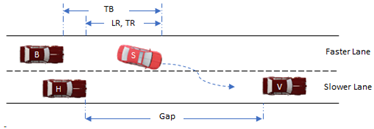 |
| Type-1: FREE lane-changes | 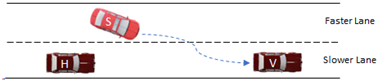 |
| Type-2: ACCEL lane-changes |  |
| Faster lane-changes |  |
| Type-1: FREE lane-changes | 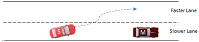 |
| Type-2: LEAD lane-changes | 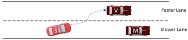 |
| Type-3: LAG lane-changes | 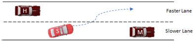 |
| Type-4: GAP lane-changes | 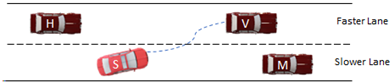 |
| Type of Test Setup | Type of Analysis | |
|---|---|---|
| Mobility | Safety | |
| Test 1—Maximum Throughput for CACF Model | ✓ | |
| Test 2—Performance of CACC and CACF Models (No-Crash) | ✓ | |
| Test 3—Performance of CACC and CACF Models (With-Crash) | ✓ | ✓ |
| Test 4—Impact of Acceleration Coefficients on CACF Model (With-Crash) | ✓ | |
| Test 5—Impact of V2I Communication Range on CACF Model (With-Crash) | ✓ | |
| Test 6—Impact of Communication Signal Lag on CACF Model (With-Crash) | ✓ | ✓ |
| Test 7—Safety Performance of CACF Multi-lane Logic | ✓ | |
| Coefficient Comparison Cases | Coefficient Values | ||
|---|---|---|---|
| Ka | Kv | Kd | |
| Base-case | 1.0 | 0.58 | 0.1 |
| Case-1 | 1.0 | 0.58 | 0.2 |
| Case-2 | 1.0 | 3.0 | 0.2 |
| Case-3 | 1.0 | 3.0 | 0.1 |
| Cases for Different Communication Ranges | Values (m) | Capability for Communication with “n” Number of Cars 1 | No. of Cars (#) |
|---|---|---|---|
| Base Case | 300 | Base Case | 10 |
| Case-1 | 150 | Case-1 | 5 |
| Case-2 | 200 | Case-2 | 15 |
| Case-3 | 250 | ||
| Case-4 | 400 |
| Market Penetration (%) | Average Travel Time (s) | Average Delay (s) | Average Speed (km/h) | ||||||
|---|---|---|---|---|---|---|---|---|---|
| W99 | CACF | CACC | W99 | CACF | CACC | W99 | CACF | CACC | |
| 0 | 148.9 | - | - | 13.9 | - | - | 97.6 | - | - |
| 30 | - | 146.7 | 147.2 | - | 10.2 | 8.8 | - | 99.2 | 98.6 |
| 50 | - | 145 | 145.3 | - | 7.3 | 5.6 | - | 100.6 | 99.8 |
| 70 | - | 142.4 | 142.5 | - | 3.3 | 2.7 | - | 102.9 | 101.7 |
| 90 | - | 135.9 | 139.4 | - | −5.3 1 | 0.6 | - | 108.9 | 103.9 |
| Market Penetration (%) | Average Travel Time (s) | Average Delay (s) | Average Speed (km/h) | ||||||
|---|---|---|---|---|---|---|---|---|---|
| W99 | CACF | CACC | W99 | CACF | CACC | W99 | CACF | CACC | |
| 0 | 150.2 | - | - | 14.9 | - | - | 96.9 | - | - |
| 30 | - | 147.6 | 148.8 | - | 10.9 | 8.0 | - | 98.7 | 97.7 |
| 50 | - | 146.2 | 147.5 | - | 8.3 | 5.7 | - | 100 | 98.6 |
| 70 | - | 143.7 | 144.7 | - | 4.4 | 3.5 | - | 102.2 | 100.5 |
| 90 | - | 138.4 | 141.3 | - | −3.2 1 | 1.1 | - | 107.2 | 102.8 |
| Market Penetration (%) | Average Delay (s) | |||
|---|---|---|---|---|
| Base Case | Case 1 0.1 s lag | Case 2 0.2 s lag | Case 3 0.3 s lag | |
| 10 | 13.5 | 13.6 | 13.6 | 13.7 |
| 30 | 10.9 | 11.1 | 11.1 | 11.3 |
| 50 | 8.3 | 8.4 | 8.6 | 8.9 |
| 70 | 4.4 | 4.7 | 5 | 5.3 |
| Tests | Mobility 1 | Safety 1 |
|---|---|---|
| Test 1—Maximum throughput for CACF model | The road capacity for the CACF model increases by 35% for a 90% market penetration compared to the VISSIM default Wiedemann 99 car-following model. | - |
| Test 2—Performance of CACC and CACF models (no-crash) | The average delay of the Wiedemann 99 model is 13.9 s. However, the delay is drastically reduced to 0.0 s and 0.6 s for CACF and CACC models, respectively, at a 90% market penetration rate. | |
| Test 3—Performance of CACC and CACF models (with-crash) | The mobility performance of both models has low significance. | The CACC model only performs better at a 10% market penetration rate. The CACF model drastically improves network safety for increasing market penetration rates. |
| Test 4—Impact of acceleration coefficients on CACF model (with-crash) | - | The acceleration coefficient of distance “Kd” is most influential to network safety. The number of conflicts increases for higher “Kd” values. |
| Test 5—Impact of V2I communication range on CACF model (with-crash) | A communication range between 200 to 250 m is suitable for the CACF model. | |
| Test 6—Impact of communication signal lag on CACF model (with-crash) | Because the vehicle begins to move with slower acceleration, average delay starts to increase. The increase in average delay is recorded to be only 0.9 s between base case and Case 3, at a 70% market penetration rate. | The inclusion of signal response lag negatively impacts the acceleration of automatic vehicles, and the vehicle maintains a “careful” behaviour. For TTC ≤ 3.0 at a 50% market penetration rate, average conflicts are reduced by approximately 11% for 0.1 s lag, 20% for 0.2 s lag, and 21% for 0.3 s lag. |
| Test 7—Safety performance of CACF multi-lane logic | - | The CACF cautious lane-change and VISSIM default lane-change performs safer compared to the CACF aggressive model. |
Disclaimer/Publisher’s Note: The statements, opinions and data contained in all publications are solely those of the individual author(s) and contributor(s) and not of MDPI and/or the editor(s). MDPI and/or the editor(s) disclaim responsibility for any injury to people or property resulting from any ideas, methods, instructions or products referred to in the content. |
© 2024 by the authors. Licensee MDPI, Basel, Switzerland. This article is an open access article distributed under the terms and conditions of the Creative Commons Attribution (CC BY) license (https://creativecommons.org/licenses/by/4.0/).
Share and Cite
Ahmed, H.U.; Ahmad, S.; Yang, X.; Lu, P.; Huang, Y. Safety and Mobility Evaluation of Cumulative-Anticipative Car-Following Model for Connected Autonomous Vehicles. Smart Cities 2024, 7, 518-540. https://doi.org/10.3390/smartcities7010021
Ahmed HU, Ahmad S, Yang X, Lu P, Huang Y. Safety and Mobility Evaluation of Cumulative-Anticipative Car-Following Model for Connected Autonomous Vehicles. Smart Cities. 2024; 7(1):518-540. https://doi.org/10.3390/smartcities7010021
Chicago/Turabian StyleAhmed, Hafiz Usman, Salman Ahmad, Xinyi Yang, Pan Lu, and Ying Huang. 2024. "Safety and Mobility Evaluation of Cumulative-Anticipative Car-Following Model for Connected Autonomous Vehicles" Smart Cities 7, no. 1: 518-540. https://doi.org/10.3390/smartcities7010021
APA StyleAhmed, H. U., Ahmad, S., Yang, X., Lu, P., & Huang, Y. (2024). Safety and Mobility Evaluation of Cumulative-Anticipative Car-Following Model for Connected Autonomous Vehicles. Smart Cities, 7(1), 518-540. https://doi.org/10.3390/smartcities7010021