Optimizing Smart Campus Solutions: An Evidential Reasoning Decision Support Tool

Abstract

Smart technologies have become increasingly prevalent in various industries due to their potential for energy cost reduction, productivity gains, and sustainability. Smart campuses, which are educational institutions that implement smart technologies, have emerged as a specific application of these technologies. However, implementing available smart technologies is often not feasible due to various limitations, such as funding and cultural restrictions. In response, this study develops a mathematical decision-making tool based on the evidential reasoning (ER) approach and implemented in Python. The tool aims to assist universities in prioritizing smart campus solutions tailored to their specific needs. The research combines a comprehensive literature review with insights from stakeholder surveys to identify six principal objectives and four foundational technologies underpinning smart campus solutions. Additionally, six critical success factors and nine functional clusters of smart campus solutions are pinpointed, and evaluated through the ER approach. The developed decision-support tool underwent validation through various statistical tests and was found to be highly reliable, making it a generalized tool for worldwide use with different alternatives and attributes. The proposed tool provides universities with rankings and utilities to determine necessary smart applications based on inputs such as implementation cost, operation cost, maintenance cost, implementation duration, resource availability, and stakeholders’ perceived benefit.

1. Introduction

Smart cities are viewed as a necessary future development in response to global climate and ecological issues. However, not all of the available smart city technologies and frameworks are feasible or optimal [1]. As it would be expensive to replace an entire city’s infrastructure for experimentation purposes, it might be best to test smart applications on a smaller scale, such as a university campus [2]. Given that smart campuses have the potential to become models for future smart cities, as they emulate many aspects of cities within a limited area, but with fewer stakeholders and more control over assets, transforming traditional campuses into smart ones could contribute to the strategic development of the education sector and enhance its competitiveness. As such, universities, which typically host various functions within their campuses, are in a unique position to experiment with cutting-edge technologies, making them excellent testing grounds for different smart solutions [3]. By doing so, campuses can help to improve the socio-ecological aspects of their surrounding areas and contribute to the progress of their communities, regions, and cities [2].

According to [4], the increased accessibility of higher education across many countries and cultures has led to a significant growth in the number of students since the 1990s. Therefore, with the new innovative technologies and the reshaping of several aspects of human lives, educational institutions must develop and adapt to these new technologies and continue to innovate to meet the needs of a diverse student population. According to [5], such challenges present an opportunity for universities to experiment with different technologies to increase students’ comfort and satisfaction. Moreover, most new students were raised in a tech-driven, connected world [6], leading to high expectations for on-demand experiences and opportunities for investing in smart technologies for campus use.

In their work, Dong et al. [2] defined the term ‘smart’ as the ability to learn quickly, make intelligent judgments, and respond promptly to problems. They argue that a system can be considered smart when it can autonomously provide services that meet the dynamic needs of users. It is important to note that a smart campus goes beyond a smart application like a Chabot. A smart campus employs networked applications to promote collaboration, enhance resource efficiency, conserve resources, and ultimately create a more enjoyable environment for all.

Smart applications utilize recent information and communication technologies to manage smart buildings, territories, and businesses [7]. Within an educational environment, smart applications leverage sensors, databases, and wireless access to provide for users [8]. A smart campus can be deployed through multiple routes based on various factors, but certain major principles need to be addressed to positively impact stakeholders’ experiences when implementing a smart campus [9]. Firstly, it should be intuitive and easy to use, with great design achieved by exploring user roles and experiences. Secondly, it should be modular, adaptive, and flexible to accommodate the ever-changing needs of the campus and its users. Thirdly, it should be intelligent by implementing AI-based solutions to make better predictions, using the data generated by various stakeholders. Lastly, the smart campus should facilitate collaboration with external stakeholders and universities worldwide, while also offering global scalability and positive data-driven experiences [9].

Furthermore, Alnaaj et al. [10] proposed a strategic framework for smart campuses, which includes models of smart campuses and the positive impact of implementing smart applications in areas such as waste and energy management, transportation, and security. However, implementing all of these applications may not be economically or culturally feasible for most campuses. Therefore, a decision-making tool is necessary to make informed decisions based on stakeholders’ interests, including management, students, faculty, and staff. The challenge of deciding which smart applications are suitable for a particular campus is the focus of this paper. While there is extensive research on smart technologies, little attention has been paid to the problem of choice. Not all smart applications are appropriate for every campus due to factors such as location, demographics, culture, cost, and assets. In support of this, [2,11] emphasize the need for a decision-making tool to determine which combination of smart applications is optimal for a given campus. In addition, [8] also argues that the concept of smart campuses lacks a clear definition and is usually discussed only from a technical perspective, overlooking the perceptions of key stakeholders. This study, therefore, aims to identify the success factors of smart campus applications and develop a decision-making tool to aid university management in ranking the most viable applications. The research objectives include defining the hallmarks of a smart campus, understanding strategic success factors, designing and implementing a decision-making tool, and validating the tool’s performance. As such, this paper is set out to develop an understanding of a smart campus and its potential benefits, and propose a decision support tool that aids stakeholders to make a selective decision prior to investing into the smart campus application.

2. Materials and Methods

The purpose of this section is to provide a comprehensive understanding of the current state of the smart campus concepts, definitions, enabling technologies, and applications. The section also identifies the key critical success factors required for transitioning from a traditional campus to a smart campus, as well as the decision-making techniques and multi-criteria decision-making methods that can help stakeholders make strategic decisions for transforming a traditional campus into a smart campus.

2.1. Methodological Steps

This section outlines the methodological steps undertaken to achieve the study’s objective of creating a decision support tool for converting a conventional campus into a smart campus.

Stage I—Literature Review: A comprehensive review of smart campus concepts, definitions, enabling technologies, and applications was conducted. Essential factors for a successful transition to a smart campus were identified, along with multi-criteria decision-making techniques.

Stage II—Data Acquisition: Data collection involved two surveys: one to assess the relative importance of smart campus alternatives among fifty-six stakeholders, and another to assign weights to critical success factors through input from nine experts. Five external experts provided utilities and optimal alternatives for ten decision-making scenarios, which were subsequently compared with those generated by the developed decision support tool.

Stage III—Tool Development and Validation: The development of the ER decision support tool involves creating a model to calculate attribute weights, derived from critical success factors for smart campus development, through a survey of experts in Stage II. The averaged weights from experts’ votes will inform the ER model, programmed in Python to process three-dimensional belief tensors, yielding average utility and ranking of alternatives. Validation will comprise randomly generating and assessing 50 belief tensors through the tool and experts, comparing results via paired t-tests and Receiver Operating Characteristics (ROC) curve analysis. A comprehensive assessment using metrics including accuracy, precision, sensitivity, specificity, negative predicted value, and F1 score will follow.

2.2. Smart Campus Definition and Benefits

Al Naaj et al. [10] define a smart campus as one that offers personalized and environmental services, as well as information services, which necessitate the integration of all of these elements to establish a digital campus. Similarly, Prandi et al. [12] explain that a smart campus is an advanced version of an intelligent environment, utilizing advanced information and communication technologies to enable interaction with space and data. Musa et al. [13] describe a smart campus as a platform that provides efficient technology and infrastructure to improve services that facilitate education, research, and overall student experience, while Malatji [14] defines it as an entity that interacts intelligently with its environment and stakeholders, including students.

However, Ahmed al. [15] argue that the continuous development of technology renders it impossible to define smart campuses using a single platform or definition. Rather, it depends on various criteria and features. Although there have been several proposed definitions for smart campuses, the authors note that they often lack the incorporation of end users’ perspectives. Nonetheless, these definitions signify the importance of a sophisticated infrastructure, which requires defining and searching for infrastructure that can support the operation of smart campuses.

Formerly, traditional educational institutions have experienced various benefits by implementing smart technology on their campuses, such as enhanced student learning, improved quality of life, reduced operating costs, increased safety and security, and improved environmental sustainability [2,3,8,16,17,18,19]. As such, some of the benefits reaped from the smart campus technologies include:

-

Workflow automation: Smart technology can analyze user preferences and deliver personalized services tailored to their needs, enabling multiple intricate tasks to be executed with minimal effort [1]. This includes quicker check-out of library books and automatic deduction of funds when exiting restaurants for meals consumed, saving valuable time.

-

Safety and security: Smart safety and security systems enable automated, real-time preventive and remedial actions when a threat arises, compared to traditional systems. They enhance student satisfaction and increase the appeal of universities to prospective students and parents [16]. For example, Peking University in China has implemented facial recognition cameras at entry gates, and Beijing Normal University uses voice recognition for dormitory access [16].

-

Teaching and learning: Smart campuses can foster operational resilience through virtual labs, digital ports, and remote learning, even in adverse circumstances [3,16]. American University in Washington DC is using augmented reality and virtual reality to offer virtual campus tours [16]. Hence, immersive AR applications are also effective learning aids for different disciplines, with universities planning to employ them in their curricula [3].

-

Strategic management: Smart technologies use data to recommend improvements and increase the efficiency of systems, reducing operational costs [8]. Platforms with intelligent capabilities use robust analytical tools and quick reporting to examine data related to campus-wide resource consumption, student interests, facilities management, transportation demand, and movement patterns, improving efficiency.

-

Resource conservation: Smart technologies regulate and automate energy use, saving stakeholders energy and money and satisfying rising demands for environmental sustainability [2,18]. They also decrease water consumption, parking, and traffic issues, benefiting financial, environmental, and social aspects [2,19].

Having a clear understanding of the benefits and limitations of smart solutions is crucial for prioritizing their implementation and developing effective evaluation criteria. By identifying key benefits, such as increased efficiency and improved sustainability, decision makers can better allocate resources and plan for successful implementation. Moreover, by identifying potential challenges and limitations, such as high implementation costs and data privacy concerns, stakeholders can proactively address these issues and mitigate their impact on the implementation process.

In addition to understanding the benefits and limitations of smart solutions, it is also essential to identify the enabling technologies that underpin a smart campus. These may include sensors, data analytics platforms, and communication networks, among others. By comprehensively identifying and understanding these technologies, stakeholders can better evaluate their suitability for specific smart solutions and identify opportunities for integration and optimization.

2.3. Enabling Technologies of the Smart Campus

According to Zhang et al. [20], cloud computing, Internet of Things (IoT), virtual reality (VR), augmented reality (AR), and artificial intelligence (AI) are among the key enabling technologies for smart campuses. To better comprehend the state-of-the-art technologies that contribute to the success of smart campuses, a concise overview of these technologies is presented in

Table 1. Enabling Technologies of Smart Campus (Source: Author).

Technology	Meaning	Benefits
Cloud computing [21]	Cloud computing refers to the provision of computing resources, storage, and software, such as servers, databases, networking, and analytics, through the internet which can be addressed as “the cloud.”	Flexible Minimum interaction with the service provider Low operation cost High efficiency
Internet of Things [22]	Global infrastructure that supports the information society by linking physical and virtual objects using current and developing interoperable technologies for communication and information exchange.	Real-time tracking Automation of operations Accurate monitoring
Virtual reality [23]	A simulated world generated by a computer and creates the impression of a physical reality surrounding the user.	Dynamic virtual environment In-depth learning Efficient communication tool
Augmented reality [24]	An interface technology that augments the view of the real world with digitally created virtual content, such as visual elements, sound, or other sensory stimuli, thereby allowing a seamless overlay between computer-generated content and our real-world perceptions.	Efficient learning aid Hyper-realistic visualization Easy campus navigation
Artificial intelligence [25]	The science by which machines learn from experience, adapt to new inputs and generate solutions that would otherwise be very difficult to obtain using analytical techniques.	Pattern recognition Forecasting Planning & control

.

To fully capitalize on the potential benefits of these technologies, it is crucial for decision makers to have a comprehensive understanding of their advantages. By doing so, they can effectively assess the available options and select applications that align with their university’s objectives and constraints. It is, therefore, essential to identify the distinct categories of smart campus applications, along with their primary features, as these technologies serve as the building blocks of most smart campus applications, which will be elaborated upon in the following section.

2.4. Smart Campus Applications

To implement a smart campus, various technologies like IoT devices, AI, and big data analytics need to be integrated, but budget constraints, infrastructure limitations, and organizational capacity can limit their implementation. Therefore, decision makers need to evaluate available options and select applications that align with the university’s institutional goals and priorities. As such, Nine distinct categories of smart campus applications have been identified through a thorough literature review [11,15,26,27,28], such as smart learning management systems, smart classrooms, smart campus operations, smart transportation systems, sustainable energy management, waste and water management, smart geographic information systems, and safe learning environments.

Our research on transitioning a traditional campus into a smart campus began with a focus on defining its objectives and underlying technologies, as well as categorizing smart campus solutions into functional families. This initial step was crucial to gaining a comprehensive understanding of the subject matter, allowing us to identify and explore available technologies and their potential benefits for a smart campus. However, a successful transition requires more than just technology; it also involves addressing critical success factors. To identify these factors, we conducted an exploratory literature review, which forms the basis of the next section. By addressing potential strategic limitations, the critical success factors identified in the literature review will provide valuable insights for developing an effective decision support tool that can guide the transition of traditional campuses into smart campuses.

2.5. Critical Success Factors for a Smart Campus

In the context of transitioning a traditional campus into a smart campus, decision makers face a complex set of challenges and trade-offs. To make informed decisions, it is essential to break down the decision problem into its fundamental attributes, which can be measured and evaluated. Therefore, identifying critical success factors is key to developing an effective decision support system that can help decision makers navigate these challenges. Through an extensive literature review, we have identified a set of six attributes that are crucial to consider when selecting alternatives for introducing new technology on a university campus. These attributes include implementation cost, operation cost, maintenance cost, project duration, stakeholders’ benefit, and resource availability. By underpinning these critical success factors, decision makers can make relevant choices that are consistent with the objectives of establishing a smart campus, optimizing the benefits for all stakeholders, and ensuring a sustainable and cost-effective implementation:

-

Implementation cost: Decision makers in a university setting should conduct a cost-benefit analysis when considering the feasibility of new technology. The implementation cost is a critical factor that can determine the success of the technology [29,30,31].

-

Operation cost: Operating costs refer to the expenses related to staffing, electricity, storage rental, and security that are incurred after a system has been implemented [32]. If these costs are excessively high, it can reduce the justification for implementing the technology. Therefore, operating costs play a crucial role in the decision-making process for selecting alternatives when introducing new technology on a university campus [32,33].

-

Maintenance cost: maintenance cost [34,35] is also a crucial element in any investment analysis, and it determines an asset’s economic life, similar to the operation cost.

-

Project duration: The duration of project implementation significantly influences decision makers’ technology preferences and, therefore, the development of a decision-making tool [30]. Faster implementation times generally increase the attractiveness of an alternative.

-

Stakeholders’ benefit: The primary objective of establishing a smart campus is to optimize the advantages for all stakeholders, including students, staff, the faculty, and the management team. If the benefits for stakeholders do not exceed the system’s costs, then it should not be implemented [36,37]. The expected stakeholder benefit is a vital attribute of the considered decision support system, which may be estimated based on the financial benefits of implementing a system, such as savings or cash inflows. In the case of a smart campus, some stakeholders may derive satisfaction from using the system rather than witnessing any cash inflows or savings.

-

Resource availability: For new technology to be advocated on a university campus, the university must have sufficient funds to invest in its development [33,38,39]. Therefore, resource availability is another critical success factor.

This study has included an extensive literature review aimed at defining a smart campus by identifying its key objectives, technologies, applications, and strategic success factors. Through this review, the study has identified six primary objectives, four key technologies, nine functional groups of applications, and six crucial success factors. These findings provide valuable insights for the development of a decision support tool that can aid stakeholders in making informed decisions regarding the adoption of various smart campus applications. Multi-criteria decision-making techniques can be used to create this tool, and we will introduce the main techniques that can be employed to achieve this goal in the following sections.

2.6. Decision-Making Techniques

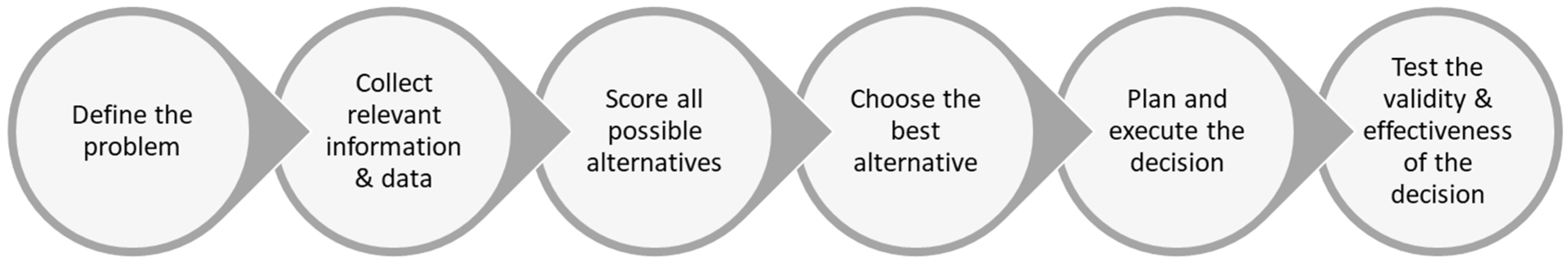
Effective decision making is a crucial aspect of management across all industries, as it is often considered the primary function of any management team. The decisions made can have a significant impact on an organization’s growth in various areas, and each decision-making process aims to achieve specific goals that enable the organization to expand and succeed in multiple directions. However, organizations encounter several obstacles in fulfilling their objectives, particularly in areas such as administration, marketing, operations, and finance. As a result, decision-making processes are employed to effectively overcome these challenges and accomplish their goals [40]. To achieve this, [41] argues that the process of making a decision can be divided into six distinct steps, as demonstrated in Figure 1.

Different decision-making methods can be categorized based on the techniques they employ, such as multiple-criteria decision-making (MCDM), mathematical programming (MP), artificial intelligence (AI), and theory-based methods [42]. MCDM, for instance, is a multi-step process that involves structuring and executing a formal decision-making process, assessing multiple alternatives against various criteria, and providing a recommendation based on the best-fit alternatives, which have been evaluated under multiple criteria [43]. MP methods, as described in [44], aim to optimize objectives while accounting for various constraints and boundaries that stakeholders must consider when making decisions. Examples of MP methods include goal programming, linear programming, and stochastic programming. AI, on the other hand, refers to a machine’s ability to learn from past experiences, adapt to new inputs, and perform tasks that are similar to those executed by humans, as defined in [45]. AI systems can either assist or replace human decision makers.

As such, MCDM can handle conflicting quantitative and qualitative criteria, enabling decision makers to select the best-fit alternatives from a set of options in uncertain and risky situations [46]. This study therefore considers the MCDM to be the most suitable model making strategic smart campus decisions. The main MCDM approaches will be presented in the next section.

2.7. Multi-Criteria Decision-Making Method

The process of Multicriteria Decision-Making (MCDM) is complex and dynamic, consisting of two levels: managerial and engineering. At the managerial level, objectives are identified, and the most advantageous option, deemed “optimal”, is selected. This level emphasizes the multicriteria aspect of decision-making, and the decision makers, usually public officials, have the power to accept or reject the proposed solution from the engineering level [47]. Belton and Stewart in [48] describe MCDM as an “umbrella term to describe a collection of formal approaches which seek to take explicit account of multiple criteria in helping individuals or groups of individuals to explore decisions that matter”. In other words, MCDM is a valuable approach when there are various criteria that have conflicting priorities and are valued differently by stakeholders and decision makers. It becomes easier to assess multiple courses of action based on these criteria, which are crucial aspects of the decision-making process that involve human judgement and preferences. As a result of this evident benefit, MCDM has become increasingly popular and widely used in recent decades.

Furthermore, there is a vast range of MCDM techniques in the literature, each with its own strengths and weaknesses. One popular approach is the outranking synthesis method, which connects alternatives based on the decision maker’s preferences and helps to identify the best solution. PROMETHEE and ELECTRE are two examples of this method [49]. Another technique is the interactive local judgement (ILJ) approach, which involves a cycle of computation and discussion to produce successive solutions and gather additional information about the decision maker’s preferences [50,51]. Other approaches include Multi-Attribute Utility Theory (MAUT), simple multi-attribute rating technique (SMART), and analytic hierarchy process (AHP). Each of these methods offers unique advantages and disadvantages, and the choice of which one to use depends on the specific context of the decision-making problem. The following paragraph explores the strengths and weaknesses of each of the main MCDM methods [18,49,52,53,54,55]:

–

ELECTRE: iterative outranking method based on concordance analysis that can consider uncertainty and vagueness. However, it is not easily explainable, and the strengths and weaknesses of the alternatives are not clearly identified.

–

PROMETHEE: An outranking method that has several versions for partial ranking, complete ranking, and interval-based ranking. It is easy to use, but it does not provide a clear method to assign weights to the different criteria.

–

Analytic hierarchy process (AHP): A decision-making technique that makes pairwise comparisons among various options and factors. It is easy to apply and is scalable, but there is a risk of rank reversal and inconsistencies between judgment and ranking criteria.

–

Technique for order of preference by similarity to an ideal solution (TOPSIS): A method that identifies two alternatives based on their distance to an ideal solution in a multidimensional computing space. It is easy to use and has a simple process, but it relies on Euclidean distance to obtain the solution, which ignores the correlation of the attributes.

–

Multi-Attribute Utility Theory (MAUT): A method that assigns a level of usefulness or value to every potential result and then identifies the option with the greatest utility. It can take uncertainty into account and incorporate the preferences of the decision maker, but it is data-intensive.

–

Fuzzy set theory: useful for dealing with imprecise and uncertain data but difficult to develop and requiring multiple simulations before use.

–

Case-based Reasoning (CBR): Retrieves cases similar to the current decision-making problem from an existing database of cases and proposes a solution based on previous solutions. It is not data-intensive and requires little maintenance, but is sensitive to inconsistent data.

–

Data envelopment analysis (DEA): Measures the relative efficiencies of alternatives against each other and can handle multiple inputs and outputs. It cannot deal with imprecise data.

–

Simple multi-attribute rating technique (SMART): One of the most basic types of MAUT that is simple and requires less effort by decision-makers. However, it may not be convenient for complex real-life decision-making problems, where criteria affecting the decision-making process are usually interrelated.

–

Goal programming: can solve a decision-making problem from infinite alternatives but needs to be used in combination with other MCDM methods to determine the weight coefficients.

–

Simple additive weighting (SAW): Establishes a value function based on a simple addition of scores representing the goal achievement under each criterion, multiplied by particular weights. It is easy to understand and apply, but it may not be suitable for complex decision-making problems.

–

Evidential reasoning (ER): The evidential reasoning (ER) approach is a decision support framework that uses a belief structure to address decision-making problems involving qualitative and quantitative criteria. ER combines the utility theory, probability theory, and theory of evidence to define decision problems and aggregate evidence. The approach comprises two components: the knowledge base and the inference engine. The knowledge base includes domain knowledge, decision parameters, additional factors, and user beliefs. The inference engine uses the Dempster–Shafer theorem to define probability and evaluation grades and combine beliefs. ER handles both qualitative and quantitative attributes, avoids distortion of data during transformation, and handles stochastic and incomplete attributes. ER provides accurate and precise data while capturing various types of uncertainties.

When it comes to developing decision-making tools for optimizing smart campus applications, ER stands out as the best approach due to its unique ability to handle both qualitative and quantitative attributes without introducing any data distortion. Furthermore, ER is highly effective at handling uncertain and incomplete attributes in a stochastic environment, making it an ideal method for strategic decision-making. With its superior accuracy and precision, ER can capture various types of uncertainties that may arise.

The next section, therefore, delves into the theory underlying the approach in greater detail, elucidating its mathematical formulation, including parameters such as aggregated probability mass, degrees of belief, and utility. By presenting a more in-depth analysis of these key concepts, this section will provide a comprehensive understanding of the approach and its underlying principles, which will be used by this study to develop the decision support tool for a smart campus.

2.8. Evidential Reasoning Approach

The ER approach combines input information and infers evidence for an alternative using the Dempster–Shafer (DS) hypothesis [56]. The approach deals with a multi-criteria decision problem with L basic attributes under a general attribute Y. Since the utility of the general attribute Y is challenging to measure directly, several more operational indicators are measured to estimate it, which are the basic attributes. Thus, a general attribute can be divided into basic attributes. Table 2 presents the main parameters used in the ER approach.

Table 2. Main parameters used in the ER approach [56,57].

Parameter	Description
Basic Attributes, A	$A=\left\{a_1,a_2,\dots ,a_i,\dots ,a_L\right\},$ L: Number of basic Attributes
Evaluation Grades of an alternative, E	$E={\{e}_1,e_2,\dots ,e_n,\dots ,e_N\}$ N: Number of Evaluation Grades
User Beliefs (degrees of belief), ${\beta }_{i,n}$	$$0\le {\sum }_{n=1}^N{\beta }_{i,n}\le 1\forall i$$ (1) ${\beta }_{i,n}$ denoting the degree of belief for the basic attribute ai at the evaluation grade en (Degree to which the user is confident about a particular assertion). A complete assessment of an attribute means ${\sum }_{n=1}^N{\beta }_{i,n}=1$ An incomplete assessment of an attribute means ${\sum }_{n=1}^N{\beta }_{i,n}<1$
Attribute Weights, ${\omega }_i$	$$0\le {\omega }_i\le 1\forall i$$ (2) $${\sum }_{i=1}^L{\omega }_i=1$$ (3) Each attribute needs to be assigned a weight.
Utilities, $u_n$	Determine the desirability of an alternative where a highest possible utility value of 1 should be assigned to the most desirable evaluation grade en.
	The probability mass of a basic attribute ai at evaluation grade en. It represents how well $a_i$ supports the claim that the assessment of y is $e_n$. $$m_{i,n}={\omega }_i·{\beta }_{i,n}$$ (4) In case of uncertainty, $$m_i^{*}=1-{\sum }_{n=1}^N{m}_{i,n}=1-{\omega }_i{\sum }_{n=1}^N{\beta }_{i,n}$$ (5) $m_i^{*}$ can be decomposed into two components: ${\underline{m}}_i$ and ${\tilde{m}}_i$. ${\underline{m}}_i$ is the remaining probability mass unassigned to attribute $a_i$ due to incomplete weight, while ${\tilde{m}}_i$ is the remaining probability mass unassigned to attribute $a_i$ due to incomplete degree of belief. $${\underline{m}}_i=1-{\omega }_i$$ (6) $${\tilde{m}}_i={\omega }_i\left(1-{\sum }_{n=1}^N{\beta }_{i,n}\right)$$ (7)

Table 2. Main parameters used in the ER approach [56,57].

Parameter	Description
Basic Attributes, A	$A=\left\{a_1,a_2,\dots ,a_i,\dots ,a_L\right\},$ L: Number of basic Attributes
Evaluation Grades of an alternative, E	$E={\{e}_1,e_2,\dots ,e_n,\dots ,e_N\}$ N: Number of Evaluation Grades
User Beliefs (degrees of belief), ${\beta }_{i,n}$	$$0\le {\sum }_{n=1}^N{\beta }_{i,n}\le 1\forall i$$ (1) ${\beta }_{i,n}$ denoting the degree of belief for the basic attribute ai at the evaluation grade en (Degree to which the user is confident about a particular assertion). A complete assessment of an attribute means ${\sum }_{n=1}^N{\beta }_{i,n}=1$ An incomplete assessment of an attribute means ${\sum }_{n=1}^N{\beta }_{i,n}<1$
Attribute Weights, ${\omega }_i$	$$0\le {\omega }_i\le 1\forall i$$ (2) $${\sum }_{i=1}^L{\omega }_i=1$$ (3) Each attribute needs to be assigned a weight.
Utilities, $u_n$	Determine the desirability of an alternative where a highest possible utility value of 1 should be assigned to the most desirable evaluation grade en.
	The probability mass of a basic attribute ai at evaluation grade en. It represents how well $a_i$ supports the claim that the assessment of y is $e_n$. $$m_{i,n}={\omega }_i·{\beta }_{i,n}$$ (4) In case of uncertainty, $$m_i^{*}=1-{\sum }_{n=1}^N{m}_{i,n}=1-{\omega }_i{\sum }_{n=1}^N{\beta }_{i,n}$$ (5) $m_i^{*}$ can be decomposed into two components: ${\underline{m}}_i$ and ${\tilde{m}}_i$. ${\underline{m}}_i$ is the remaining probability mass unassigned to attribute $a_i$ due to incomplete weight, while ${\tilde{m}}_i$ is the remaining probability mass unassigned to attribute $a_i$ due to incomplete degree of belief. $${\underline{m}}_i=1-{\omega }_i$$ (6) $${\tilde{m}}_i={\omega }_i\left(1-{\sum }_{n=1}^N{\beta }_{i,n}\right)$$ (7)

To evaluate an alternative’s overall performance on the general attribute y in the evidential reasoning approach, it is necessary to aggregate the data at the basic attribute level. This aggregation is carried out through a recursive algorithm, which performs L-1 iterations. At each recursion, the algorithm computes several measures that are aggregated across the basic attributes $a_1$ to $a_j$, where $j=\left\{2,\dots ,L\right\}$:

• $M_{j,n}$ denotes the probability mass aggregated at evaluation grade $e_n$. It is calculated as:

  $$M_{j,n}=K_j\left[M_{j-1,n}·m_{j,n}+M_{j-1}^{*}·m_{j,n}+M_{j-1,n}·m_j^{*}\right]$$

  (8)
• $K_j$ is a normalization factor that ensures the aggregated probability masses remain between 0 and 1 in each recursion of the ER algorithm. It is calculated as:

  $$K_j={[1-{\sum }_{t=1}^N{\sum }_{k=1k\ne t}^N{M}_{j-1,t}·m_{j,k}]}^{-1}\forall j=\left\{2,\dots ,L\right\}$$

  (9)
• $M_j^{*}$ is the unassigned probability mass aggregated over all evaluation grades. It is the sum of ${\underline{M}}_j$ and ${\tilde{M}}_j$.

  $$M_j^{*}={\underline{M}}_j+{\tilde{M}}_j$$

  (10)
• ${\underline{M}}_j$ is the unassigned probability mass due to incomplete weight, aggregated over all evaluation grades. It is calculated as:

  $${\underline{M}}_j=K_j\left[{\underline{M}}_{j-1}·{\underline{m}}_j\right]\forall j=\left\{2,\dots ,L\right\}$$

  (11)
• ${\tilde{M}}_j$ is the unassigned probability mass due to due to incomplete degrees of belief, aggregated across the basic attributes $a_1$ to $a_j$ and all evaluation grades. It is calculated as:

  $${\tilde{M}}_j=K_j\left[{\tilde{M}}_{j-1}·{\tilde{m}}_j+{\underline{M}}_{j-1}·{\tilde{m}}_j+{\tilde{M}}_{j-1}·{\underline{m}}_j\right]\forall j=\left\{2,\dots ,L\right\}$$

  (12)

  where:

  $$M_{1,n}=m_{1,n},{\underline{M}}_1={\underline{m}}_1,{\tilde{M}}_1={\tilde{m}}_1$$

  (13)

Once the aggregated probability masses $M_{L,n}$, ${\underline{M}}_L$, and ${\tilde{M}}_L$ have been calculated through the recursive ER algorithm, the aggregated degrees of belief can be calculated, where $B_n$ is the aggregated degree of belief for the general attribute y assessed to the evaluation grade $e_n$:

$$B_n=\frac{M_{L,n}}{1-{\underline{M}}_L}\forall n$$

(14)

whereas the unassigned, aggregated degree of belief for the general attribute y is $B^{*}$:

$$B^{*}=1-{\sum }_{n=1}^N{B}_n=\frac{{\tilde{M}}_L}{1-{\underline{M}}_L}$$

(15)

Finally, the aggregated utility for y is denoted by $U$. Under a complete assessment with no assessment uncertainty, the aggregated utility is calculated:

$$U={\sum }_{n=1}^N{B}_n{u}_n$$

(16)

However, if assessment uncertainty exists, i.e., there exists an unassigned belief, then a utility interval $[U_{min},U_{max}]$ is calculated instead, where $U_{min}$ and $U_{max}$ are the minimum and maximum utilities of y for the considered alternative, respectively. The endpoints of the utility interval are defined in the equations below.

$$U_{min}={\sum }_{n=1}^N{B}_n{u}_n+B^{*}{u}_N$$

(17)

$$U_{max}={\sum }_{n=1}^N{B}_n{u}_n+B^{*}{u}_1$$

(18)

Thus, the average aggregated utility, $U_{avg}$, is the midpoint of the utility interval:

$$U_{avg}=\frac{U_{max}+U_{min}}{2}$$

(19)

The model evaluates different alternatives by assigning utility values to each alternative based on various criteria. These utility values are then used to calculate an average aggregated utility value for each alternative, which is used to determine the optimal alternative.

The ER approach serves as the backbone of our decision support tool. It involves multiple stages:

Attribute weight determination: A panel of experts was engaged, comprising faculty, staff, and operational managers, to establish the relative importance of attributes. Utilizing the Nominal Group Technique, experts provided their final voted weights, which were then used as input for the ER model.

Model implementation and programming: The ER model, driven by the established attribute weights, was programmed in Python. This model processes belief tensors, which are three-dimensional matrices representing degrees of belief at the intersection of alternative, attribute, and evaluation grade. Python coding ensured efficient computation of average utility for each alternative and its subsequent ranking.

Validation and reliability: The model’s validity was rigorously tested. A paired t-test was utilized to compare the model-generated results with expert-provided results, while the Receiver Operating Characteristics (ROC) curve analysis was conducted to evaluate the model’s performance. Key metrics including accuracy, precision, sensitivity, specificity, negative predicted value, and F1 score, which were utilized for a comprehensive evaluation.

3. Data Collection, Implementation, Results and Validation

This section shares the data collection process and analysis conducted to develop the proposed evidential reasoning decision support tool for a smart campus. As such, two of the key components of the proposed decision tool are validated; namely, alternatives and attribute weights, using two different surveys. Attribute weights are then tested through weight perturbations. To ensure the model’s accuracy and reliability, various statistical tests are employed. All of the relevant ethical approval considerations for data collection have been followed, and the Institutional Research Board consent was granted prior to the data collection process.

3.1. Validation of Smart Campus Alternative Applications

To validate nine functional families of smart campus applications detailed in Section 2.4, a survey was conducted targeting 56 stakeholders from a renowned higher education institution, including students, alumni, and staff who were not necessarily smart campus experts. The participants were asked to rate the importance of the smart campus applications on a scale from 0 to 5. The results of the average scores and analysis of variance data are shown in

Table 3. Data summary for the stakeholders’ opinion survey.

Groups	Count	Sum	Average	Variance
A.1. Smart Learning Management System	56	242	4.321428571	0.512987013
A.2. Smart Campus Operations	56	252	4.5	0.290909091
A.3. Safe Learning Environment	56	230	4.107142857	1.188311688
A.4. Smart Geographic Information System	56	219	3.910714286	1.100974026
A.5. Smart Administrative System	56	245	4.375	0.565909091
A.6. Waste and Water Management System	56	243	4.339285714	0.700974026
A.7. Sustainable Energy Management System	56	244	4.357142857	0.815584416
A.8. Smart Classrooms	56	215	3.839285714	0.937337662
A.9. Smart Transportation System	56	235	4.196428571	0.778896104

below.

In addition, the stakeholders’ opinion data were subjected to a single-factor, two-way ANOVA test to determine if the proposed smart campus alternatives represented distinct categories. The ANOVA test results presented in

Table 4. Results of the single-factor, two-way ANOVA test on stakeholder survey data.

ANOVA
Source of Variation	SS	df	MS	F	p-Value	F Crit
Between Groups	22.37	8.00	2.7966	3.6521	0.0004	1.9571
Within Groups	379.05	495.00	0.7658
Total	401.43	503.00

show a statistically significant difference in stakeholder preference among the nine alternatives, with a p-value of 0.0004.

In conclusion, the survey conducted among 56 stakeholders demonstrated positive ratings for all nine functional families of smart campus applications. The stakeholders’ opinions exhibited significant variation among the different alternatives, as supported by the statistically significant results of the single-factor, two-way ANOVA test (p-value = 0.0004). This analysis confirmed that the proposed smart campus alternatives represent distinct categories, each with its own level of stakeholder preference. The obtained findings not only validate the selection of the nine smart campus applications but also provide valuable insights for the implementation of the ER decision tool. With the endorsement of these alternatives by the stakeholders, the ER decision tool can now be developed using these nine categories as input.

3.2. Attribute Weights

The evidential reasoning (ER) approach is a decision-making framework that combines input information to infer evidence for a particular alternative using the Dempster–Shafer (DS) hypothesis [57]. It is particularly useful for addressing multi-criteria decision problems that involve L basic attributes under a general attribute y. Directly measuring the utility of the general attribute can be difficult, so the approach relies on several more operational indicators, which are the basic attributes, to estimate it. This allows the general attribute to be divided into more manageable basic attributes. To depict the relationship between the general and basic attributes, an Architectural Theory Diagram (ATD) is used, which consists of a two-layer hierarchy (as shown in Figure 2). In this study, the basic attributes used in the decision support tool were derived from the critical success factors identified in the literature, including implementation cost, operation cost, maintenance cost, project duration, stakeholder benefits, and resource availability.

When faced with an MCDM problem, it is common to assign weights to decision attributes based on their relative importance. However, since historical data to derive weights for decision attributes may not always be available, a weight allocation logic must be employed [58]. In this study, a consensus-based approach was used to collect weights for the decision-making framework. Two popular consensus methods are the Delphi and the Nominal Group Technique (NGT) [59]. For this research, the NGT method [60,61] was proposed to allocate weights to decision attributes. Nine domain experts (Group A experts) assigned weights to decision parameters, discussed and justified their assigned weights for each attribute, and revised them if necessary. The facilitator then determined the final weight of each attribute through a voting process. The attribute weights collected through the NGT are summarized in

Table 5. Attribute weights provided by Group A experts.

General Attributes	Exp. 1	Exp. 2	Exp. 3	Exp. 4	Exp. 5	Exp. 6	Exp. 7	Exp. 8	Exp. 9	Average Weights
Implementation Cost	0.2	0.2	0.25	0.3	0.2	0.2	0.3	0.3	0.25	0.20
Maintenance Cost	0.15	0.10	0.2	0.1	0.10	0.15	0.1	0.1	0.1	0.10
Operation Cost	0.15	0.15	0.15	0.1	0.15	015	0.1	0.1	0.2	0.15
Project Duration	0.15	0.15	0.1	0.1	0.15	0.15	0.1	0.1	0.1	0.15
Stakeholder’s Benefit	0.2	0.25	0.2	0.3	0.25	0.2	0.3	0.3	0.25	0.25
Resource Availability	0.15	0.15	0.1	0.1	0.15	0.15	0.1	0.1	0.1	0.15

for easy reference, with the final weights obtained by averaging the attribute weights.

The attributes considered in the ER approach include implementation cost, maintenance cost, operation cost, project duration, stakeholder benefits, and resource availability. The attribute weights collected through the consensus-based approach using the NGT are crucial for the decision-making tool. These weights represent the relative importance of each attribute in the ER approach and play a vital role in evaluating smart campus alternative applications. By assigning weights to these attributes, the decision tool can effectively prioritize and assess the smart campus alternative applications based on their performance in these key areas.

3.3. Decision-Making Scenarios Generation

To validate the decision tool, belief tensors were randomly generated and given to five decision-making experts (referred to as Group B) who had more than 7 years of experience in decision-making tasks. Each expert was provided with 10 decision-making scenarios represented by 10 belief tensors. Each tensor was three-dimensional, consisting of 162 degrees of belief, since each run of the model requires a degree of belief to be reported at the intersection of the six attributes in Table 5, the nine smart campus alternative categories in Section 2.4, and the Figure 2 evaluation grades of the attributes listed in

Table 6. Evaluation grades for each attribute.

General Attributes	Evaluation Grades
Development Cost	Low (Good), Medium (Average), High (Poor)
Maintenance Cost	Low (Good), Medium (Average), High (Poor)
Operation Cost	Low (Good), Medium (Average), High (Poor)
Implementation Duration	Short (Good), Medium (Average), Long (Poor)
Stakeholder’s Benefit	High (Good), Medium (Average), Low (Poor)
Resource Availability	Yes (Good), Not Sure (Average), No (Poor)

, below.

A belief tensor was presented using a spreadsheet file (see

Table 7. Example of a generated decision-making scenario.

Attribute	Evaluation Grade	Alternatives
		A1	A2	A3	A4	A5	A6	A7	A8	A9
Implementation Cost	Good	0	0.5	0	0.3	0.9	0.7	0.1	0.6	0.4
	Average	0.5	0.5	0.5	0.3	0.05	0.3	0.2	0.3	0.6
	Poor	0.5	0	0.5	0.4	0.05	0	0.7	0.1	0
Operation Cost	Good	0.6	0.6	0.6	0.1	0.6	0.4	0.3	0.9	0.7
	Average	0.3	0.3	0.3	0.2	0.3	0.6	0.3	0.05	0.3
	Poor	0.1	0.1	0.1	0.7	0.1	0	0.4	0.05	0
Maintenance Cost	Good	0.1	0.6	0.4	0.3	0.9	0.7	0	0.5	0
	Average	0.2	0.3	0.6	0.3	0.05	0.3	0.5	0.5	0.5
	Poor	0.7	0.1	0	0.4	0.05	0	0.5	0	0.5
Stakeholder’s Benefit	Good	0	0.5	0	0.1	0.6	0.4	0.6	0.6	0.6
	Average	0.5	0.5	0.5	0.2	0.3	0.6	0.3	0.3	0.3
	Poor	0.5	0	0.5	0.7	0.1	0	0.1	0.1	0.1
Implementation Duration	Good	0.6	0.6	0.6	0	0.5	0	0.1	0.6	0.4
	Average	0.3	0.3	0.3	0.5	0.5	0.5	0.2	0.3	0.6
	Poor	0.1	0.1	0.1	0.5	0	0.5	0.7	0.1	0
Resource Availability	Good	0.4	0.25	0.4	0.1	0.6	0.4	0	0.5	0
	Average	0.6	0.25	0.6	0.2	0.3	0.6	0.5	0.5	0.5
	Poor	0	0.5	0	0.7	0.1	0	0.5	0	0.5

), where the user provides a degree of belief for each of the six attributes and nine alternatives against three evaluation grades on a scale of 0 to 1, representing the confidence level from 0 to 100%. To avoid overwhelming the experts, all 1620 elements were randomly generated and provided to the participants and they were asked to convert the given beliefs to utilities using their judgment and experience. This resulted in 50 sets of inputs and expert-provided outputs.

Corresponding to each belief tensor, each expert was also asked to select the best alternative, typically the ones which were assigned the maximum utility. The utilities provided by the experts and the corresponding optimal alternatives chosen by the experts are reported in Appendix A,

Table A1. Expert-provided utilities per alternative.

No.	Utilities									Optimal Alternative
	A1	A2	A3	A4	A5	A6	A7	A8	A9
1	1	0	0	0	0	0	0	0	0	A1
2	0	1	0	0	0	0	0	0	0	A2
3	0	0	1	0	0	0	0	0	0	A3
4	0	0	0	1	0	0	0	0	0	A4
5	0	0	0	0	1	0	0	0	0	A5
6	0	0	0	0	0	1	0	0	0	A6
7	0	0	0	0	0	0	1	0	0	A7
8	0	0	0	0	0	0	0	1	0	A8
9	0	0	0	0	0	0	0	0	1	A9
10	1	0	0	0	0	0	0	0	0	A1
11	1	0	0	0	0	0	0	0	0	A1
12	0.25	0.25	0.75	0.25	0.25	0.25	0.25	0.25	0.25	A3
13	0.25	0.25	0.25	0.75	0.25	0.25	0.25	0.25	0.25	A4
14	0.25	0.25	0.25	0.25	0.75	0.25	0.25	0.25	0.25	A5
15	0.25	0.25	0.25	0.25	0.25	0.75	0.25	0.25	0.25	A6
16	0.25	0.25	0.25	0.25	0.25	0.25	0.75	0.25	0.25	A7
17	0.25	0.25	0.25	0.25	0.25	0.25	0.25	0.75	0.25	A8
18	0.25	0.25	0.25	0.25	0.25	0.25	0.25	0.25	0.75	A9
19	0.5	0.2	0.2	0.2	0.2	0.2	0.2	0.2	0.2	A1
20	0.2	0.5	0.2	0.2	0.2	0.2	0.2	0.2	0.2	A2
21	0.2	0.2	0.5	0.2	0.2	0.2	0.2	0.2	0.2	A3
22	0.2	0.2	0.2	0.5	0.2	0.2	0.2	0.2	0.2	A4
23	0.2	0.2	0.2	0.2	0.5	0.2	0.2	0.2	0.2	A5
24	0.2	0.2	0.2	0.2	0.2	0.5	0.2	0.2	0.2	A6
25	0.2	0.2	0.2	0.2	0.5	0.2	0.5	0.2	0.2	A7
26	0.2	0.2	0.2	0.2	0.5	0.2	0.2	0.5	0.2	A8
27	0.2	0.2	0.2	0.2	0.5	0.2	0.2	0.5	0.2	A8
28	0.5	0.5	0.6	0.6	0.6	0.7	0.6	0.65	0.5	A6
29	0.59	0.67	0.45	0.49	0.49	0.6	0.58	0.58	0.7	A9
30	0.65	0.7	0.45	0.55	0.6	0.65	0.56	0.7	0.6	A2
31	0.7	0.75	0.5	0.4	0.65	0.6	0.6	0.75	0.6	A2
32	0.4	0.55	0.6	0.6	0.6	0.75	0.6	0.65	0.7	A6
33	0.6	0.6	0.6	0.72	0.55	0.65	0.7	0.15	0.7	A4
34	0.651	0.65	0.6	0.6	0.6	0.7	0.6	0.7	0.15	A6
35	0.7	0.15	0.65	0.65	0.6	0.6	0.6	0.7	0.55	A1
36	0.15	0.65	0.65	0.6	0.7	0.55	0.6	0.6	0.7	A5
37	0.15	0.65	0.7	0.6	0.7	0.55	0.6	0.6	0.7	A9
38	0.6	0.7	0.55	0.7	0.65	0.65	0.15	0.65	0.6	A2
39	0.45	0.7	0.5	0.25	0.8	0.7	0.35	0.8	0.6	A5
40	0.45	0.75	0.55	0.65	0.55	0.8	0.65	0.55	0.55	A6
41	0.75	0.5	0.8	0.7	0.6	0.78	0.75	0.5	0.7	A3
42	0.6	0.3	0.6	0.6	0.5	0.6	0.3	0.75	0.4	A8
43	0.65	0.55	0.8	0.7	0.5	0.7	0.45	0.6	0.7	A3
44	0.3	0.6	0.7	0.5	0.8	0.65	0.3	0.5	0.65	A5
45	0.3	0.45	0.55	0.3	0.6	0.5	0.2	0.8	0.45	A8
46	0.65	0.65	0.8	0.7	0.55	0.85	0.55	0.55	0.7	A6
47	0.6	0.15	0.45	0.4	0.3	0.45	0.3	0.6	0.45	A8
48	0.5	0.45	0.5	0.4	0.4	0.7	0.5	0.65	0.35	A6
49	0.4	0.35	0.45	0.4	0.45	0.45	0.4	0.55	0.35	A8
50	0.65	0.4	0.6	0.35	0.5	0.45	0.35	0.45	0.45	A1

.

In order to validate the performance of the developed decision-making support tool, the utilities and optimal choices determined by the decision-making experts for the 50 randomly generated scenarios (

Table 8. Case processing summary for t-test.

	Cases
	Valid		Missing		Total
	N	Percent	N	Percent	N	Percent
Decision-tool-Generated Utilities	50	100.0%	0	0.0%	50	100.0%
Expert-Provided Utilities	50	100.0%	0	0.0%	50	100.0%

) will be compared to those obtained by the decision tool. This comparison will be conducted in Section 3.7. By comparing the results from the decision-making experts with the outcomes produced by the decision tool, the validation process aims to assess the tool’s effectiveness and accuracy in determining utilities and optimal choices across various scenarios. This analysis will provide valuable insights into the tool’s performance, highlighting its strengths and areas for improvement. Through this validation process, stakeholders can gain confidence in the reliability of the decision-making support tool and its ability to assist in making informed choices.

3.4. Decision Support System Implementation

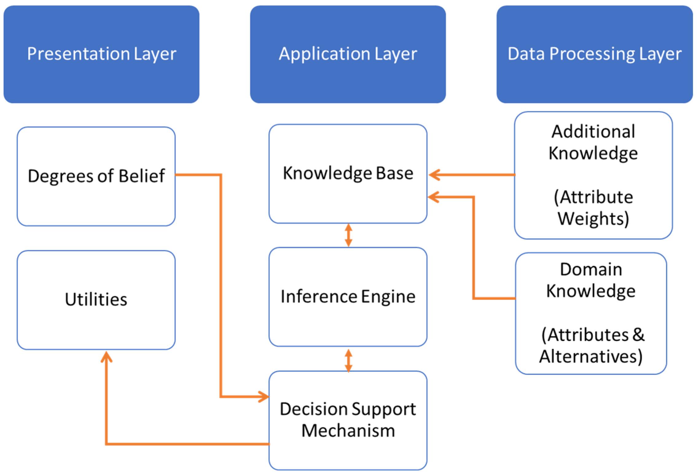
To implement the decision support tool effectively, two main components need to be developed: the knowledge capture matrix and the knowledge manipulation algorithms. The knowledge capture matrix is constructed based on findings from the literature review (nine different smart application alternatives), while the six attribute weights are provided by domain experts (Section 3.2). The knowledge manipulation, or aggregation engine, is developed using the Dempster–Shafer (DS) algorithm. The decision support tool is built using Python version 3.9, with the PyCharm Community Edition 2022.3.2 serving as the Integrated Development Environment (IDE). 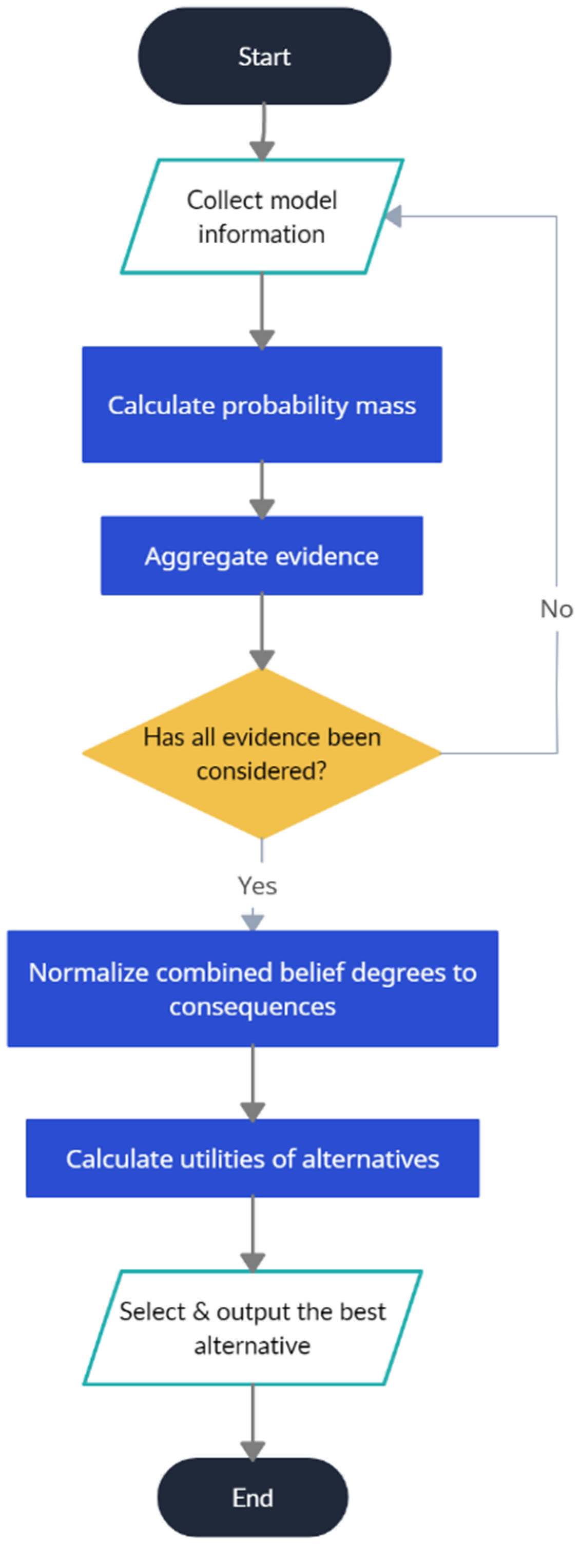The decision support‘s architecture is depicted in Figure 3, showcasing three structural layers [62]: the presentation, application, and data processing layers. The presentation layer acts as the user interface, allowing users to interact with the decision support tool. The application layer handles calculations and facilitates communication between different layers. The data processing layer contains the necessary knowledge resources. The decision support tool utilizes the inference engine based on the DS theory. This engine recursively combines probability masses and beliefs of basic attributes to generate utilities for decision alternatives. The evidential reasoning (ER) approach is used to normalize the combined probability masses.

The logic of the inference engine is illustrated in the flowchart presented in Figure 4.

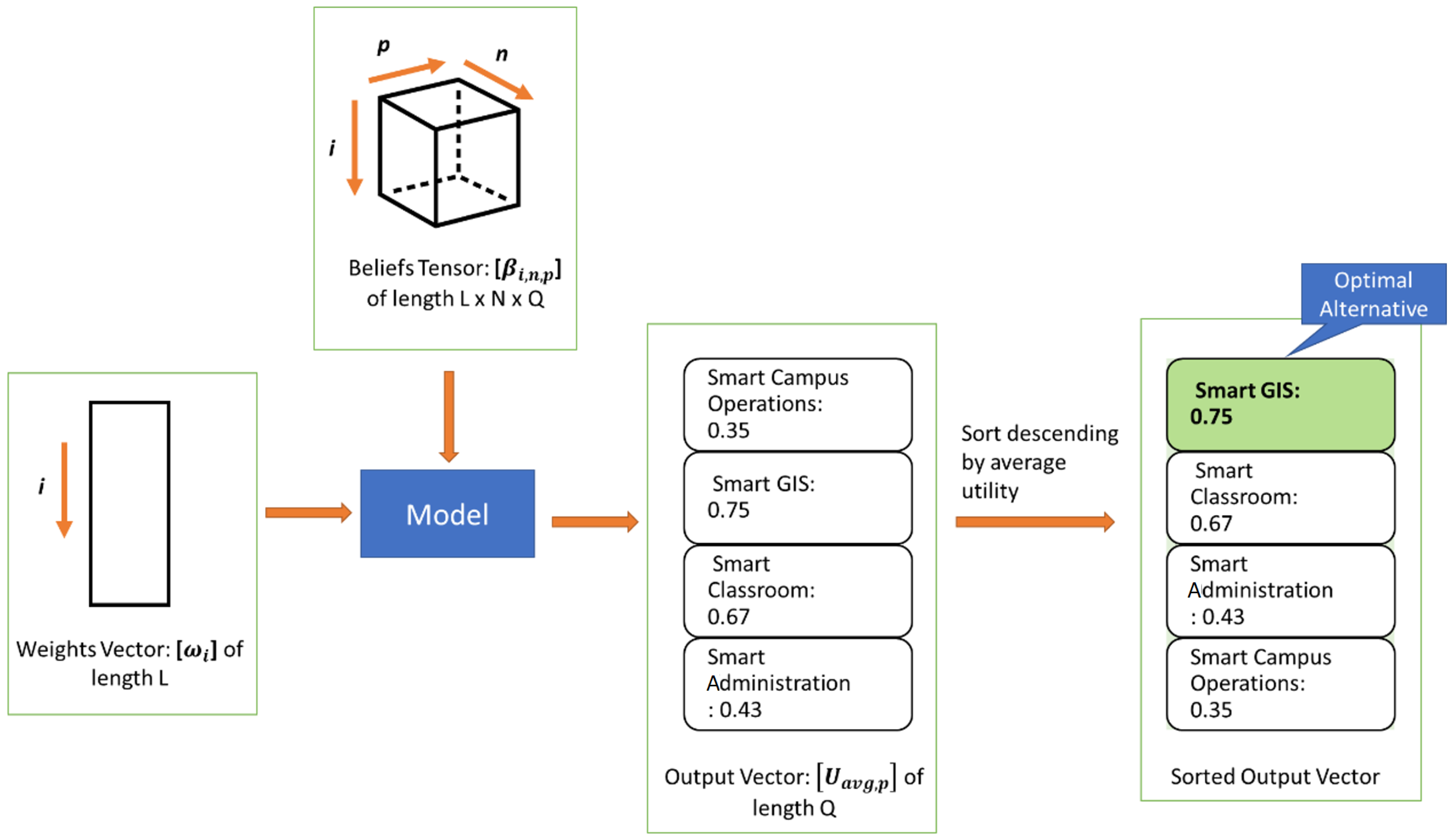
The decision tool relies on two essential inputs to function effectively: a vector of weight attributes, as developed in Section 3.2, and a beliefs tensor representing the user’s assessment of the nine smart campus alternative applications across the six attributes. By combining these inputs, the model is able to calculate the utility of each alternative, providing valuable insights for decision making. In the given example (Figure 5), the smart GIS (Geographical Information Systems) application for a smart campus emerges as the alternative with the highest utility value. It is closely followed by smart classroom applications, smart administration, and smart campus operations. These rankings are determined based on the calculated utility values, allowing stakeholders to identify the most favorable alternatives within the context of the assessed attributes.

The decision tool’s ability to generate utility values facilitates a comprehensive evaluation of the smart campus alternative applications, aiding stakeholders in making informed decisions regarding their implementation. By considering both the weighted attributes and the user’s assessment, the tool provides a structured approach for assessing and comparing the potential benefits of different alternatives, enabling the identification of the most suitable options for a smart campus environment.

The next section, the decision tool’s inputs and outputs are validated and its performance is assessed.

3.5. Validation of Attribute Weights

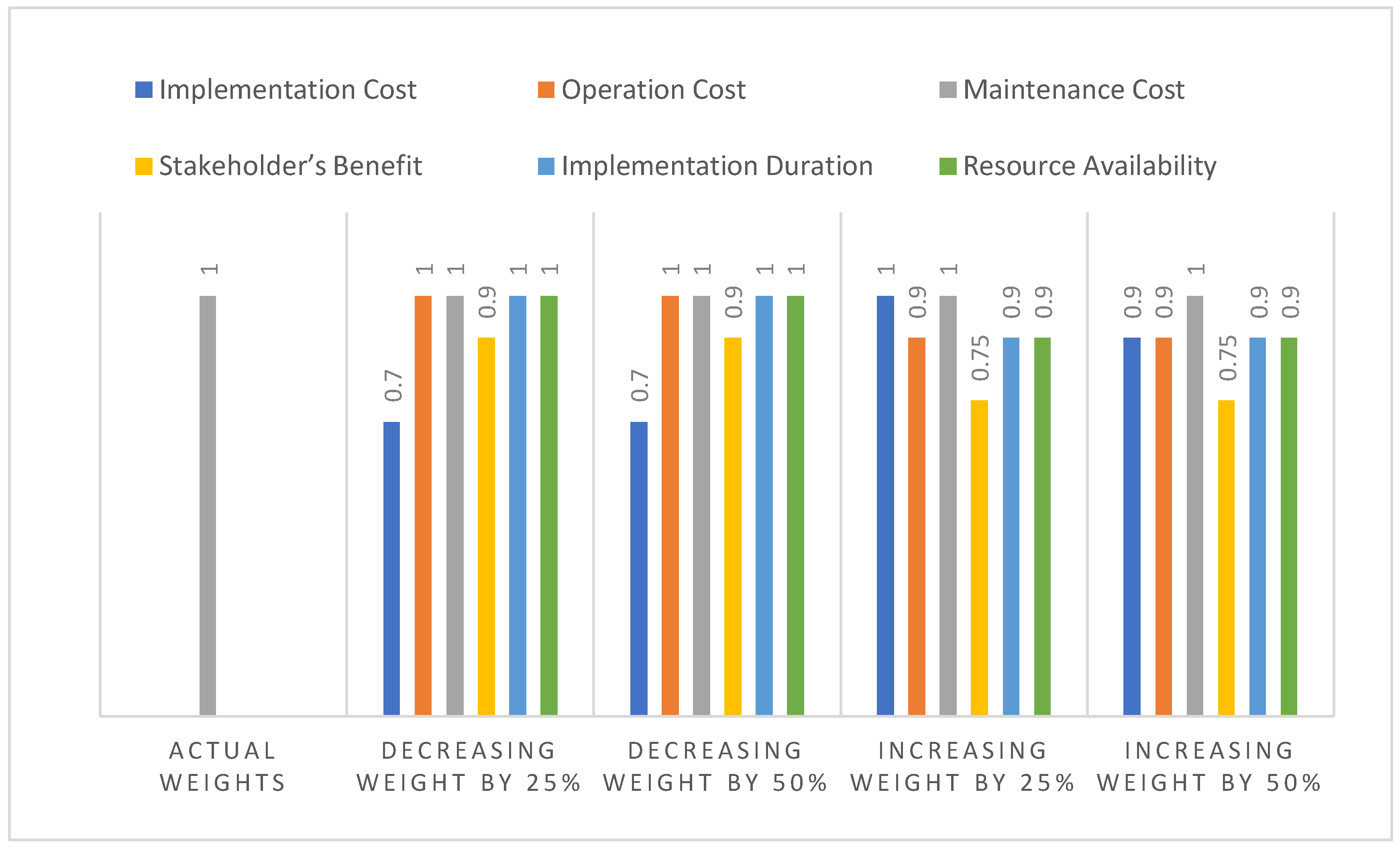
The attribute weights used in this study were collected through the NGT (Nominal Group Technique). To validate the attribute weights (determined in Section 3.2), the model’s sensitivity to weight perturbations was tested. Five belief tensors were chosen, which produced outputs identical to the expert-recommended alternatives. For each attribute, the weights were changed by 25% and 50%, resulting in four new sets of weights per attribute (as shown in Figure 6). The model was then run 24 times for each of the five belief tensors, resulting in a total of 120 runs. After each run, the optimal alternative and its utility were recorded and compared against expert-provided utilities. Additionally, the decision accuracy of the decision tool was compared to truth data, and confusion matrices were developed [62,63]. The decision tool performance was reported in terms of accuracy, sensitivity, and specificity for each set of weights.

Table A2. Attribute weight variation.

Attributes	Attribute Being Controlled	Actual Weight	Weight Decreased by 25%	Weight Decreased by 50%	Weight Increased by 25%	Weight Increased by 50%
		Set 1	Set 2	Set 3	Set 4	Set 5
Implementation Cost		0.2	0.15	0.1	0.25	0.3
Operation Cost		0.15	0.16	0.17	0.14	0.13
Maintenance Cost		0.1	0.11	0.12	0.09	0.08
Stakeholders’ Benefit		0.25	0.26	0.27	0.24	0.23
Implementation Duration		0.15	0.16	0.17	0.14	0.13
Resource Availability		0.15	0.16	0.17	0.14	0.13
Implementation Cost		0.2	0.2075	0.215	0.1925	0.185
Operation Cost		0.15	0.1125	0.075	0.1875	0.225
Maintenance Cost		0.1	0.1075	0.115	0.0925	0.085
Stakeholders’ Benefit		0.25	0.2575	0.265	0.2425	0.235
Implementation Duration		0.15	0.1575	0.165	0.1425	0.135
Resource Availability		0.15	0.1575	0.165	0.1425	0.135
Implementation Cost		0.2	0.205	0.21	0.195	0.19
Operation Cost		0.15	0.155	0.16	0.145	0.14
Maintenance Cost		0.1	0.075	0.05	0.125	0.15
Stakeholders’ Benefit		0.25	0.255	0.26	0.245	0.24
Implementation Duration		0.15	0.155	0.16	0.145	0.14
Resource Availability		0.15	0.155	0.16	0.145	0.14
Implementation Cost		0.2	0.2152	0.225	0.1875	0.175
Operation Cost		0.15	0.1625	0.175	0.1375	0.125
Maintenance Cost		0.1	0.1125	0.125	0.0875	0.075
Stakeholders’ Benefit		0.25	0.1875	0.125	0.3125	0.375
Implementation Duration		0.15	0.1625	0.175	0.1325	0.125
Resource Availability		0.15	0.1625	0.175	0.1375	0.125
Implementation Cost		0.2	0.2075	0.215	0.1925	0.185
Operation Cost		0.15	0.1125	0.075	0.1875	0.225
Maintenance Cost		0.1	0.1075	0.115	0.0925	0.085
Stakeholders’ Benefit		0.25	0.2575	0.265	0.2425	0.235
Implementation Duration		0.15	0.1575	0.165	0.1425	0.135
Resource Availability		0.15	0.1575	0.165	0.1425	0.135
Implementation Cost		0.2	0.2075	0.215	0.1925	0.185
Operation Cost		0.15	0.1125	0.075	0.1875	0.225
Maintenance Cost		0.1	0.1075	0.115	0.0925	0.085
Stakeholders’ Benefit		0.25	0.2575	0.265	0.2425	0.235
Implementation Duration		0.15	0.1575	0.165	0.1425	0.135
Resource Availability		0.15	0.1575	0.165	0.1425	0.135

of Appendix A summarizes how the attribute weights affect system performance, which can be more clearly visualized using the bar chart in Figure 6.

To compare the decision tool’s performance against expert-provided utilities, only the utilities of the optimal alternatives (shown in

Table A3. Variation in the utility of the optimal alternative due to change in weight.

0.55	Beliefs Tensor 5	0.66	Beliefs Tensor 4	0.61	Beliefs Tensor 3	0.85	Beliefs Tensor 2	0.81	Beliefs Tensor 1	Utilities under original weights
0.55		0.69		0.60		0.86		0.79		Implementation Cost	Decreasing Weight by 25%
0.54		0.68		0.64		0.86		0.81		Operation Cost
0.56		0.66		0.60		0.85		0.82		Maintenance Cost
0.59		0.65		0.65		0.84		0.79		Stakeholder’s Benefit
0.54		0.68		0.64		0.86		0.81		Implementation Duration
0.54		0.68		0.64		0.86		0.81		Resource Availability
0.55		0.74		0.59		0.87		0.77		Implementation Cost	Decreasing Weight by 50%
0.53		0.70		0.67		0.87		0.80		Operation Cost
0.66		0.66		0.60		0.85		0.58		Maintenance Cost
0.63		0.63		0.69		0.83		0.78		Stakeholder’s Benefit
0.53		0.70		0.67		0.87		0.80		Implementation Duration
0.53		0.70		0.67		0.87		0.80		Resource Availability
0.55		0.69		0.63		0.84		0.83		Implementation Cost	Increasing Weight by 25%
0.56		0.63		0.63		0.85		0.82		Operation Cost
0.54		0.66		0.62		0.85		0.80		Maintenance Cost
0.51		0.68		0.60		0.86		0.83		Stakeholder’s Benefit
0.56		0.63		0.63		0.85		0.82		Implementation Duration
0.56		0.63		0.63		0.85		0.82		Resource Availability
0.55		0.69		0.84		0.84		0.83		Implementation Cost	Increasing Weight by 50%
0.57		0.61		0.65		0.84		0.57		Operation Cost
0.52		0.67		0.63		0.85		0.79		Maintenance Cost
0.47		0.71		0.59		0.87		0.85		Stakeholder’s Benefit
0.57		0.61		0.65		0.84		0.57		Implementation Duration
0.57		0.61		0.65		0.84		0.57		Resource Availability

, Appendix A) were used. Furthermore, a comparison of the decision tool’s decision accuracy against the truth data was performed and reported in

Table A4. Variation in the optimal alternative due to changes in weight.

Actual Output	Decreasing Weight by 25%						Decreasing Weight by 50%						Increasing Weight by 25%						Increasing Weight by 50%
	Implementation Cost	Operation Cost	Maintenance Cost	Stakeholder’s Benefit	Implementation Duration	Resource Availability	Implementation Cost	Operation Cost	Maintenance Cost	Stakeholder’s Benefit	Implementation Duration	Resource Availability	Implementation Cost	Operation Cost	Maintenance Cost	Stakeholders Benefit	Implementation Duration	Resource Availability	Implementation Cost	Operation Cost	Maintenance Cost	Stakeholder’s Benefit	Implementation Duration	Resource Availability
Beliefs Tensor 1
A8	A8	A8	A8	A8	A8	A8	A8	A8	A8	A8	A8	A8	A8	A8	A8	A8	A8	A8	A8	A8	A8	A8	A8	A8
Beliefs Tensor 2
A6	A6	A6	A6	A6	A6	A6	A6	A6	A6	A6	A6	A6	A6	A6	A6	A6	A6	A6	A6	A6	A6	A6	A6	A6
Beliefs Tensor 3
A1	A8	A1	A1	A8	A1	A1	A8	A1	A1	A8	A1	A1	A1	A8	A1	A1	A8	A8	A6	A8	A1	A1	A8	A8
Beliefs Tensor 4
A8	A6	A8	A8	A8	A8	A8	A6	A8	A8	A8	A8	A8	A8	A8	A8	A6	A8	A8	A8	A8	A8	A6	A8	A8
Beliefs Tensor 5
A8	A8	A8	A8	A8	A8	A8	A8	A8	A8	A8	A8	A8	A8	A8	A8	A8	A8	A8	A8	A8	A8	A8	A8	A8

, Appendix A. Finally,

Table A5. Variation in the tool’s performance metrics due to change in weight.

Accuracy	Specificity	Sensitivity	Negative Predicted Value	Precision
1.0	1.0	1.0	1.0	1.0	Value under Original Weights
0.7	0.67	0.75	0.8	0.6	Implementation Cost	Decreasing Weight by 25%
1.0	1.0	1.0	1.0	1.0	Operation Cost
1.0	1.0	1.0	1.0	1.0	Maintenance Cost
0.9	0.83	1.0	1.0	0.8	Stakeholder’ s Benefit
1.0	1.0	1.0	1.0	1.0	Implementation Duration
1.0	1.0	1.0	1.0	1.0	Resource Availability
0.7	0.67	0.75	0.8	0.6	Implementation Cost	Decreasing Weight by 50%
1.0	1.0	1.0	1.0	1.0	Operation Cost
1.0	1.0	1.0	1.0	1.0	Maintenance Cost
0.9	0.83	1.0	1.0	0.8	Stakeholder’s Benefit
1.0	1.0	1.0	1.0	1.0	Implementation Duration
1.0	1.0	1.0	1.0	1.0	Resource Availability
1.0	1.0	1.0	1.0	1.0	Implementation Cost	Increasing Weight by 25%
0.9	0.83	1.0	1.0	0.8	Operation Cost
1.0	1.0	1.0	1.0	1.0	Maintenance Cost
0.75	0.75	0.75	0.75	0.75	Stakeholder’s Benefit
0.9	0.83	1.0	1.0	0.8	Implementation Duration
0.9	0.83	1.0	1.0	0.8	Resource Availability
0.9	0.83	1.0	1.0	0.8	Implementation Cost	Increasing Weight by 50%
0.9	0.83	1.0	1.0	0.8	Operation Cost
1.0	1.0	1.0	1.0	1.0	Maintenance Cost
0.75	0.75	0.75	0.75	0.75	Stakeholder’ s Benefit
0.9	0.83	1.0	1.0	0.8	Implementation Duration
0.9	0.83	1.0	1.0	0.8	Resource Availability

of Appendix A shows how the weights of attributes affect the decision tool’s performance. Figure 6 illustrates that the model’s accuracy varies with changes in attribute weights, thereby validating the weights collected through the ‘Nominal Group Technique.’

When expert-allocated weights are used, the model achieves 100% accuracy. Once the validated alternatives and weights were obtained, they were programmed into the tool, which was then run through 50 randomly generated belief tensors in the validation dataset. In the following section, various outputs for a single tool run are presented to demonstrate the decision tool’s performance.

3.6. Decision Tool Output

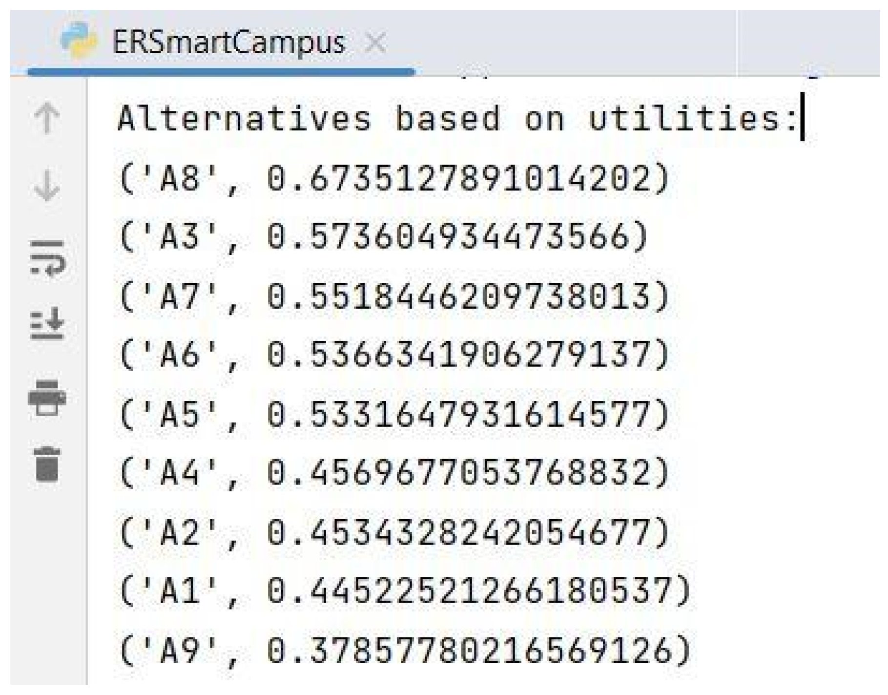
The main outputs of the proposed decision tool are a vector of the average utilities, denoted as $U_{avg}$, for each alternative. Additionally, the tool produces an optimally ranked list of the smart campus alternatives, in descending order of $U_{avg}$. If the end user wishes to receive a single recommendation, it can be obtained from the top alternative in the ranked list. The average utility of each alternative is demonstrated in the PyCharm console, as shown in Figure 7.

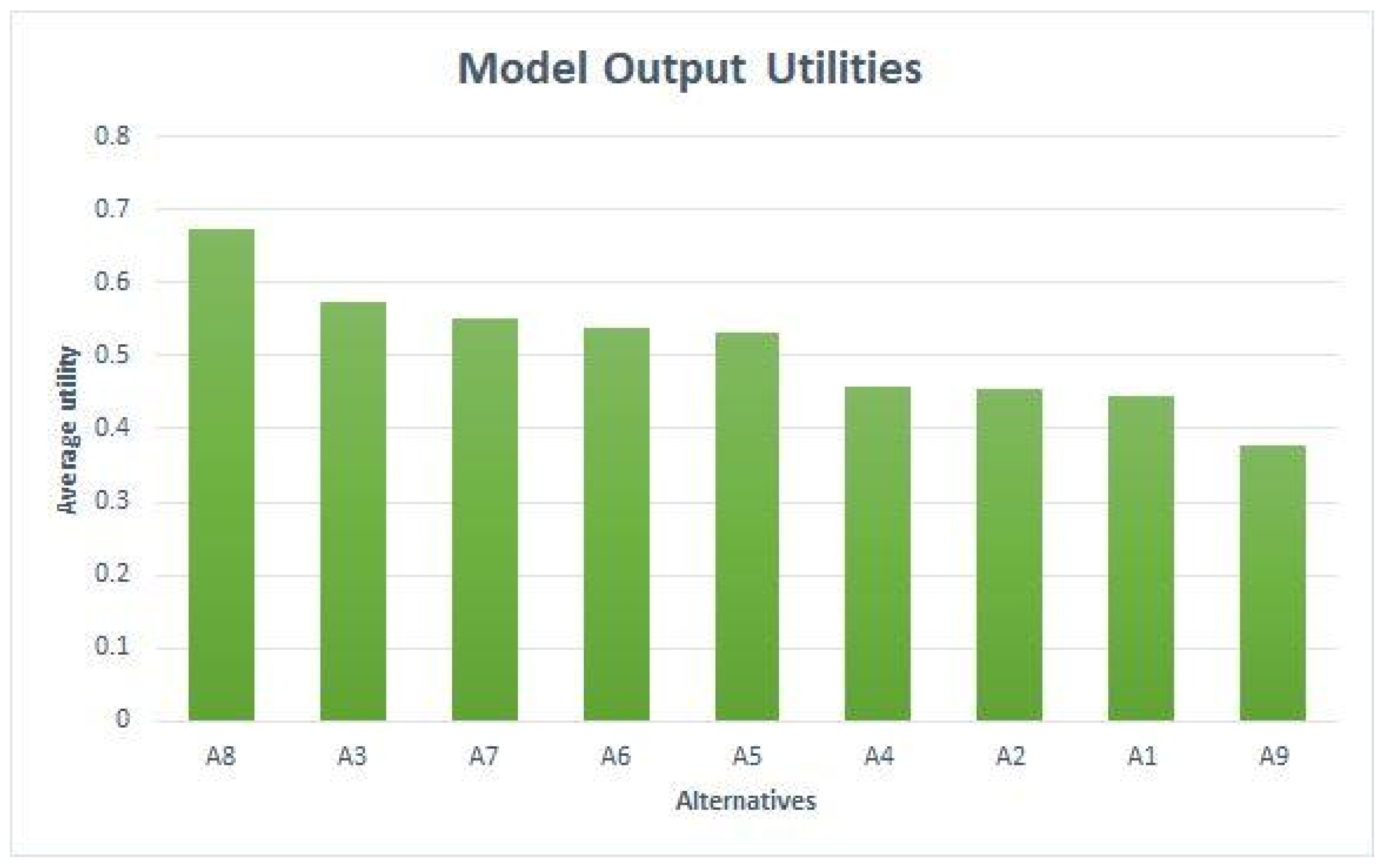
To make the results more accessible and understandable, the decision tool provides visual representations of the outputs using bar charts. Figure 8 presents a bar chart that displays the utilities of different smart campus alternatives. Among these alternatives, “A8” is recommended as the top choice for establishing the smart campus because it has the highest utility value. Additionally, the decision tool offers graphical reports of certain intermediary variables, which can be valuable for expert users who want to understand the results of the decision tool. 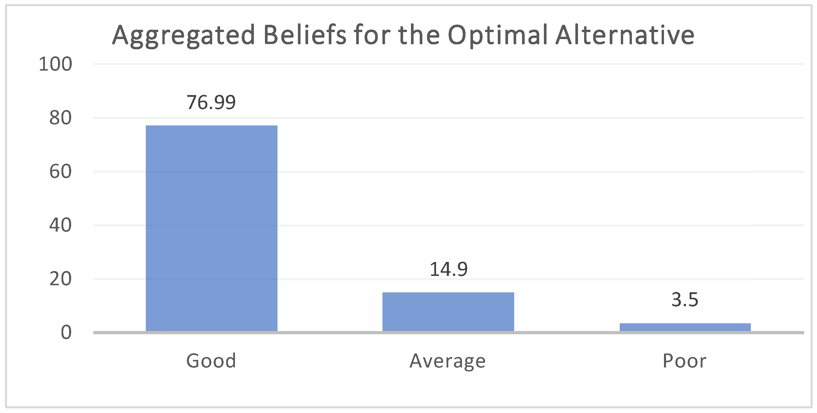One such variable is Bn, which represents the aggregated degree of belief by evaluation grade for an alternative.

Figure 9 illustrates a bar chart showing the Bn values for the optimal alternative. In this example, the optimal alternative received 77% of assessments as “good”, 14.9% as “average”, and only 3.5% as “poor”. This breakdown of assessments provides further insights into the decision-making process of the model, allowing users to better understand and interpret the outcomes. By presenting the results through visual representations, the decision tool enhances clarity and facilitates a more intuitive understanding of the outputs. These visualizations enable users to easily identify the recommended alternative and gain deeper insights into the underlying assessment and belief aggregation processes.

3.7. Decision Tool Validity

The decision tool was validated by comparing the utilities and optimal alternatives generated by the decision tool (

Table A6. Decision-tool-generated utilities based on the beliefs tensors provided to Group B.

Expert	Utilities Generated by Decision Tool									Output
	A1	A2	A3	A4	A5	A6	A7	A8	A9
1	1	0	0	0	0	0	0	0	0	A1
2	0	1	0	0	0	0	0	0	0	A2
3	0	0	1	0	0	0	0	0	0	A3
4	0	0	0	1	0	0	0	0	0	A4
5	0	0	0	0	1	0	0	0	0	A5
6	0	0	0	0	0	1	0	0	0	A6
7	0	0	0	0	0	0	1	0	0	A7
8	0	0	0	0	0	0	0	1	0	A8
9	0	0	0	0	0	0	0	0	1	A9
10	1	0	0	0	0	0	0	0	0	A1
11	1	0	0	0	0	0	0	0	0	A1
12	0.25	0.25	0.75	0.25	0.25	0.25	0.25	0.25	0.25	A3
13	0.25	0.25	0.25	0.75	0.25	0.25	0.25	0.25	0.25	A4
14	0.25	0.25	0.25	0.25	0.75	0.25	0.25	0.25	0.25	A5
15	0.25	0.25	0.25	0.25	0.25	0.75	0.25	0.25	0.25	A6
16	0.25	0.25	0.25	0.25	0.25	0.25	0.75	0.25	0.25	A7
17	0.25	0.25	0.25	0.25	0.25	0.25	0.25	0.75	0.25	A8
18	0.25	0.25	0.25	0.25	0.25	0.25	0.25	0.25	0.75	A9
19	0.5	0.1634	0.1634	0.1634	0.163	0.1634	0.1634	0.1634	0.1634	A1
20	0.1634	0.5	0.1634	0.1634	0.163	0.1634	0.1634	0.1634	0.1634	A2
21	0.1634	0.1634	0.5	0.1634	0.163	0.1634	0.1634	0.1634	0.1634	A3
22	0.1634	0.1634	0.1634	0.5	0.163	0.1634	0.1634	0.1634	0.1634	A4
23	0.1634	0.1634	0.1634	0.1634	0.5	0.1634	0.1634	0.1634	0.1634	A5
24	0.1634	0.1634	0.1634	0.1634	0.163	0.5	0.1634	0.1634	0.1634	A6
25	0.1634	0.1634	0.1634	0.1634	0.163	0.1634	0.5	0.1634	0.1634	A7
26	0.1634	0.1634	0.1634	0.1634	0.163	0.1634	0.1634	0.5	0.1634	A8
27	0.1634	0.1634	0.1634	0.1634	0.163	0.1634	0.1634	0.5	0.1634	A8
28	0.4270	0.5439	0.6079	0.6108	0.610	0.6946	0.5792	0.6784	0.4500	A6
29	0.5792	0.6784	0.4500	0.4270	0.543	0.6079	0.6108	0.6100	0.6946	A9
30	0.6784	0.6946	0.4270	0.5439	0.607	0.6108	0.6100	0.6946	0.5792	A2
31	0.7344	0.7419	0.5174	0.4291	0.642	0.6063	0.5967	0.7419	0.6082	A2
32	0.4270	0.5439	0.6079	0.6108	0.610	0.6946	0.5792	0.6629	0.6794	A6
33	0.6079	0.6108	0.6100	0.6946	0.579	0.6629	0.6794	0.1634	0.6946	A4
34	0.6629	0.6794	0.6079	0.6108	0.610	0.6946	0.5792	0.6946	0.1634	A6

) to the utilities and smart campus optimal alternatives collected from experts in Table 6, using 50 randomly generated belief tensors. Furthermore, for each belief tensor, the assigned expert was asked to select the best alternative with the highest utility.

3.7.1. Raw Data Summary

The decision tool was validated using a dataset of 50 truth data points. The decision-tool-generated utilities and optimal alternatives were compared to their expert-provided counterparts in

Table A7. Comparison of the decision tool’s results to the experts’ decisions.

Test Runs	Decision Tool Utility	Decision Tool Results	Expert Utility	Expert Results
1	1	A1	1	A1
2	1	A2	1	A2
3	1	A3	1	A3
4	1	A4	1	A4
5	1	A5	1	A5
6	1	A6	1	A6
7	1	A7	1	A7
8	1	A8	1	A8
9	1	A9	1	A9
10	1	A1	1	A1
11	1	A1	1	A1
12	0.75	A3	0.75	A3
13	0.75	A4	0.75	A4
14	0.75	A5	0.75	A5
15	0.75	A6	0.75	A6
16	0.75	A7	0.75	A7
17	0.75	A8	0.75	A8
18	0.75	A9	0.75	A9
19	0.5	A1	0.5	A1
20	0.5	A2	0.5	A2
21	0.5	A3	0.5	A3
22	0.5	A4	0.5	A4
23	0.5	A5	0.5	A5
24	0.5	A6	0.5	A6
25	0.5	A7	0.5	A7
26	0.5	A8	0.5	A8
27	0.5	A8	0.5	A8
28	0.69	A6	0.7	A6
29	0.69	A9	0.6	A9
30	0.694614	A2	0.7	A2
31	0.741931	A2	0.75	A2
32	0.694614	A6	0.75	A6
33	0.694614	A4	0.7	A4
34	0.694614	A6	0.7	A6
35	0.694614	A1	0.7	A1
36	0.694614	A5	0.7	A5
37	0.694614	A5	0.7	A9
38	0.694614	A2	0.7	A2
39	0.83354	A5	0.8	A5
40	0.797288	A6	0.8	A6
41	0.802289	A3	0.8	A3
42	0.747877	A8	0.75	A8
43	0.798422	A3	0.8	A3
44	0.82466	A5	0.8	A5
45	0.812593	A8	0.8	A8
46	0.85234	A6	0.85	A6
47	0.612789	A1	0.6	A8
48	0.661435	A8	0.7	A6
49	0.551644	A8	0.55	A8
50	0.658589	A1	0.65	A1

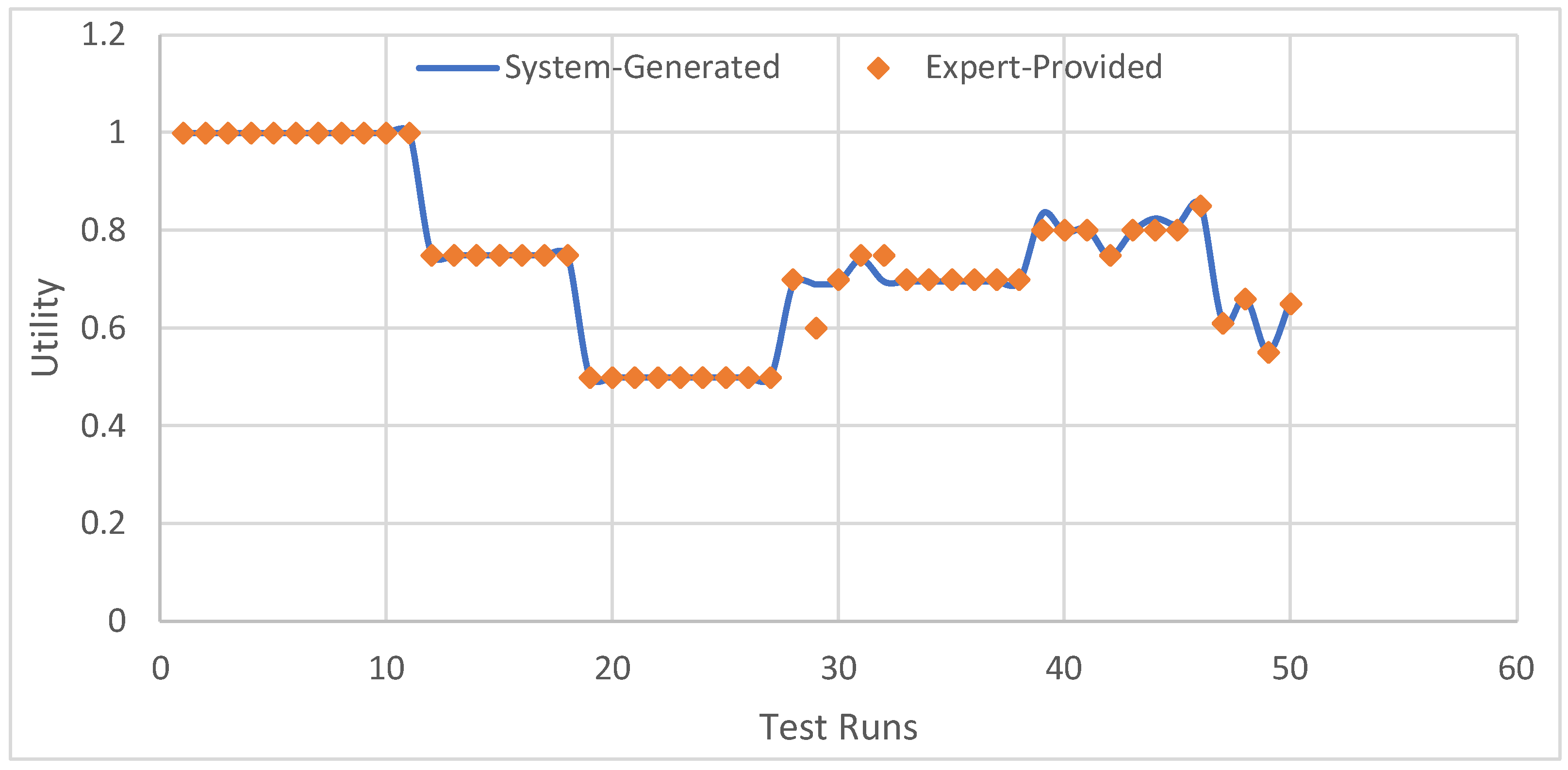
of Appendix A. A scatter chart was used to plot the decision-tool-generated utilities and the expert-provided utilities of the optimal alternatives in Figure 10, to visualize the degree of alignment between the decision tool’s results and the experts’ opinions.

Figure 10 shows that the line for expert-provided utilities largely overlaps with the one for decision-tool-generated utilities for the 50 test runs. This suggests that the proposed decision support correctly selected almost all of the optimal alternatives for the given 50 cases.

To rigorously validate the model output, a paired t-test will be conducted to determine if the two distributions (expert-provided vs. decision-tool-generated utilities) significantly differ from each other. However, before applying this statistical test, a normality test will also be conducted to ensure that both distributions are normally distributed.

3.7.2. Normality Test

The two distributions have been plotted separately in histograms in Figure 11a,b.

To determine if the distributions are bell-shaped, a numerical approach to the normality test is recommended, as it may not be apparent from the histograms (Figure 11a,b). IBM SPSS Statistics version 22 was used to conduct the normality test on both the decision-tool-generated and expert-provided utilities, with 50 tests per 50 cases, as shown in

Table 9. Descriptive statistics of the t-test.

			Statistic	Std. Error
Decision-tool-Generated Utilities	Mean		0.7190	0.02374
	95% Confidence Interval for Mean	Lower Bound	0.6703
		Upper Bound	0.7677
	5% Trimmed Mean		0.7156
	Median		0.6946
	Variance		0.016
	Std. Deviation		0.12562
	Minimum		0.50
	Maximum		1.00
	Range		0.50
	Interquartile Range		0.13
	Skewness		0.279	0.441
	Kurtosis		0.561	0.858
Expert-Provided Utilities	Mean		0.7168	0.02376
	95% Confidence Interval for Mean	Lower Bound	0.6680
		Upper Bound	0.7655
	5% Trimmed Mean		0.7131
	Median		0.7000
	Variance		0.016
	Std. Deviation		0.12573
	Minimum		0.50
	Maximum		1.00
	Range		0.50
	Interquartile Range		0.15
	Skewness		0.258	0.441
	Kurtosis		0.564	0.858

. There were no missing data for this test, as indicated in Table 8. The skewness values for the decision-tool-generated and expert-provided utilities were reported to be 0.279 and 0.258, respectively, both of which fall between −0.5 and 0.5. These values indicate that both datasets are reasonably symmetrical. The kurtosis values were found to be 0.561 and 0.564. A kurtosis value of less than 3 suggests that the tails of the distribution are thinner than in the normal distribution and that the peak of the considered distribution is lower, indicating that the data are light-tailed or lack outliers [64].

3.7.3. Paired t-Test

Since the sample data passed the normality test, a parametric test could be used to validate the decision tool. Therefore, a paired t-test was performed to validate the decision-tool-generated results against the truth data provided by the experts. The results of the paired two-sample t-test are presented in

Table 10. Results of the paired two-sample t-test for means.

	Decision-Tool-Generated Utilities	Expert-Provided Utilities
Mean	0.74764618	0.7464
Variance	0.028370705	0.028460245
Observations	50	50
Pearson Correlation	0.995167299
Hypothesized Mean Difference	0
Df	49
t Stat	0.531646386
P (T <= t) one-tail	0.298686545
t Critical one-tail	1.676550893
P (T <= t) two-tail	0.597373089
t Critical two-tail	2.009575199

. The paired t-test for means yielded a p-value of 0.597, which is greater than the 0.05 significance level. Thus, it can be concluded that there is no statistically significant difference between the decision-tool-generated and expert-provided utilities. It can be inferred that the utilities generated by the decision tool are very similar to the utilities provided by the experts. In the following sections, the performance of the decision tool is rigorously assessed to determine how closely it can emulate a decision-making expert.

3.8. Decision Tool Performance Assessment

The decision tool’s performance has been assessed with the help of three powerful instruments: confusion matrices, the area under the ROC curve, and six other performance metrics.

3.8.1. Confusion Matrices

A confusion matrix is a table that is used to evaluate the performance of a classification model. It compares the predicted class of each sample to its actual class and categorizes them into four different measures: True Positive (TP), True Negative (TN), False Positive (FP), and False Negative (FN) (

Table 11. Confusion matrix structure [65].

Validation	Predicted Positive	Predicted Negative
Actual Positive	True Positive (TP)	False Negative (FN) Type II Error
Actual Negative	False Positive (FP) Type I Error	True Negative (TN)

).

In the context of

Table 12. Confusion matrix for decision tool validation.

	Decision Tool Predicted Alternatives
Expert-Provided Actual Alternatives		A1	A2	A3	A4	A5	A6	A7	A8	A9
	A1	6
	A2		5
	A3			5
	A4				4
	A5					6
	A6						8		1
	A7							3
	A8	1							7
	A9					1				3

, the confusion matrix was used to validate the performance of the proposed tool. It showcases the tool’s predictive capabilities across multiple alternatives (A1–A9) and how they align with expert-provided actual alternatives. This step highlights the tool’s ability to make accurate predictions, forming the foundation for further analysis.

Table 13. Four crucial measures for decision tool validation.

	A1	A2	A3	A4	A5	A6	A7	A8	A9
TP	6	5	5	4	6	8	3	7	3
FP	1	0	0	0	1	0	0	1	0
TN	3	5	5	6	3	1	7	1	6
FN	0	0	0	0	0	1	0	1	1

furthers our understanding by offering a detailed breakdown of True Positives (TP), False Positives (FP), True Negatives (TN), and False Negatives (FN) for each individual alternative. This breakdown not only reveals the tool’s accuracy for each alternative but also uncovers potential areas for improvement, aiding in refining the decision support model.

Table 14. Pooled confusion matrix for decision tool validation.

	Predicted Value
Actual Value		Positive	Negative
	Positive	True Positive (TP) = 47	False Positive (FP) = 3
	Negative	False Negative (FN) = 3	True Negative (TN) = 397

shows the pooled confusion matrix for decision tool validation, where the actual and predicted values are compared across all of the alternatives. The pooled confusion matrix shows that the decision tool predicted 47 True Positives, 3 False Positives, 3 False Negatives, and 397 True Negatives. The pooled confusion matrix allows for an overall evaluation of the decision tool’s performance, showing that it correctly predicted most alternatives, with a low number of false positives and false negatives.

3.8.2. Performance Metrics

Based on the four measures (TP, FP, TN, FN), more meaningful measures of the tool’s performance, such as precision, sensitivity, specificity, accuracy, and F1 score, can be calculated.

$$Precision=\frac{TP}{TP+FP}$$

(20)

$$NegativePredictedValue=\frac{TN}{TN+FN}$$

(21)

$$SensitivityorRecallorTruePositiveRate=\frac{TP}{TP+FN}$$

(22)

$$Specificity=\frac{TN}{TN+FP}$$

(23)

$$Accuracy=\frac{TP+TN}{TP+TN+FP+FN}$$

(24)

According to Mausner et al. [66], a model’s precision determines the number of positive cases that the decision tool correctly identifies out of all of the available positive cases. The negative predicted value of a model reflects how accurately negative cases were classified as negative. Additionally, a model’s sensitivity represents the ratio of correctly identified positive data to the actual positive data, while specificity defines the ratio of correctly classified negative data to the actual negative data. The accuracy measure indicates the percentage of data correctly identified by the model.

Furthermore, the F1 score is a metric that takes into account both the sensitivity and specificity of the model, providing an overall measure of its performance [67].

$$F1ScoreorPerformance=\frac{2\times (Precision\times Recall)}{Precision+Recall}$$

(25)

In

Table 15. Overall model performance measures.

Performance Measure	Value
Precision	$\frac{TP}{TP+FP}=\frac{47}{47+3}=0.94$
Negative Predicted Value	$\frac{TN}{TN+FN}=\frac{397}{397+3}=0.9925$
Sensitivity	$\frac{TP}{TP+FN}=\frac{47}{47+3}=0.94$
Specificity	$\frac{TN}{TN+FP}=\frac{397}{397+3}=0.9925$
Accuracy	$\frac{TP+TN}{TP+TN+FP+FN}=\frac{47+397}{47+397+3+3}=0.9867$
F1 Score	$\frac{2\times (0.94\times 0.94)}{0.94+0.94}=0.94$

, the performance metrics offer a comprehensive assessment of the decision support model’s effectiveness. Precision, negative predicted value, sensitivity, specificity, accuracy, and the F1 score emphasize the tool’s strengths in correctly identifying both positive and negative cases. These metrics, derived from the confusion matrices (Table 14), showcase the decision tool’s well-rounded performance and its potential to contribute effectively to decision-making processes.

The decision support model correctly identified over 99% of negative cases with a negative projected value of 0.9925, and accurately detected 47 out of 50 predicted-positive cases with a sensitivity of 0.94. The specificity of the decision tool was 0.9925 or 99.25%, and the accuracy was 0.9867, indicating that the decision tool can accurately identify over 98% of cases. The F1 score for the proposed decision tool was 0.94, which measures the performance of a decision tool as the harmonic mean of precision and recall. This score further confirms the excellent performance of the decision support tool.

3.8.3. Receiver Operating Characteristics (ROC)

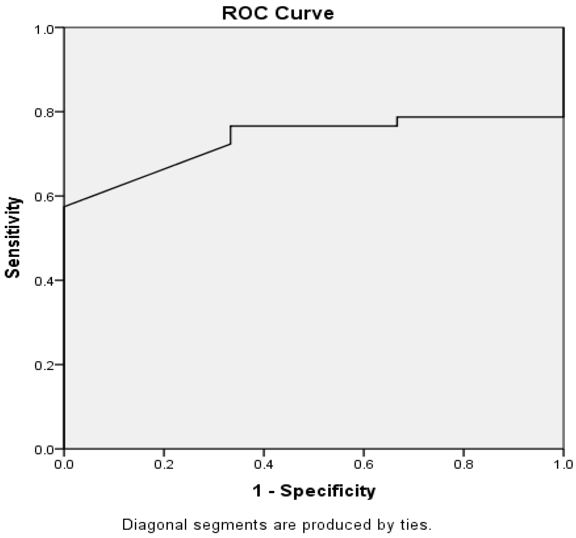
The ROC curve is a visual representation of a model’s performance that helps compare different models with a specific objective. The area under the ROC curve is a common metric used to validate the effectiveness of a classifier. The ROC curve was generated using IBM SPSS V.22, and the area under the curve (AUC) was calculated to better understand the decision tool’s performance. The ROC curve demonstrates the model’s sensitivity against the false positive rate, and the closer the curve is to the left and upper border, the better the model’s performance. The results are presented in

Table 16. Area under the ROC curve for decision-tool-generated utilities.

Area		0.734
Std. Error (under the nonparametric assumption)		0.071
Asymptotic Significance		0.178
Asymptotic 95% Confidence Interval	Lower Bound	0.594
	Upper Bound	0.874

and Figure 12.

The AUC of the proposed decision tool was 0.734, indicating that it performs better than random guessing (AUC = 0.5) but is not a perfect classifier (AUC = 1). The asymptotic significance was 0.178, which is greater than 0.05, suggesting that the developed decision support tool is valid.

4. Discussion, Conclusions and Future Work

Universities worldwide are striving to modernize their traditional campuses and incorporate smart technology. However, implementing a variety of smart applications can leave campus management unsure about the optimal order of implementation and the key success factors and potential benefits. To address this issue, a comprehensive decision-making model has been developed to help a university’s strategic management team to prioritize smart campus solutions based on its specific circumstances.

Previous research has highlighted the importance of smart technologies in various industries, including the potential benefits of smart campuses in the education sector. The current study builds upon this knowledge by proposing a comprehensive decision-making model specifically tailored for universities.

Firstly, through a literature survey, six main objectives were identified: enhancing workflow automation, safety and security, teaching and learning, strategic management, and resource conservation. These objectives are achieved through four underlying technologies: cloud computing, IoT, AR and VR, and AI. Smart campus solutions were grouped into nine functional families through a stakeholder opinion survey, followed by a statistical analysis to ensure clear and non-overlapping grouping of options. This aligns with previous studies that have emphasized the need for smart applications to enhance workflow automation, safety and security, teaching and learning, strategic management, and resource conservation. The integration of cloud computing, IoT, AR and VR, and AI technologies further aligns with the evolving landscape of smart technologies.

Secondly, six critical success factors at the strategic level were identified from the literature, including the three types of costs (implementation, operation, and maintenance), implementation duration, resource availability, and stakeholders’ perceived benefit. These success factors were included as attributes in the multiple criteria decision analysis (MCDA) problem for evaluating each alternative. After reviewing various decision-making frameworks, the evidential reasoning (ER) approach was selected as the most appropriate among 12 surveyed MCDA methods to apply to the smart campus strategic decision problem.

The ER model was established through a mathematical formulation, followed by the Dempster–Shafer algorithm. To determine the relative importance of attributes, a group of experts consisting of faculty, staff, and operational managers utilized the Nominal Group Technique and provided their final voted weights. Subsequently, the ER model was programmed in Python and takes in a three-dimensional tensor of degrees of belief, where each element is a degree of belief at the intersection of an alternative, an attribute, and an evaluation grade. The model outputs the average utility of each alternative and a ranking of alternatives in descending order of average utility, with the optimal alternative being the top-ranked option.

To validate the decision tool, 50 belief tensors were randomly generated and assessed simultaneously through the model and by a group of decision-making experts who provided utilities for each alternative using their experience and judgment. The model’s validity was evaluated using a paired t-test, which indicated no significant difference between the expert-provided and model-generated results, even at the 0.05 significance level. Additionally, the area under the model’s ROC curve was determined to be 0.734, indicating that the model outperformed random guessing. To evaluate the model’s performance, seven metrics were used, including accuracy, precision, sensitivity, specificity, negative predicted value, and F1 score. All metrics were found to be above 90%, highlighting the soundness of the model and its ability to reliably emulate a decision-making expert.

The validation of the ER approach as a highly reliable decision-making tool reinforces the findings and contributes to the broader context of decision support in the implementation of smart solutions. By utilizing expert opinions and comparing the model-generated results with human experts’ assessments, the study demonstrates the tool’s effectiveness in emulating decision-making expertise.

The implications of these findings extend beyond the specific context of the study. The decision-making tool can serve as a generalized tool for worldwide use, helping universities globally make informed decisions about implementing smart campus solutions. This contributes to the modernization of traditional campuses on a global scale and facilitates the adoption of smart technologies in the education sector.

The findings of this research provide valuable insights into the optimization of smart campus solutions through the proposed decision-making tool based on the evidential reasoning (ER) approach. The tool addresses the challenge of prioritizing smart applications based on specific requirements and circumstances of universities. By considering various attributes such as implementation cost, operation cost, maintenance cost, implementation duration, resource availability, and stakeholders’ perceived benefit, the tool provides rankings and utilities for different smart applications.

Although the study successfully achieved its aim, a few limitations and possible areas of improvement were identified:

• When applying the tool to another university campus, the attribute weights should be adjusted to reflect that university’s unique values hierarchy.
• The tool assumes that the university’s leadership is not bound by any strategic commitments, such as sustainability goals, so adding “Strategic Alignment” as an extra attribute to the tool in the future may be useful.
• The tool outlines the digital transformation plan for a fully traditional campus, so if the campus has already incorporated some smart applications, the decision-making tool must consider these existing systems by excluding them from the alternatives.
• Implicit costs, such as opportunity cost, are not accounted for in the tool, so investigating how to incorporate them would be interesting.
• The tool currently does not prompt the user for the institution’s budget, which means that an alternative that exceeds the budget would not be excluded from the analysis, but a simple mechanism could be implemented to automatically exclude alternatives with annualized costs that exceed the budget.
• The evaluation of cost is left to subjective interpretation, so establishing more objective and concrete definitions of cost would be helpful.
• To increase the tool’s resolution, more evaluation grades can be added, such as “Excellent”, “Very Good”, “Good”, “Average”, “Below Average”, “Bad”, and “Very Poor”, or a continuous utility function can be assumed, but this may negatively impact user experience.
• Expanding the tool’s scope by including other important factors, such as social impact, environmental impact, and ethical considerations, to help universities make more socially responsible and sustainable decisions.
• Collaborating with other universities to gather more data and insights on their smart campus implementation strategies and to better understand the variations in universities’ priorities and values.
• Investigating the applicability of the developed tool to other industries, such as healthcare or manufacturing, to see if the tool can be adapted for other decision-making contexts.

This study has developed a comprehensive decision-making model that addresses the challenge of prioritizing smart applications in universities. The validation of the model confirms its reliability and effectiveness, and its generalizability enables universities worldwide to make informed decisions about implementing smart campus solutions. The identified limitations and potential areas for improvement offer valuable directions for future research, enhancing the tool’s usability, objectivity, and applicability across various contexts.