Dynamic Pricing for Charging of EVs with Monte Carlo Tree Search

Abstract

As electric vehicles (EVs) are slowly becoming a common occurrence on roads, commercial EV charging is becoming a standard commercial service. With this development, charging station operators are looking for ways to make their charging services more profitable or allocate the available resources optimally. Dynamic pricing is a proven technique to increase revenue in markets with heterogeneous demand. This paper proposes a Markov Decision Process (MDP)-based approach to revenue- or utilization- maximizing dynamic pricing for charging station operators. We implement the method using a Monte Carlo Tree Search (MCTS) algorithm and evaluate it in simulation using a range of problem instances based on a real-world dataset of EV charging sessions. We show that our approach provides near-optimal pricing decisions in milliseconds for large-scale problems, significantly increasing revenue or utilization over the flat-rate baseline under a range of parameters.

1. Introduction

1.1. Motivation

After more than a hundred years of niche use, electric vehicles (EVs) seem on the cusp of displacing internal combustion engine (ICE) vehicles in personal transportation [1,2]. Better fuel efficiency, environmental friendliness, and lowering costs give EVs an edge over ICE vehicles. To this end, the authors in [3] reported that in 2020 there was an increase of EVs from 3.5% to 11% of total new car registrations.

The rise of EVs drives interest from many different actors, including governments, cities, car manufacturers, environmental groups, and electric utilities. Each is trying to prepare for the expected rise of EVs. For cities and electric utilities, the widespread use of EVs may require significant investments into infrastructure, as large numbers of EVs could increase the peak load on the grid up to threefold [4]. Thus, demand-side management (DSM) methods such as peak load shedding and valley filling allow for moving the demand of customers from peak times (e.g., noon) to off-peak times (e.g., early morning), which prevents the infrastructure costs from growing.

This concern for future infrastructure investment is one of the primary motivations for the recent interest in dynamic pricing. For this reason, different fields such as economics, revenue, or supply chain management study dynamic pricing as a technique to balance the demand in various domains [5,6]. In the field of smart mobility, where we do not assume centralized control, authors of [7] propose dynamic pricing to improve the efficiency of taxi systems while [8,9,10] use dynamic pricing to help with power grid management in electric mobility, balancing demand, power quality, and other grid-related metrics. These fields recognize dynamic pricing as a critical lever for influencing buyers’ behavior. Hence, in this paper, we propose a dynamic pricing scheme to deal with increasing loads on the charging stations caused by the uptake of EVs.

Until recently, most research on charging for electric vehicles focused on optimizing charging station placement [11,12,13,14,15,16]. Such approaches are only a seeming remedy in a changing environment where charging station placement is no longer optimal in the new environment. On the other hand, the dynamic pricing of EV charging and its application to load balancing is robust to the dynamically changing situation in the infrastructure, demand, and energy costs. This direction was taken by, e.g., Xiong et al. [17]. The proposed pricing problem considers EV drivers’ travel patterns and self-interested charging behavior. Authors view the problem as a variation on sequential posted pricing [18] for charging stations and propose a mixed-integer nonconvex optimization of social welfare in the model.

Dynamic pricing of EV charging is a method that can potentially provide a cheap and robust alternative to expensive upgrades of the current grid infrastructure. However, the applications proposed above focus on dynamic pricing primarily toward optimizing the social welfare function. Yet, in real-world situations, prospective charging station (CS) operators are often privately owned and not strongly incentivized to improve social welfare. Instead, private investors are concerned with the costs of installing and providing charging services and their financial returns (From report “An Industry Study on Electric Vehicle Adoption in Hong Kong” by the Hong Kong Productivity Council (2014): www.hkpc.org/images/stories/corp_info/hkpc_pub/evstudyreport.pdf (accessed on 7 February 2022)).

1.2. Problem Statement and Contributions

This paper studies the problem of allocating EV charging capacity using a dynamic pricing scheme. We focus on (1) maximizing the revenue of the CS operator and (2) maximizing the overall utilization of the corresponding charging station. To formulate the pricing problem, we apply the Markov Decision Process (MDP) methodology [19].

To derive the optimal solution of the small instances of the MDP problem, we can use exact solution methods such as value iteration (VI), policy iteration, or integer linear programming. However, all these methods suffer from the state-space explosion problems due to the large-scale nature of the real-world environment. We use a Monte Carlo Tree Search (MCTS) heuristic solver to approximate the optimal pricing policy to remedy this problem. This is the first usage of MCTS in this kind of problem to the best of our knowledge. Consequently, we contribute to the body of research by applying the theory to the real-world problem of dynamic pricing of EV charging suitable for electric mobility.

Some of our key contributions are:

• Novel model of dynamic pricing of EV charging problem using the Markov Decision Process (MDP) methodology;
• A heuristics-based pricing strategy based on Monte Carlo Tree Search (MCTS), which is suitable for large-scale setups;
• Optimizations based on maximizing the revenue of the CS operators or the utilization of the available capacity;
• Parametric set of problem instances modeled on a real-world data from a German CS operator which spans two years;
• Experimental results showing that the proposed heuristics-based approach is comparable to the exact methods such as Value Iteration. However, unlike those exact methods, the proposed heuristics-based approach can generate results for large-scale setups without suffering from the state-space explosion problem.

We organize the rest of the paper as follows: In Section 2, we list the different contributions in the literature which consider the problem of online session-based dynamic pricing of the EV charging problem. We give the MDP formulation of the problem under study in Section 3. We introduce the proposed heuristic based on MCTS in Section 4. Then, we describe the different considered baseline pricing methods such as the flat rate, our proposed MCTS method, optimal VI pricing, and oracle-based upper bound baseline, and  compare the underlying experimental results in Section 5. We conclude the paper in Section 6, giving future research directions.

2. Related Work

Price- as well as incentive-based schemes, are promising techniques to realize demand-side management (DSM). The price-based DSM encourages end-users to change their demand (e.g., load) in response to changes in electricity prices. On the other hand, incentive-based DSM gives end-users load modification incentives that are separated from, or in addition to, their retail electricity rates. This paper adopts the price-based scheme for the problem under study.

The field of energy systems has proposed several price-based schemes, such as time-of-use (ToU) [20], real-time pricing (RTP) [21], and critical-peak pricing (CPP) [22]. These schemes, as mentioned above, change the load of the end-users by considering the needs of energy suppliers. To this end, the prices increase during peak demand and decrease during the surplus of generation, e.g., from renewables. Building on the three pricing schemes mentioned above, recently another method was proposed, known as dynamic pricing [23].

To put dynamic pricing into perspective, we can see it as the pricing of services in high demand or that each buyer values differently, such as hotel rooms [24] or airline tickets [25]. For airfares and hotel rooms, the price is changing based on the expected demand throughout the season, existing bookings, and the customer’s segment (business or tourist). Services such as airfares and hotel rooms have a strict expiration deadline: the departure of the airplane and the arrival of the booked day. Similarly, the EV charging resources in a given time window expire if there are no vehicles to use them. With such a type of perishable service, the goal is to sell the available service capacity for profit under the constraints given by their expiration and fluctuations in demand. Unused service capacity is a wasted profit opportunity for CS operators. Maximizing revenue from these expiring services is the topic of revenue management [6].

For the seamless integration of renewable energy sources and EVs into the power grid, dynamic pricing schemes have been proposed in the literature. In this respect, the different contributions in the literature can be further classified into price-profile- and session-based methods. The former approaches set different prices for EV charging based on different time intervals, whereas the latter specifies one price for the whole duration of the charging session. In  is paper, we adopt the session-based pricing method. Next, we introduce session-based approaches proposed in the literature.

In [26], the authors use the queuing theory methodology to study the performance of charging stations by dynamically changing the prices so that the overall throughput is maximized and the waiting time is minimized. The authors in [27] use the game theory methodology in general, specifically the Vickrey–Clarke–Groves (VCG) auction mechanism, to specify prices for charging sessions such that the social welfare function is maximized. It is important to note that in such auction-based approaches, two or more EV users are charged differently despite having the same charging duration, arrival time, and charging demand (e.g., total energy).

From the perspective of realization, there are different types of contributions in the literature, categorized into offline and online approaches. The former method specifies charging prices for extended time periods (e.g., one day) based on some information related to the projected EV charging demand, such as the number of EVs to be charged during this period, their required charging amount, etc. On the other hand, online approaches specify charging prices for short periods and often update them. This is the line of research that this paper is adopting. In this respect, several contributions can be found in the literature. Like our approach, in [28] the authors assume that the charging prices change dynamically, and the EV users are offered different prices on a session basis. The EV users can either accept or reject the proposed price. The authors also suggest that the CS operator has to pay some penalties in case the waiting time of the EV users exceeds a certain threshold. The proposed scheduling algorithm has the main objective of maximizing the profit of the CS operators. In [29], the authors also consider the problem of optimally allocating the charging stations’ capacity to maximize the CS operators’ profit. To this end, they propose a framework that changes the price of charging dynamically so that the EV users can either accept or reject the offered price. Consequently, the framework can also be used to minimize the number of rejections by EV users.

In this paper, we consider the dynamic pricing of EV charging using online and session-based techniques. However, unlike the contributions above, the underlying problem under study is formulated using the Markov Decision Process (MDP) methodology. We base our model on the MDP pricing model introduced in [30], but significantly improves how we model historical charging demand. We also managed to solve much larger problem instances thanks to the proposed MCTS method. To the best of our knowledge, this is the first attempt to apply MCTS to the dynamic pricing of EV charging.

3. MDP Formulation of EV Dynamic Pricing Problem

In this section, we describe our dynamic pricing model and its formalization in the Markov Decision Processes (MDPs) framework [19].

Our dynamic pricing model assumes (1) a monopolistic seller, which is a charging station (CS) operator, and (2) non-strategic customers, which are the electric vehicle (EV) users. At any point in time, the CS operator has limited available charging capacity to charge several EVs simultaneously. This operator’s objective is to sell the available charging capacity to the EV users while optimizing some criteria (e.g., revenue or utilization).

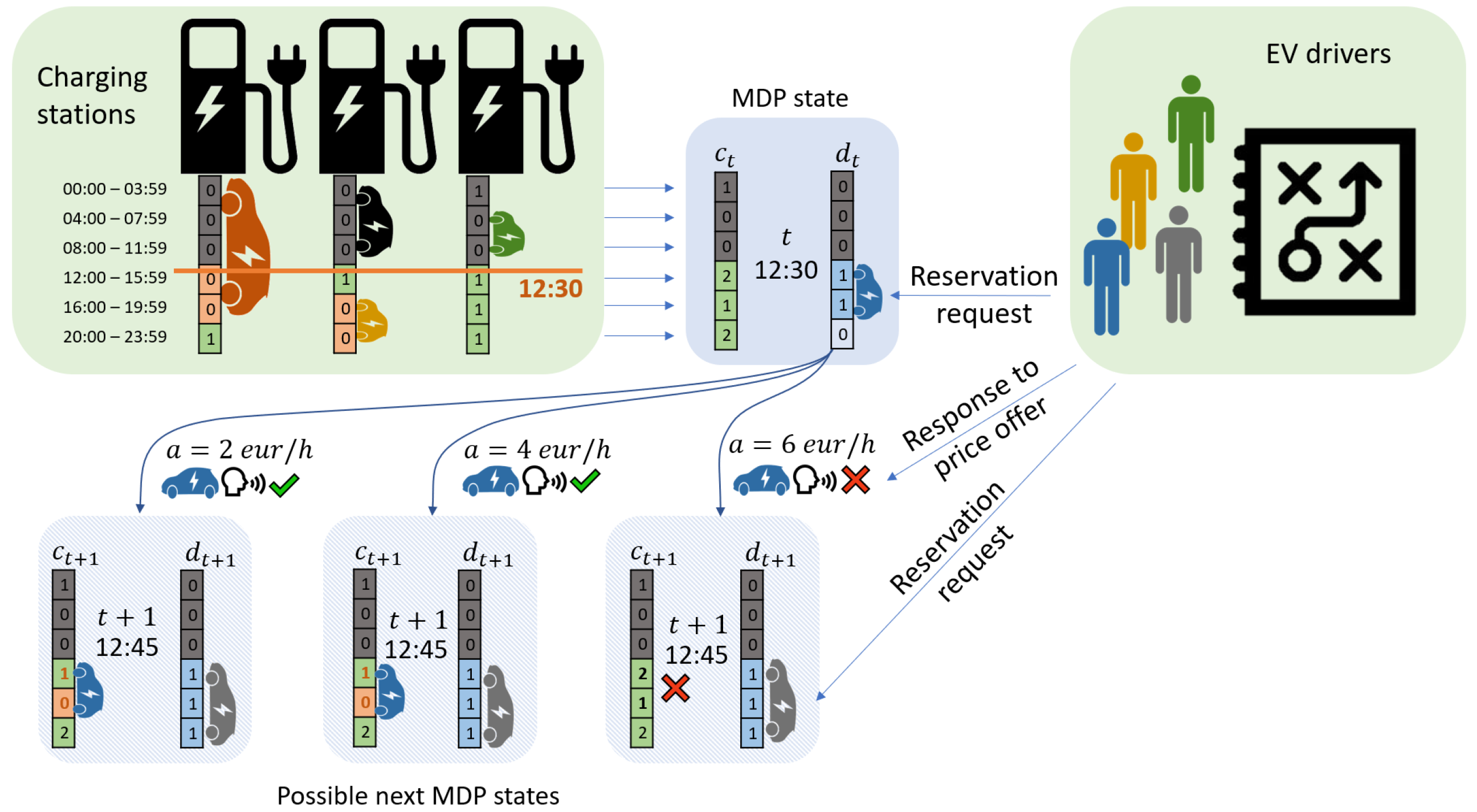
During the day, the CS operator receives a sequence of EV charging requests in the form of reservations of future charging capacity [31,32]. The operator prices each request according to some pricing policy. It is up to the EV user to either accept (e.g., the green tick sign in Figure 1) or reject (e.g., the red cross sign in Figure 1) the offered price. If the EV user accepts the price, the CS operator assigns the reserved charging capacity to this user. If the user rejects the price, the charging capacity remains available for the following requests. As such, this is a sequential, online session-based dynamic pricing problem.

The major challenge for the CS operator is the fact that to allocate the requested capacity optimally, the CS operator would need to know:

• which reservations will arrive during the day,
• what will be the EV user’s responses to the offered prices.

However, the CS operator does can not get this information directly. Nevertheless, using historical data, the CS operator can probabilistically model the reservation arrivals and EV user responses to prices. Thus, the CS operator can optimize his actions in  expectation.

3.1. MDP Formalization

MDPs provide a model for decision-making problems under uncertainty, with solutions either optimal or converging to optimal in expectation (with respect to the probability distributions involved). MDPs are defined by the tuple $(S,A,\tau ,R)$, where S is the set of states, $\tau$ is the transition function, R is the reward function and A is the set of available actions. For the dynamic pricing of the EV charging problem under study, we will describe these four components separately.

3.1.1. State Space

The state-space S consists of states $s=(\mathit{c},t,\mathit{d})$ (sometimes, we also use $s_t=(\mathit{c},\mathit{d})$ to denote a state at t). That is, the state is defined by the available capacity vector $\mathit{c}$ at time t and the charging session $\mathit{d}$ being requested by some customer at t. Figure 1 gives a graphical presentation of the considered states of the MDP. Note that among those three state variables, t represents the “wall clock” of the seller (e.g., CS operator). We use discretized timesteps for $t\in \mathbb{N}$ and a finite time horizon of one day, thus leading to the fact that the number of timesteps T is finite (e.g., for a timestep of 15 min, this results in 96 timesteps in one day).

The day is also discretized into EV charging timeslots. Each timeslot represents a unit of charging (e.g., in Figure 1 each timeslot is 4 h). The vector $\mathit{c}\in {\mathbb{N}}^K$ represents the available charging capacity in each of K timeslot of a given day. Note that the number of timeslots K is much lower than the number of timesteps T, $K<<T$ (e.g., in Figure 1, $K=6<<T=96$).

Finally, $\mathit{d}$ is a vector representing a charging session some EV user is trying to reserve. The vector has the same dimension as the capacity vector, so $\mathit{d}\in {\left[0,1\right]}^K$, but its values are binary, 1 meaning the EV user wants to charge in a given timeslot, 0 otherwise.

The size of the whole state-space is then $T{c}_0^K{2}^K$, where $c_0$ is the initial capacity in all timeslots. It can be noticed that for a limited number of EV users and charging stations, the number of MDP states increases exponentially with the number of timeslots, leading to state-space explosion problems for exact closed-form solution methods such as VI or ILP.

3.1.2. Action Space

The action space A is a set of possible prices (per hour of charging) that the CS operator can offer to the EV users. We assume a finite set of prices, spread evenly over the support of the user budget distribution, with twice as many price levels as there are charging timeslots, $\left|A\right|=2K$.

3.1.3. Reward Function

The reward function $R(s_t,a,s_{t+1})$ determines the reward obtained by transitioning from state $s_t$ to state $s_{t+1}$ by taking action (offering price) a. If the optimization goal is revenue maximization of the CS operator, then reward is the accepted price by the EV user, $R(s_t,a,s_{t+1})=a$ or 0 if the EV user rejects the offer. If the goal is maximizing utilization (e.g., a number between 0 (no charging sessions served) and 1 (all timeslots in a day are utilized)), the reward in case the EV user accepts the proposed price would be the percentage of the used capacity, $R(s_t,a,s_{t+1})={\left|\mathit{d}\right|}_1/{\left|{\mathit{c}}_0\right|}_1$, where ${\left|\mathit{d}\right|}_1$ is the sum of the elements of a vector $\mathit{d}$. Different utility functions will lead to significantly different pricing policies, and any utility function that can be expressed as dependent on the MDP state transitions can be used.

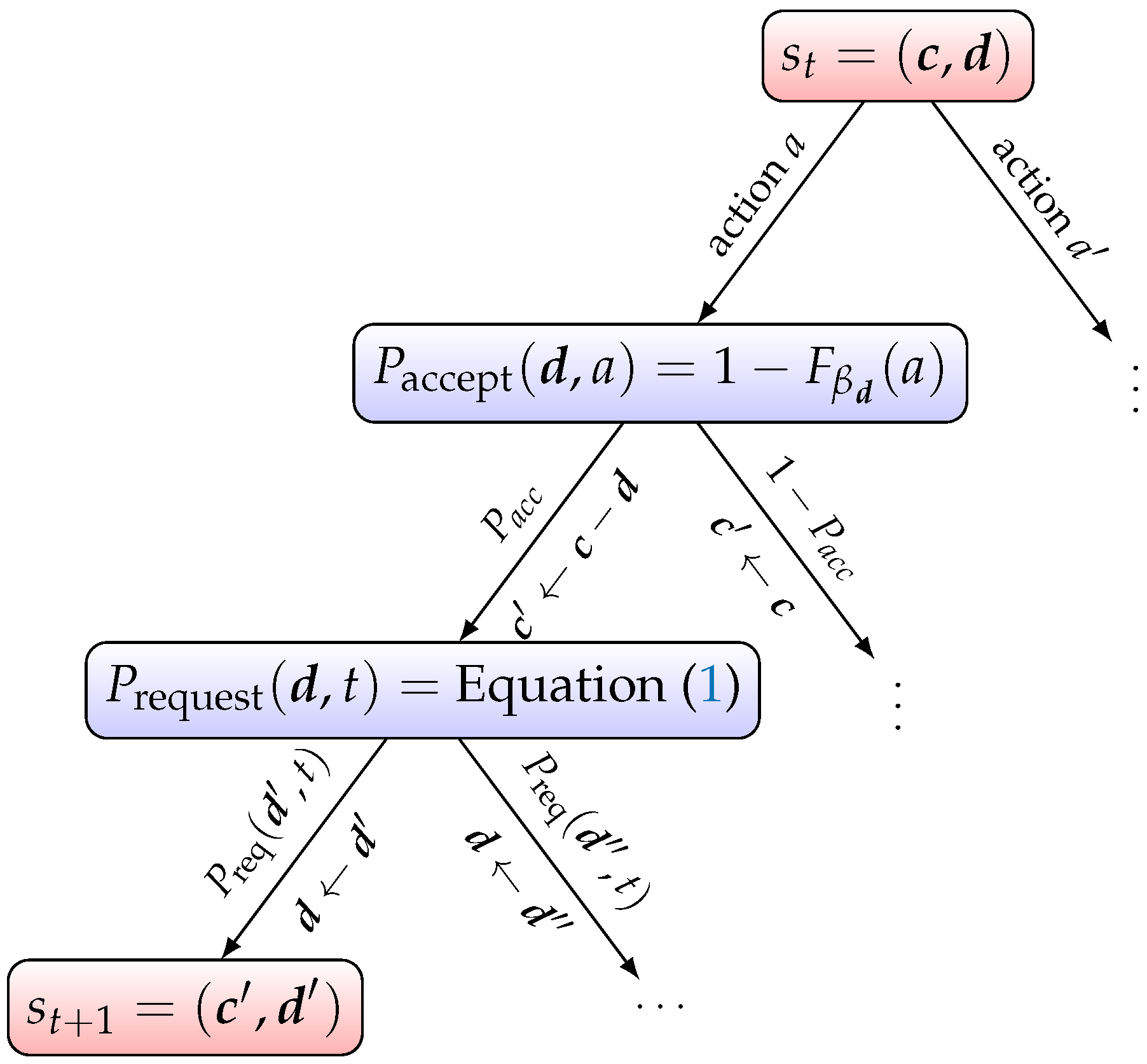
Transition function $\tau$ determines the MDP reward by following the tree edges in Figure 2 from the root to a leaf. Within the reward function, the EV user’s acceptance is observed by comparing $\mathit{c}$ between two consecutive states for t and $t+1$. If the capacity is reduced between $s_t$ and $s_{t+1}$, then this indicates that the EV user has accepted the CS operator’s price otherwise it is rejected. Formally (showing only the case of revenue maximization):

$$R(s_t,a,s_{t+1})=\left\{\begin{array}{cc}a,\hfill & \mathrm{if} {\mathit{c}}_{t+1}={\mathit{c}}_t-{\mathit{d}}_t\hfill \\ 0,\hfill & \mathrm{otherwise}\hfill \end{array}\right.$$

3.1.4. Transition Function

The transition function $\tau (s_t,a,s_{t+1})$ captures the probability of getting from state $s_t$ to state $s_{t+1}$ via action a. In our case, it is a combination of the charging reservation arrival processes and the EV users’ budget distributions. To this end, the reservation arrivals to the CS operator are modeled using Poisson processes (a common choice in the literature [33,34]), one for each possible charging session $\mathit{d}$ such that it has an arrival rate (e.g., intensity) of ${\lambda }_{\mathit{d}}$. Briefly, a Poisson process for arrivals is one in which those arrivals are identically and independently distributed (IID) such that the inter-arrival times (time between two arrivals) are exponentially distributed.

The probability of some charging session $\mathit{d}$ being requested at timestep t is obtained from the discretized Poisson processes of reservation arrivals. In the case of discrete timesteps, the total number of requests $N_{\mathit{d}}$ for the charging session $\mathit{d}$ approximately follows the binomial distribution with expected value $\mathbf{E}\left(N_{\mathit{d}}\right))=P_{request}\left(\mathit{d}\right)T_{\mathit{d}}$, where $T_{\mathit{d}}$ is the number of timesteps during which the charging session $\mathit{d}$ could possibly be sold, and $P_{request}\left(\mathit{d}\right)$ is the probability of charging session $\mathit{d}$ being requested at any point between timestep 0 and $T_{\mathit{d}}$. We then define the probability of any charging session request at timestep t as:

$$P_{request}(\mathit{d},t)=\left\{\begin{array}{cc}{P}_{request}\left(\mathit{d}\right),\hfill & \mathit{d}\in D\mathrm{s}.\mathrm{t}.t<T_{\mathit{d}}\hfill \\ 1-{\displaystyle \sum _{\mathit{d}\in D\mathrm{s}.\mathrm{t}.t<T_{\mathit{d}}}}{P}_{request}\left(\mathit{d}\right),\hfill & \mathit{d}=⌀\hfill \end{array}\right.$$

(1)

where the second case corresponds to no charging session requested at timestep t.

Given the observed demand for charging session $\mathit{d}$, $N_{\mathit{d}}$, we approximate the probability $P_{request}\left(\mathit{d}\right)$ as $P_{request}\left(\mathit{d}\right)=N_{\mathit{d}}/T_{\mathit{d}}$, where we have to select the time discretization fine enough so that $P_{request}\left(\mathit{d}\right)\ll 1$. This is done to keep the approximation error caused by the timestep discretization low.

In our model, the selling period for every possible charging session starts at timestep 0, corresponding to the start of the day, and ends at some timestep $T_{\mathit{d}}$, but the latest at the end of the day, on timestep T. In case an EV charging reservation arrives in timestep t, the probability of an EV user accepting the offered price a for charging session $\mathit{d}$ is given by the cumulative density function of the budget distribution ${\beta }_{\mathit{d}}$ as

$$P_{accept}(\mathit{d},a)=1-F_{{\beta }_{\mathit{d}}}\left(a\right)$$

(2)

The two components of the transition function, $P_{accept}(\mathit{d},a)$ and $P_{request}(\mathit{d},t)$ are multiplied with each other according to Figure 2 to obtain the transition probability $\tau (s_t,a,s_{t+1})$.

In Figure 2, in the root, we have $\left|A\right|$ available actions leading to a binary accept or reject decision on the second level. This decision determines whether the capacity is reduced to $c^{\prime }$ in $s_{t+1}$ or whether it remains the same. In the third level, one of the $|{\left[0,1\right]}^K|$ possible charging sessions (including no charging session) can be requested, determining the next value of $\mathit{d}$ in $s_{t+1}$. Consequently, the maximal branching factor for some state $s_t$ is $2^{K+1}$, K being the number of timeslots.

In the decision tree in Figure 2, note that the chance node with $P_{accept}(\mathit{d},a)$ comes before the node with $P_{request}(\mathit{d},t)$, and not the other way around. This is because first, we determine whether our selected action a will result in EV user acceptance of the requested product $\mathit{d}$. Then we determine which charging session ${\mathit{d}}^{\prime }$ will be requested in the next state.

3.2. MDP Solution

The solution to the above described MDP is a pricing policy, mapping from the state-space S to the action space A. An optimal solution is a pricing policy that maximizes the expected utility with respect to the transition function. In our case, we consider the utility function to be either revenue for the CS operator or the utilization of the CS capacity.

4. Optimal and Heuristic Solutions

This section describes the methods we use to derive the dynamic pricing policies. First, we briefly discuss Value Iteration (VI), an offline method for solving MDPs that converges to an optimal policy. Then, we describe the Monte Carlo Tree Search (MCTS) solver, an online randomized heuristic method that approximates the best actions from any state.

VI is a simple yet accurate method for solving MDPs that converges to an optimal policy for any initialization. The advantage of VI is that it quickly converges to a complete near-optimal pricing policy at the cost of enumerating the whole state-space in memory. Since the state-space size is $T{c}_0^K{2}^K$, this gives VI an exponential space complexity in the number of timeslots. Thus, it does not scale well to larger problem instances. We use VI only to obtain optimal policies on smaller problem instances to validate the heuristic approach of MCTS. Note that there are other exact solution methods for MDP problems than VI, such as policy iteration or linear programming. All these methods can provide the same optimal pricing policy as VI. However, just as VI, all these methods require enumeration of the whole state-space. Our choice of VI is therefore arbitrary.

Our solution method of choice for large-scale problems is MCTS. Unlike VI, MCTS does not need to enumerate the whole state-space. Instead, it looks for the best action from the current state and expands only states that the system is likely to develop into. However, unlike VI, for every state, MCTS only approximates best actions. MCTS improves its approximations of best action with the number of iterations.

Nonetheless, it can be stopped at any time to provide currently the best approximation of optimal action. These properties make it a helpful methodology in dynamic pricing. With MCTS, we can apply changes in the environment to the solver quickly. Even in large systems, the price offer can be generated quickly enough for a reasonable response time to customers. To the best of our knowledge, this is the first attempt to solve the EV charging dynamic pricing problem using MDP and MCTS.

VI is an offline method, where most of the computation happens before the execution of the pricing policy. Applying the policy during the execution consists of simply looking up the best action in the policy data structure. MCTS does not prepare the pricing policy beforehand. On the contrary, the best action for a given state is estimated during the execution. MCTS, therefore, requires more computational resources to execute than VI.

In general, MCTS [35] is a family of methods that use four repeating steps to determine the best action in some state s. Given a decision tree rooted in s, a tree policy is used to traverse the tree until some node $s^{\prime }$ is selected for expansion and a new leaf node is added to the tree. The value function of the new node is estimated by a rollout that quickly simulates transitions from $s^{\prime }$ until a terminal state using a random rollout policy. The accumulated reward from the rollout is then backpropagated to the nodes of the decision tree.

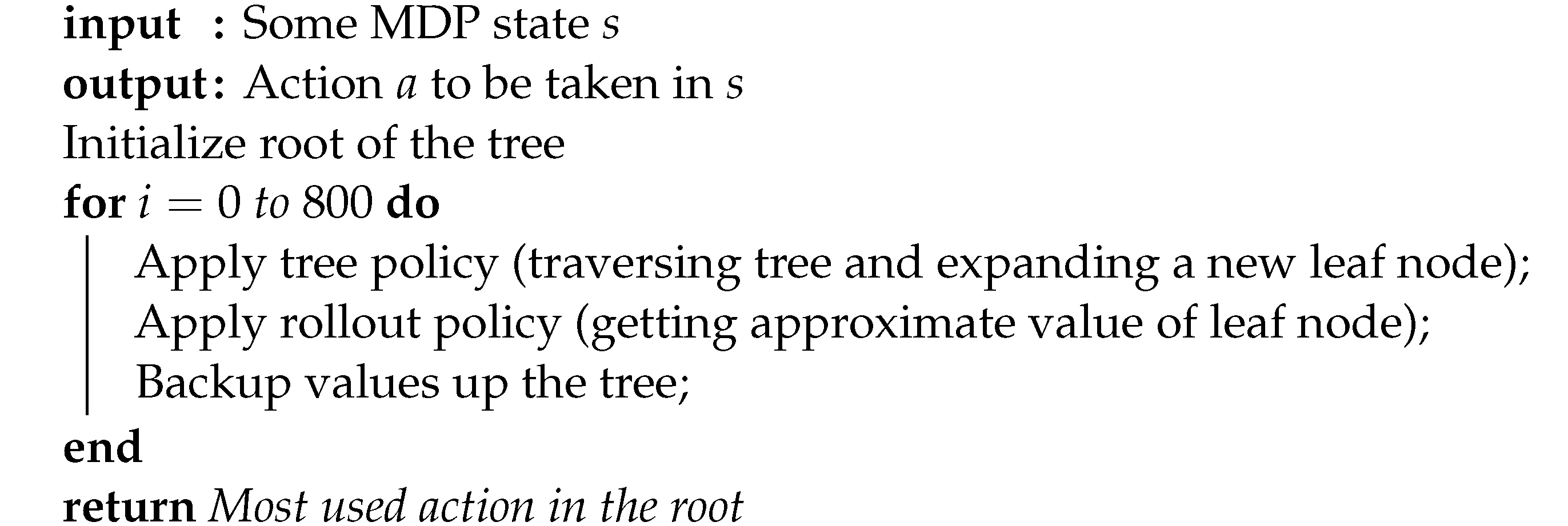
The number of iterations of this selection—expansion—rollout—backpropagation loop is repeated until the predetermined time limit or the required number of iterations. Usually, the higher the number, the closer the resulting action is to the optimum. The general pseudo code of the MCTS is given in Algorithm 1. Our MCTS algorithm is based on a Julia MCTS implementation [36].

Algorithm 1: General MCTS structure.

4.1. Tree Policy

An important part of the algorithm is the tree policy that determines the traversal of the tree and which nodes are added to the tree. In our MCTS implementation, we use the popular Upper Confidence-bound for Trees (UCT) variant of MCTS [37,38,39] that treats each node as a bandit problem and uses the upper confidence bound formula to make the exploration-exploitation trade-off between traversing the existing decision tree and expanding a new node from the current state. See [35] for a description of the tree policy. Our experiments construct the tree only until maximum depth 3 with exploration constant 1. For each leaf node, we estimate its value using random rollouts.

4.2. Rollout Policy

The next part of MCTS is the rollout policy. It is applied from the leaf nodes expanded in the tree policy and is used to get an expected reward estimate of the leaf node. Our experiments use the uniformly random rollout policy that applies random actions from the leaf node until a terminal state in the MDP is reached.

Because we approximate the customer arrival processes as a Poisson process (Bernoulli processes after discretization), we can speed up the rollout by sampling the time to the next arrival from the interarrival distribution (exponential or geometric, respectively). We can arrive at the terminal state in fewer steps by doing this. In the last step of the MCTS, the reward accumulated from the rollouts is then backed up, updating the relevant tree nodes. In our experiments, we reuse the decision trees between the steps of the experiments, which improves the speed of convergence. Our experiments’ number of tree traversals and rollouts is set to 800.

5. Experiments and Results

This section presents the experiments carried out with the proposed MDP-based pricing model and MCTS solver described in the previous sections. We compare our solutions against multiple baselines on artificially generated problem instances modeled on a real-life charging station dataset.

The pricing methods are evaluated on EV user charging requests sequences during one day, from 00:00 to 23:59. These sequences take the form of tuples:

$$B_i=(({\mathit{d}}_1,t_1,b_1),({\mathit{d}}_2,t_2,b_2),\dots ),i\in 1\dots N$$

(3)

where ${\mathit{d}}_i,t_i,b_i$ are the EV user charging requests, indexed by their order in the sequence.

While the requested charging session ${\mathit{d}}_i$ and request timestep $t_i$ are sampled from the demand process described by Equation (1), the user budget value $b_i$ is sampled from the user budget distribution for a given charging session, ${\beta }_{\mathit{d}}$.

We apply each pricing method to these sequences and measure the resource usage and revenue at the end of the day. The requests are provided to the pricing method one by one, starting from the earliest request. The method provides a pricing action, and we record the EV user’s response, reducing the available charging capacity if the corresponding user accepts the price. At the end of the sequence, we record the metrics.

5.1. Evaluation Methodology

The best way to evaluate dynamic pricing methods is to deploy them in a real-world setting and compare their performance with non-dynamic pricing strategies. This approach is rarely feasible in the research setting as it requires the opportunity to experiment with real consumers using real products.

Additionally, directly comparing the performance of our method with other dynamic pricing methods is difficult because all published, readily accessible dynamic pricing methods have known to use restrictive assumptions on the underlying problem or incompatible models and generally are not as flexible as the MCTS-MDP-based approach. For example, although the approximate dynamic programming solution proposed in [40] can provide optimal pricing solutions in large problem instances, it only does so with restrictive assumptions on the problem, such as allowing for linear demand models. Another issue is that there are no established benchmark datasets for comparing the performance of dynamic pricing strategies so far. That said, we can still obtain valuable insights into the performance of our Monte Carlo Tree Search heuristics-based pricing algorithm by comparing it to well-defined baseline methods.

5.2. Baseline Methods

Because of the difficulties of evaluating the dynamic pricing policies, we evaluate our proposed MCTS solution against three baseline methods: flat-rate, MDP-optimal VI and oracle. The flat rate represents a lower bound on revenue. The VI baseline returns an optimal pricing policy and represents the best possible pricing method for MDP parameters. Finally, the oracle policy represents the best possible allocation if the CS operator has a perfect knowledge of future requests and EV users’ budgets, which is unrealistic in real-world use cases.

5.2.1. Flat-Rate

The flat-rate policy does not adjust the price of charging sessions. It uses a single flat price per minute of charging for all charging requests. The flat price is based on training request sequences sampled from the problem instance. The price is set to maximize the average utility function across all training sequences. The resulting flat-rate price is then used on the testing simulation runs. We use 25 randomly selected sequences for the training set out of the 100 used in the evaluation.

5.2.2. Value Iteration

The optimal MDP policy generated by a VI algorithm is our second baseline pricing method. This pricing policy is optimal in expectation with respect to the transition probabilities defined in the MDP model. However, the VI does not scale to larger problem instances as it needs to maintain a value for every state. It can therefore only be used for the evaluation of small problem instances. To obtain the VI baseline, we solve the MDP with a standard VI algorithm (https://github.com/JuliaPOMDP/DiscreteValueIteration.jl (accessed on 7 February 2022)). The resulting policy ${\pi }_{\mathrm{vi}}^{*}$ is the policy used in the experiments to determine the pricing actions.

5.2.3. Oracle

Finally, we compare our MCTS-based pricing method against the oracle baseline strategy. Unlike other pricing strategies, oracle is not a practically applicable pricing strategy. It requires the knowledge of the whole request sequence and EV users’ budgets to determine prices. Oracle maximizes the optimization metric to provide a theoretical upper bound on the revenue and resource usage achievable by any pricing-based allocation strategy using this knowledge.

For kth sequence of charging requests $B_k$ with requests indexed by i, the optimum revenue is the result of a simple binary integer program:

$$\begin{array}{ccc}\hfill \mathrm{maximize}& {\displaystyle \sum _{i\in \{1\dots |B_k\left|\right\}}{x}_i{\lfloor b_i\rfloor }_A}\hfill & \hfill \end{array}$$

(4)

$$\begin{array}{ccc}\hfill \mathrm{subjectto}& {\displaystyle \sum _{i\in \{1\dots |B_k\left|\right\}}{x}_i{\mathit{d}}_i^j\le {\mathit{c}}_0^j}\hfill & \hfill j=1,...,\left|R\right|\\ \hfill & x_i\in \{0,1\}\hfill & \hfill i=1,...,|B_k|.\end{array}$$

(5)

where, $x_i$ are the binary decision variables that determine which requests from $B_k$ are accepted by the CS operator. In the objective function (4), the term ${\lfloor b_i\rfloor }_A={max}_{a\in A,a\le b_i}a$ denotes the fact that the budget values in the sequence $B_k$ are mapped to the closest lower values in the action space A. Conditions (5) mean that the accepted charging sessions have to use fewer resources than the initial supply ${\mathit{c}}_0$. We solve the above optimization problem with an off-the-shelf mathematical optimization toolbox [41].

5.3. Problem Instances and EV Charging Dataset

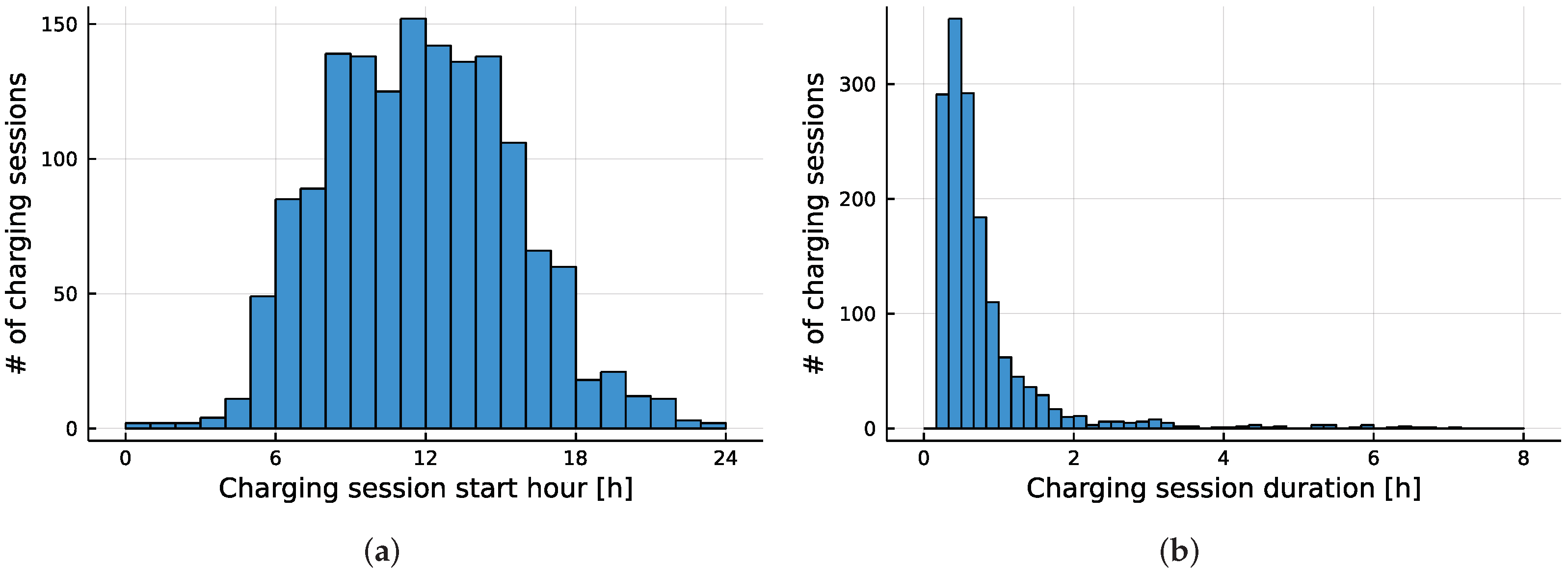
Our experiments consider multiple parametric problem instances based on a dataset of EV charging sessions from a charging location in Germany. After cleaning and preprocessing, the dataset contains 1513 charging sessions spanning over two years. The preprocessing of the dataset consists of removing mostly erroneous charging sessions lasting below 10 min and merging consecutive charging sessions made by the same EV user. These were symptoms of incorrectly plugged charging cables in most of these cases.

Figure 3 shows the histograms of the start time and duration of the charging sessions contained in the dataset. For our problem instances, we approximate these histograms using normal distribution and exponential distribution, respectively. In the dataset, the start times and duration appear uncorrelated (Pearson’s correlation coefficient $=0.008$), so we assume these distributions to be independent. For more details about calculating the Pearson’s correlation coefficient, the interested readers can refer [42]. Furthermore, the charging sessions do not go beyond 23:59; we also make this assumption in our problem instances.

The start time and duration distributions are essential parts of the demand model used in MDP. However, since the datasets captured only realized charging sessions, we do not have any data on the time distribution between EV user’s charging request and the requested time of charging (the lead time distribution). For simplicity, we assume this distribution to be uniform and independent of the other two distributions.

The distribution of charging session start time, duration, and lead time let us fully define the demand model. To generate the EV charging request sequences (Equation (3)), we only miss the customer budget distribution. Since we do not have any data on the budget distribution (budget per minute of charging), we simply model it using a normal distribution, a common approach in the absence of other information, using the central limit theorem as the justification [43]. However, we note that our model does not rely on the properties of the normal distribution, where any distribution would work.

Having described the three demand distributions (start time, duration, and lead time) and the user budget distribution, we can sample the EV charging request sequences that constitute the pricing problem instances. Since the problem instances use discretized timesteps and timeslots, we discretize these distributions and sample from these discretized distributions.

Finally, the only free parameter for the problem instances is the total number of requested timeslots, which we set to follow a binomial distribution. The expected number of requested timeslots is the demand scaling parameter used in all problem instances.

5.4. Results

In our experiments, we use multiple pricing problem instances to show the scalability and competitiveness of our MCTS approach. In the first experiment, we look at the performance of the pricing methods with the fixed expected duration of all charging requests (sessions) but an increasing number of charging timeslots and charging requests. In the second experiment, we analyze the performance of the pricing with increasing demand overall (increasing the number of requests and increasing the total duration of all requests). In both experiments, we compare the pricing policies and baselines with parameters configured as described in Section 4 and Section 5.1.

5.4.1. Fixed-Demand Experiment

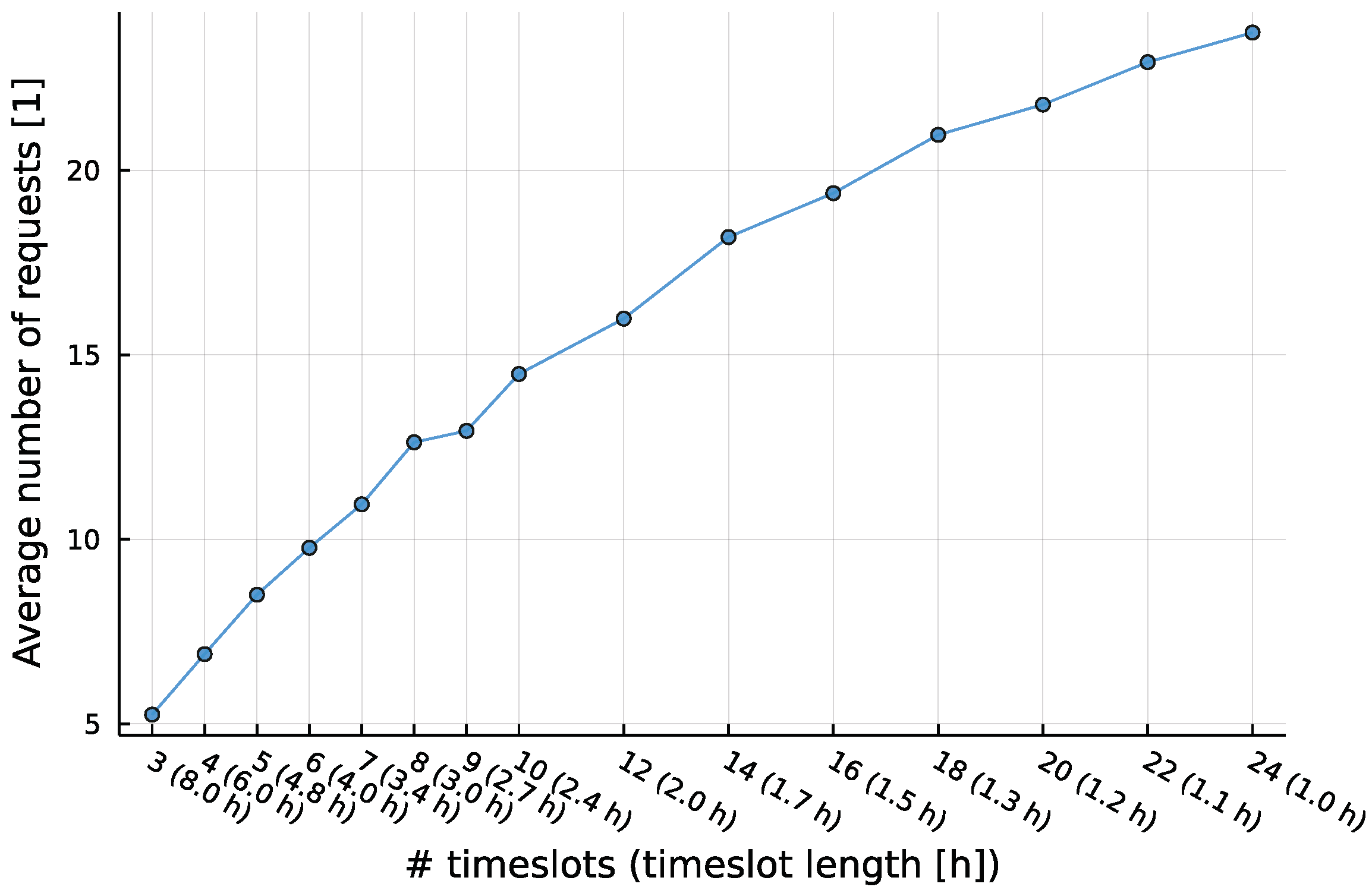
For the first experiment, we generate 15 parametric problem instances with different charging timeslot sizes (between 8 h and 1 h) and a different number of timesteps (each instance having the number of timesteps equal to the number of timeslots times 8). We set the demand scaling parameter, the expected number of requested timeslots, so that the total requested charging duration (The expected total requested charging duration according to the MDP distributions, not the sum of charging duration of all sampled requests) of all charging sessions is $2/3$ of the total charging capacity. The charging location is equipped with three charging points capable of serving three simultaneous charging sessions.

The charging requests are sampled from the discretized distributions described in Section 5.1. Note that this configuration means that the number of requests increases with the number of timeslots and their average duration decreases (see Figure 4). Furthermore, the demand for charging is disproportionately concentrated to the middle of the day (see Figure 3), meaning that this scenario can be considered a high-demand scenario, where it is likely that not all demand can be satisfied with the available capacity.

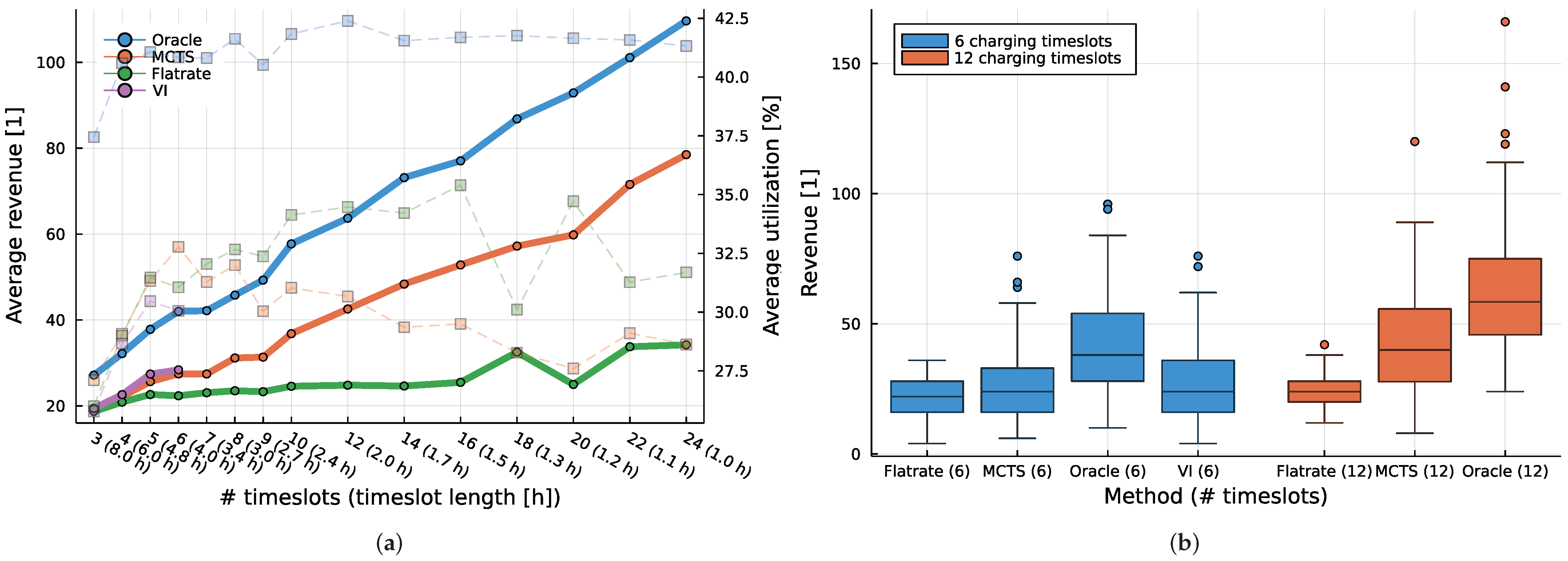
In this scenario, we first optimize for revenue and utilization with each of our methods. For each problem instance, we sample 100 charging request sequences and calculate the revenue and utilization of every method. The averaged results of these experiments when optimizing revenue are given in Figure 5, while the utilization-optimizing results are shown in Figure 6. In both figures, we see that the oracle is indeed the upper bound on the performance of any pricing method due to the availability of perfect information that this method assumes.

In the case of revenue optimization (Figure 5a), the VI baseline, which provides realistic in-expectation optimal pricing solutions, can solve problem instances with up to 6 timeslots. Above 6, we ran out of memory for representing the state-space. The MCTS solution performs well when compared to the VI and manages to outperform the flat rate by a wide margin, shadowing the performance of the oracle baseline. However, when optimizing for revenue, the flat rate generates higher utilization than MCTS.

Notably, in Figure 5a, the revenue of the oracle baseline and MCTS increases with an increasing number of timeslots. This is caused by the fact that we keep the total requested charging duration the same in all problem instances. Increasing the number of timeslots increases the number of individual charging requests. The finer timeslot discretization allows the total expected charging duration to be split up into more differently sized charging sessions. The oracle and MCTS can leverage this larger number of requests to prefer requests from EV users with higher budgets. Since the flat rate can not respond this way, the revenue from the flat rate remains level.

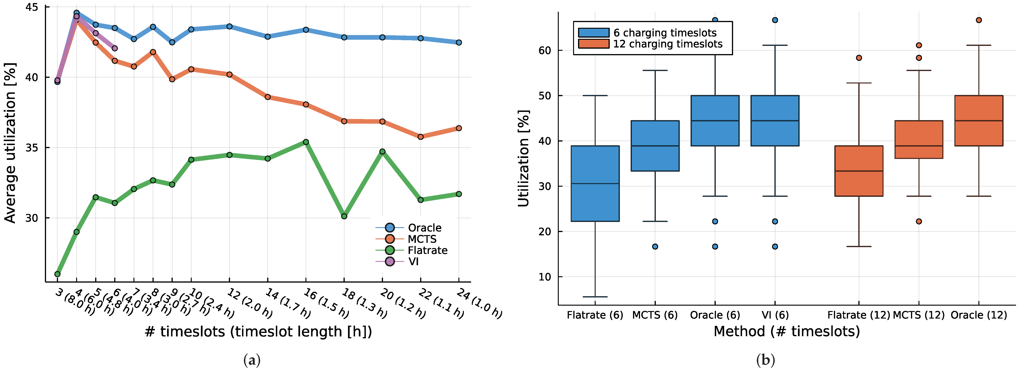
When optimizing utilization (Figure 6a), unlike in the previous case, the dynamic pricing methods can not exploit the high budgets of some EV users to boost performance. However, while both flat-rate and oracle give, for the most part, steady performance, the utilization of MCTS slowly falls as the number of requests and timeslots increases (while still shadowing the VI performance where VI can generate results). Here, the cause is again a larger number of more fine-grained requests. The smaller granularity means there is a greater chance of overlap among the requests. While oracle can readily prevent overlap due to its nature, this is not the case for MCTS. The task becomes increasingly difficult as the number of requests (timeslots) increases. The higher number and shorter duration of charging requests (while the total requested charging duration of all requests is kept constant) provide an opportunity for dynamic pricing to increase revenue through allocating resources to higher-paying EV drivers. We show that MCTS dynamic pricing can leverage this, closely shadowing the optimal VI where the comparison is available. Coincidentally, the introduction of long-distance, very fast EV charging stations such as the Tesla superchargers mean higher number and shorter charging sessions in high-demand locations such as highways. Such locations could be a prime candidate for the dynamic pricing scheme discussed in this paper. On the other hand, more fine-grained demand means more overlapping charging sessions, and MCTS can again improve the performance over the flat rate. However, the performance decreases as the number of requests rises.

5.4.2. Variable-Demand Experiment

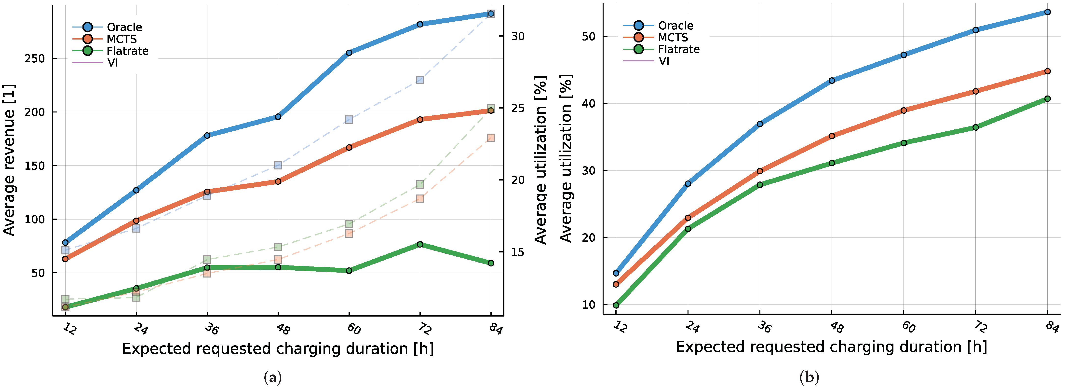
In the second experiment, we fix the number of timeslots to 48, resulting in each timeslot lasting 30 min. Then we vary the total requested charging duration from 12 h to 84 between the different problem instances. The lower limit corresponds to a low demand situation, with the expected number of requests being only $17\%$ of the total CS capacity of 72 charging hours, and the upper limit representing a very high demand scenario where all of the requested capacity can not be possibly satisfied.

Again, we sample 100 charging request sequences from each problem instance and average the results. These results when optimizing for revenue are shown in Figure 7a, while the optimization for utilization is in Figure 7b.

MCTS outperforms flat-rate in both experiments, with increasing gains as demand increases in both experiments. When optimizing for revenue, the revenue of MCTS is much greater than that of flat-rate, while the utilization remains comparable (Figure 7a).

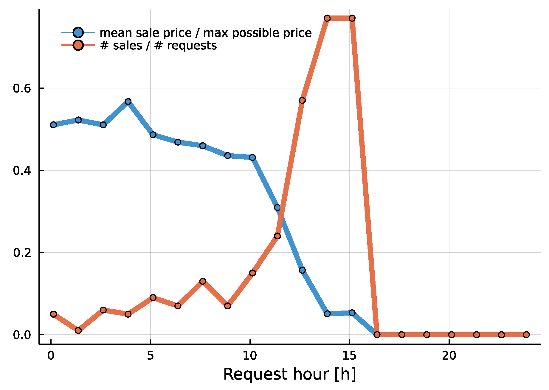
Using the same problem instance with total expected demand of 48 charging hours, we also illustrate the pricing response of MCTS to different states in Figure 8. The figure demonstrates the changes in price offered by the MCTS for a one hour long charging session at 16:00. Initially, the price is quite steep, but as the start of the charging session approaches, the price is reduced to almost, finally reaching zero at the start of the charging session.

Overall, the MCTS improves both revenue and utilization as demand increases, shadowing the performance of the oracle baseline. Regarding the runtime of the MCTS pricing, it takes at most 9 ms to generate the estimate of the best action in any state of any problem instance discussed in this work (running on a single core of an Intel(R) Core(TM) i7-3930K CPU @ 3.20 GHz).

6. Conclusions and Future Work

Dynamic pricing schemes have been in the market for more than two decades. Due to their success in different application domains such as booking airline and hotel tickets, the concept was also adopted in the field of energy systems. It is a promising method of demand-side management, where grid operators use it to change the demand of the end-users during shortage periods.

Recently, dynamic pricing was also applied to the charging of electric vehicles (EVs). In this paper, we studied dynamic pricing in the context of EV charging to maximize either (1) the revenue of the CS operator or (2) the overall utilization of the available capacity. Using Markov Decision Process methodology, we formulated the aforementioned problem and proposed a heuristic based on Monte Carlo Tree Search (MCTS). The successful application of MCTS to the dynamic pricing of EV charging problem is a novel contribution of this paper. We carried out the experiments using a real-world dataset from a German CS operator and compared flat-rate, value iteration, and oracle scenarios with our proposed MCTS-based pricing.

The results of our first experiment (Figure 5 and Figure 6) have shown that the proposed MCTS method achieved at least $93.6\%$ of revenue of the optimal pricing policy provided by the VI, and it did so without significantly increasing the variance of the results. Additionally, we have shown MCTS scaled to up to ten orders of magnitude larger problem instances than VI (in terms of the state space size).

Furthermore, the experiments with changing demand levels (Figure 7) have shown that our MCTS method achieves higher revenue for CS operators than the one realized by the flat-rate scheme, with up to $3.5$ times higher revenues. However, our results indicate that such revenue-maximizing optimization leads up to $8\%$ lower utilization of the charging station. Nevertheless, when optimizing utilization, MCTS could deliver up to $32\%$ higher utilization than the flat rate.

Since MDPs allow for a combination of different criteria in the reward function, one possible direction for future work would be an investigation of other different optimization goals and their combinations, for example, one that would increase revenue without significantly reducing utilization. Other possible directions of future work include an extension to multiple, geographically separate charging locations, or improvements to the user model so that users can attempt to adjust their requests in order to satisfy their charging needs.

The existing model MDP model also has room for improvement. The state-space could be reduced by changing the dimension of the capacity and product vectors as timeslots become unavailable. In the MCTS method, we can likely improve the performance by incorporating more domain knowledge, such as domain informed rollout policies. Additionally, in principle, the MCTS method could be modified to work with continuous timesteps and actions. In the evaluation, we could get closer to a realistic scenario by incorporating the distributions of real user budgets and real lead times from other domains into the evaluation.