
Use of Machine Learning for Leak Detection and Localization in Water Distribution Systems


Abstract
:1. Introduction
2. Materials and Methods
2.1. Research Methodology
2.2. Data Generation
2.3. Use of Machine Learning Methods
2.4. Input and Output Parameters
3. Results
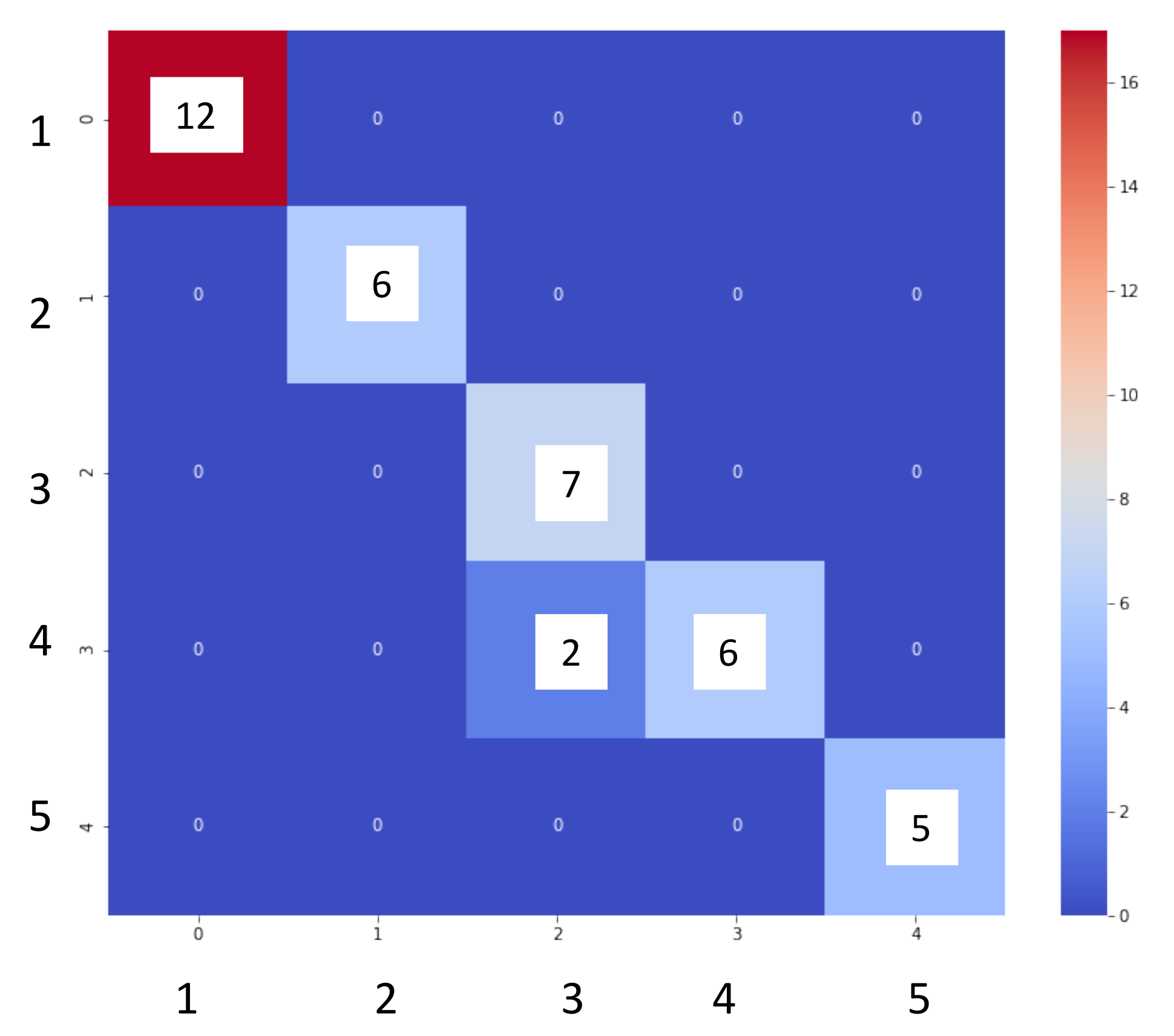
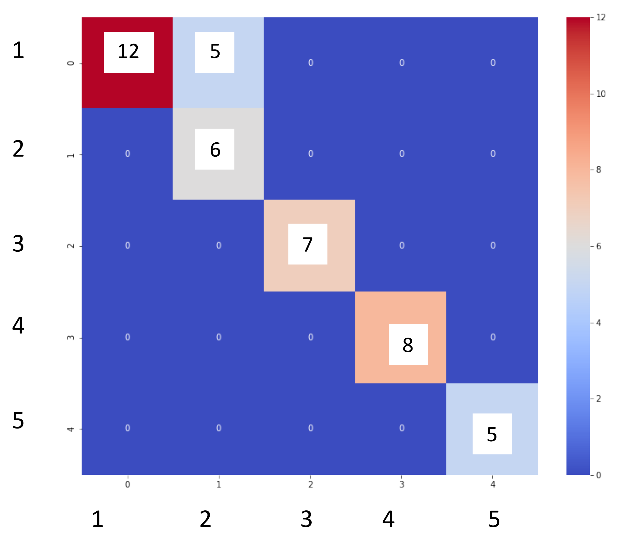
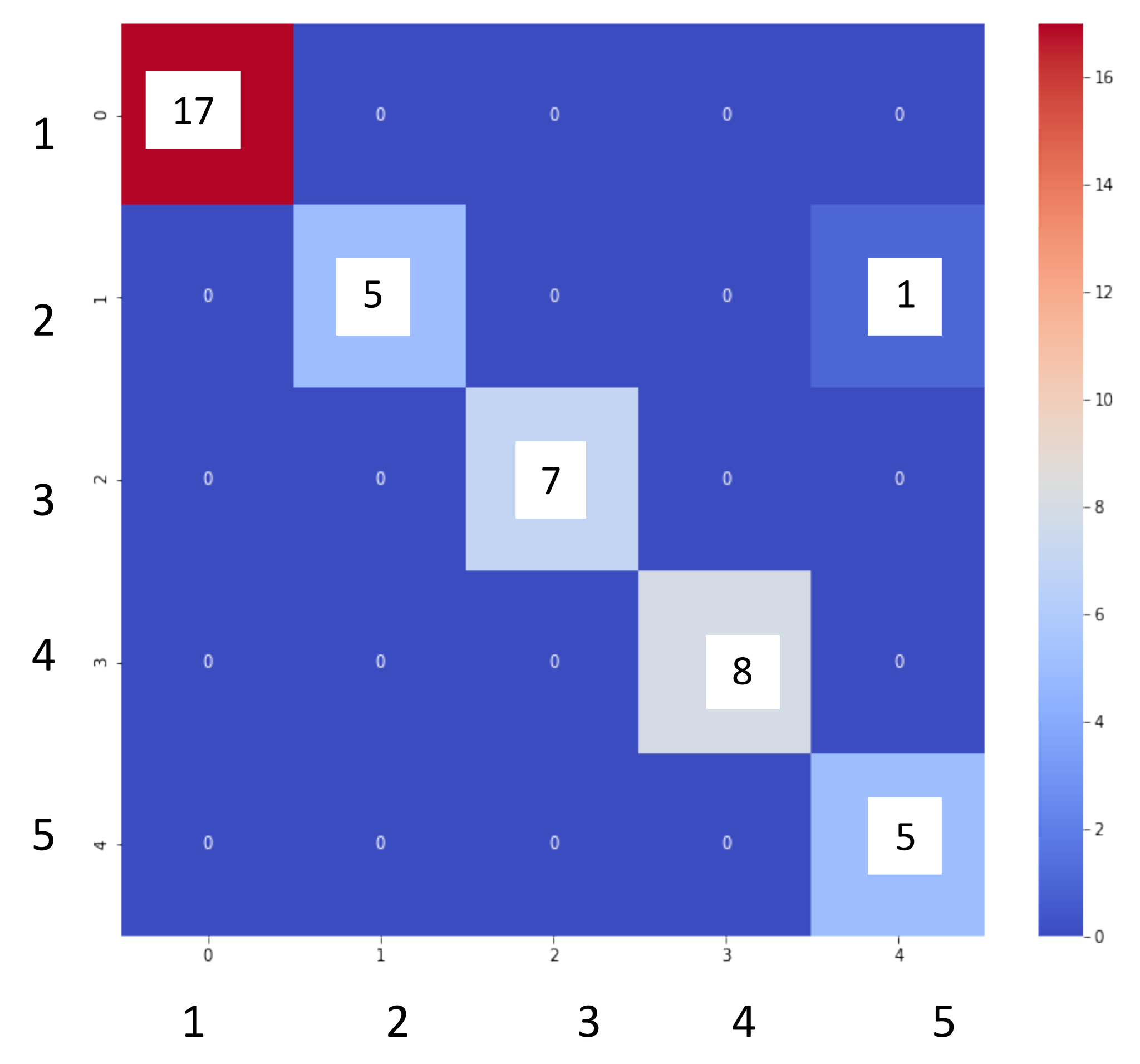
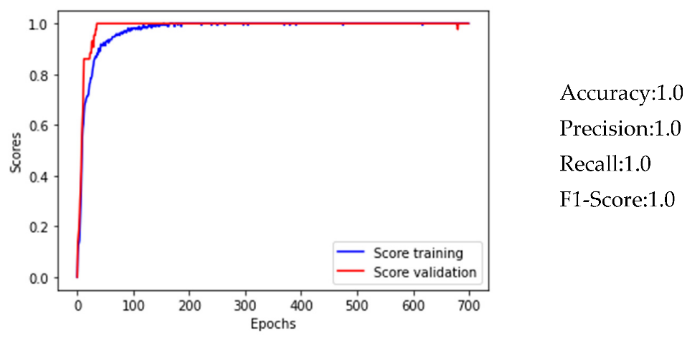
3.1. Supervised Methods
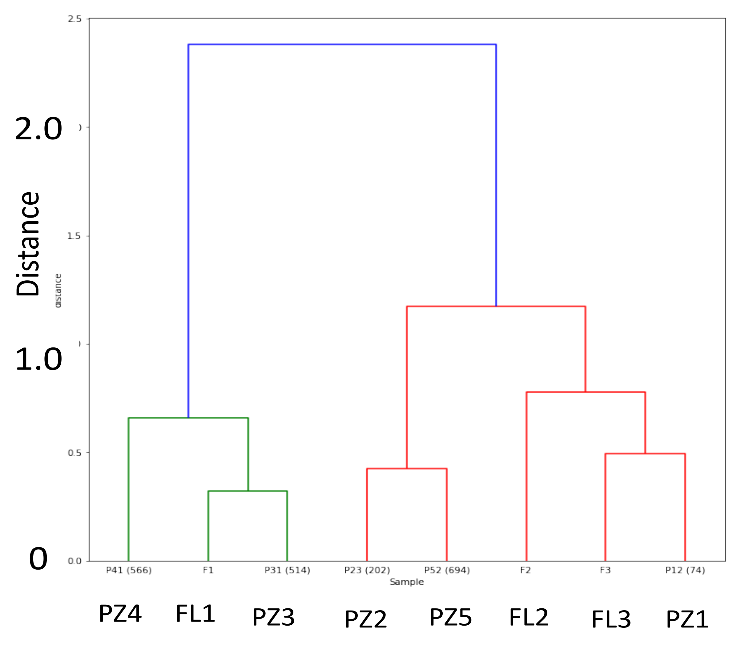
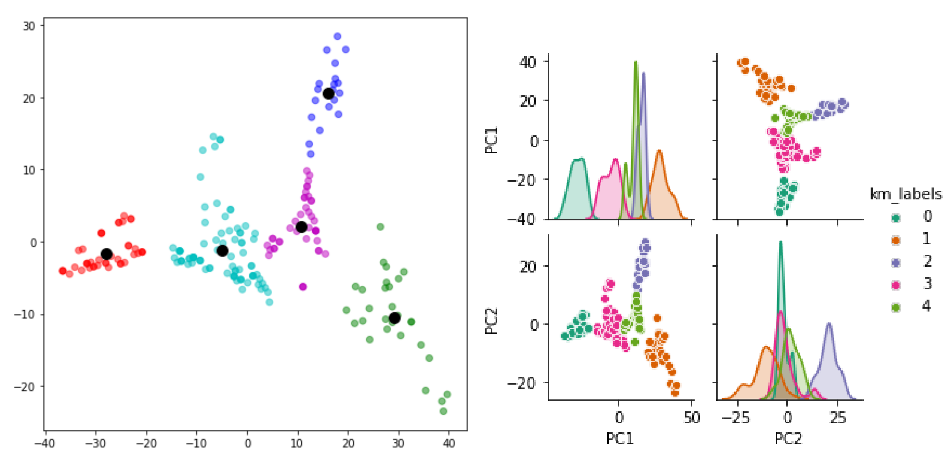
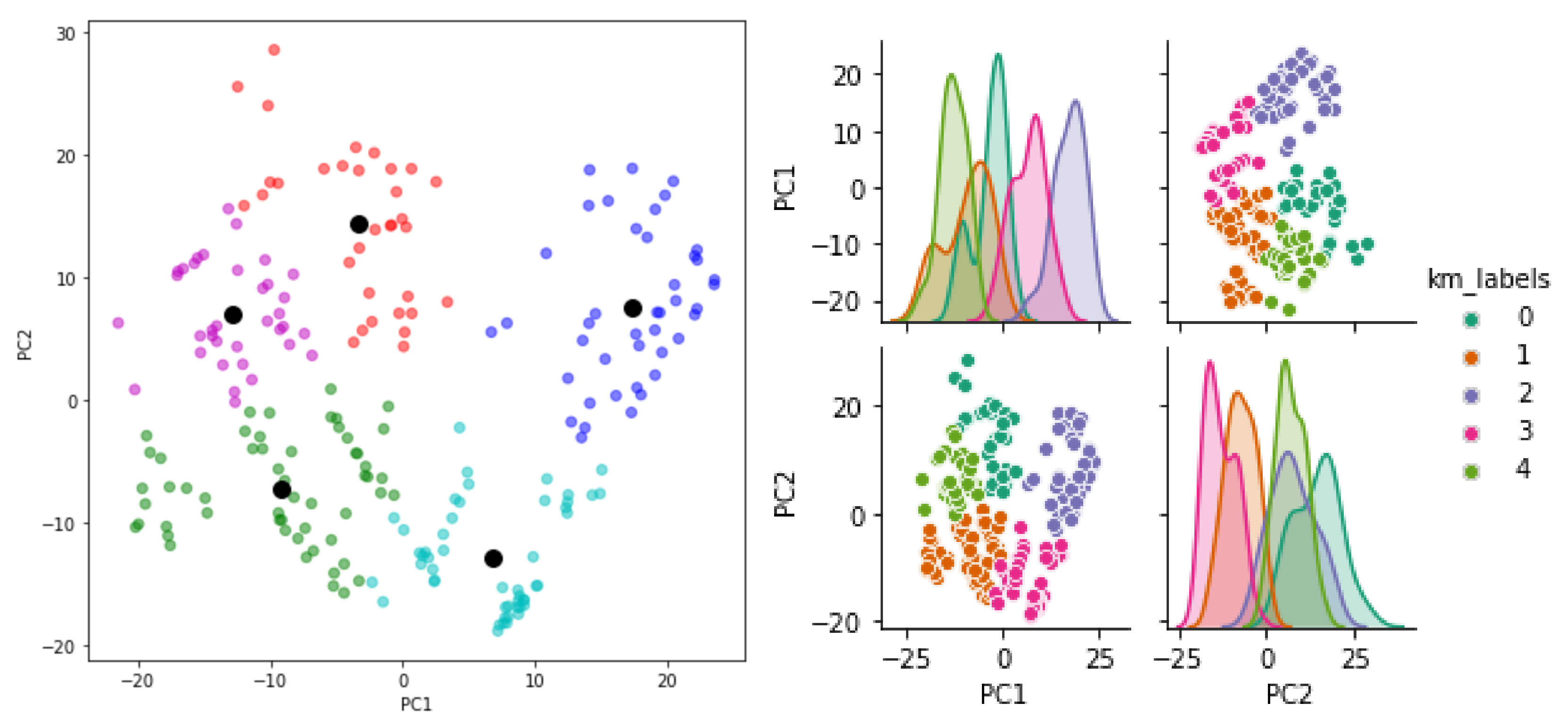
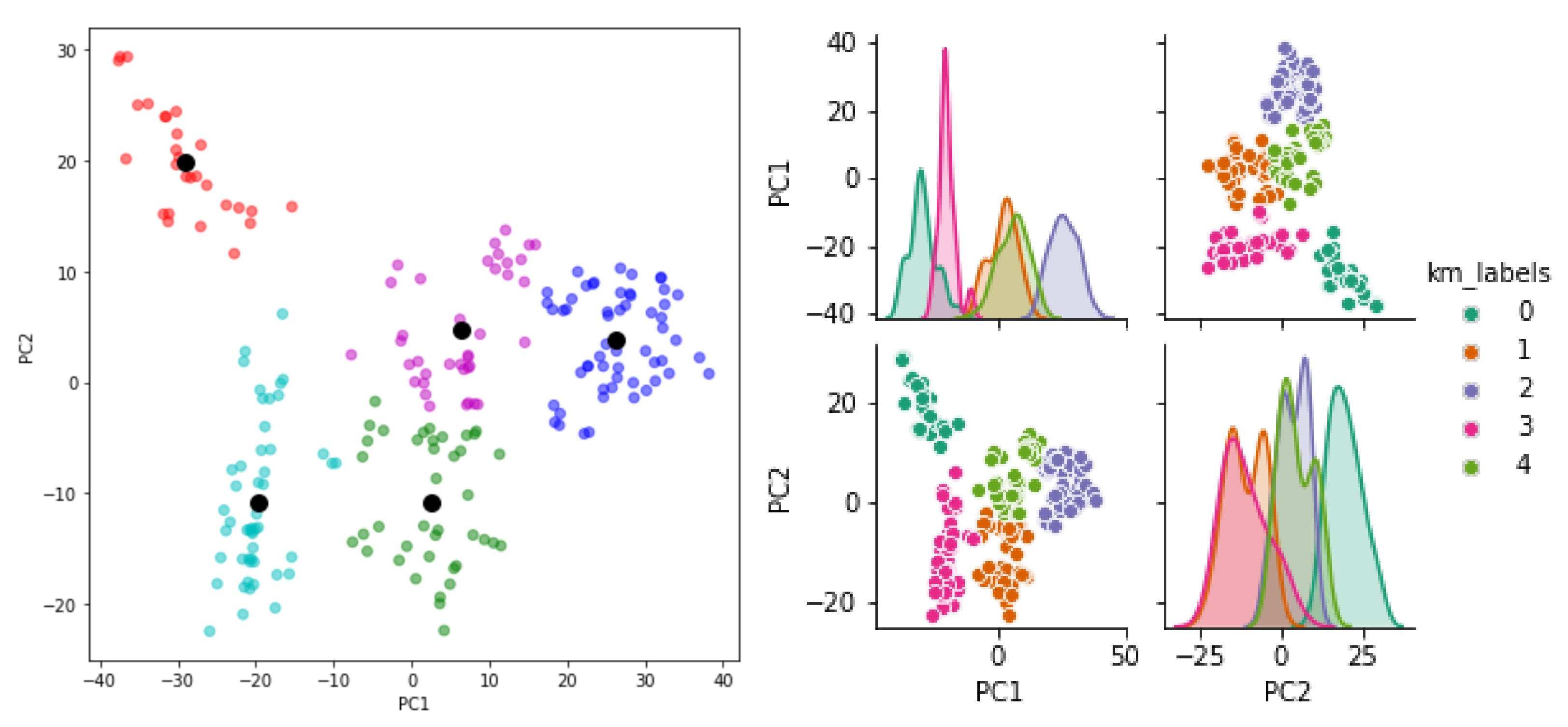
3.2. Unsupervised Methods
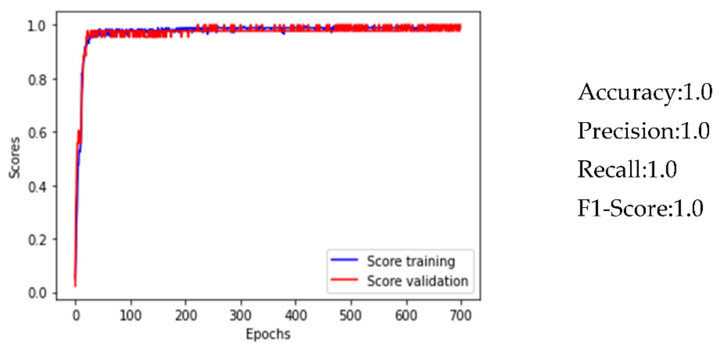
3.3. Artificial Neural Network
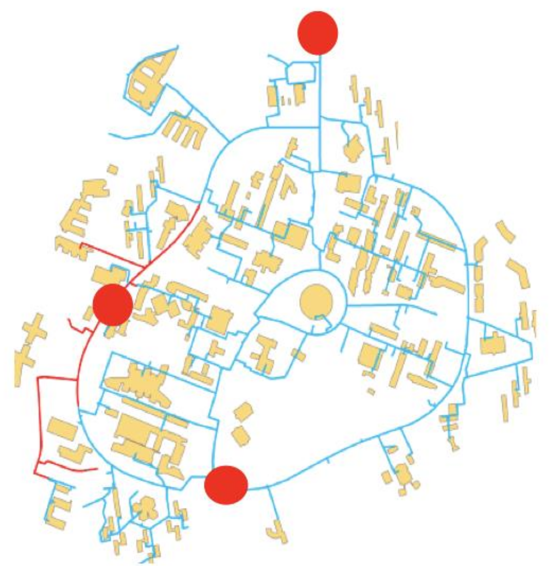
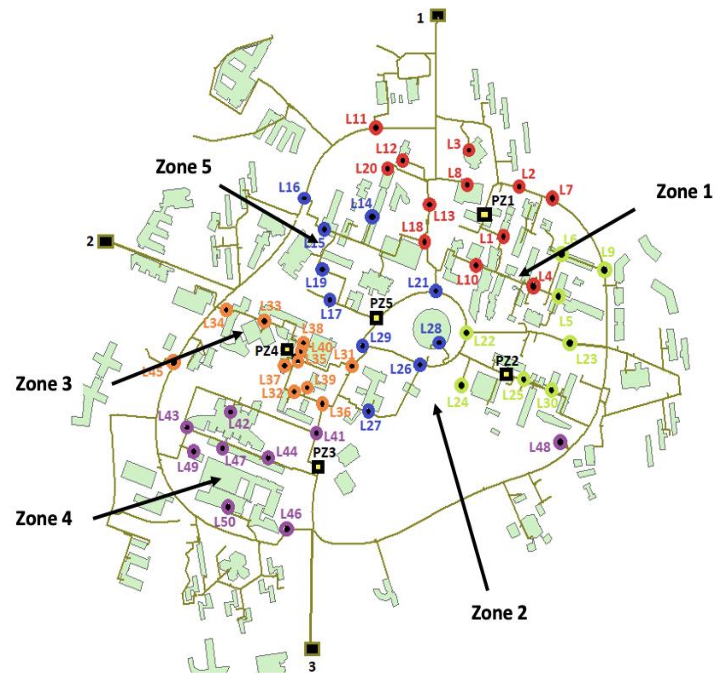
3.4. Analysis of the Water Leak in the Scientific Campus of Lille University
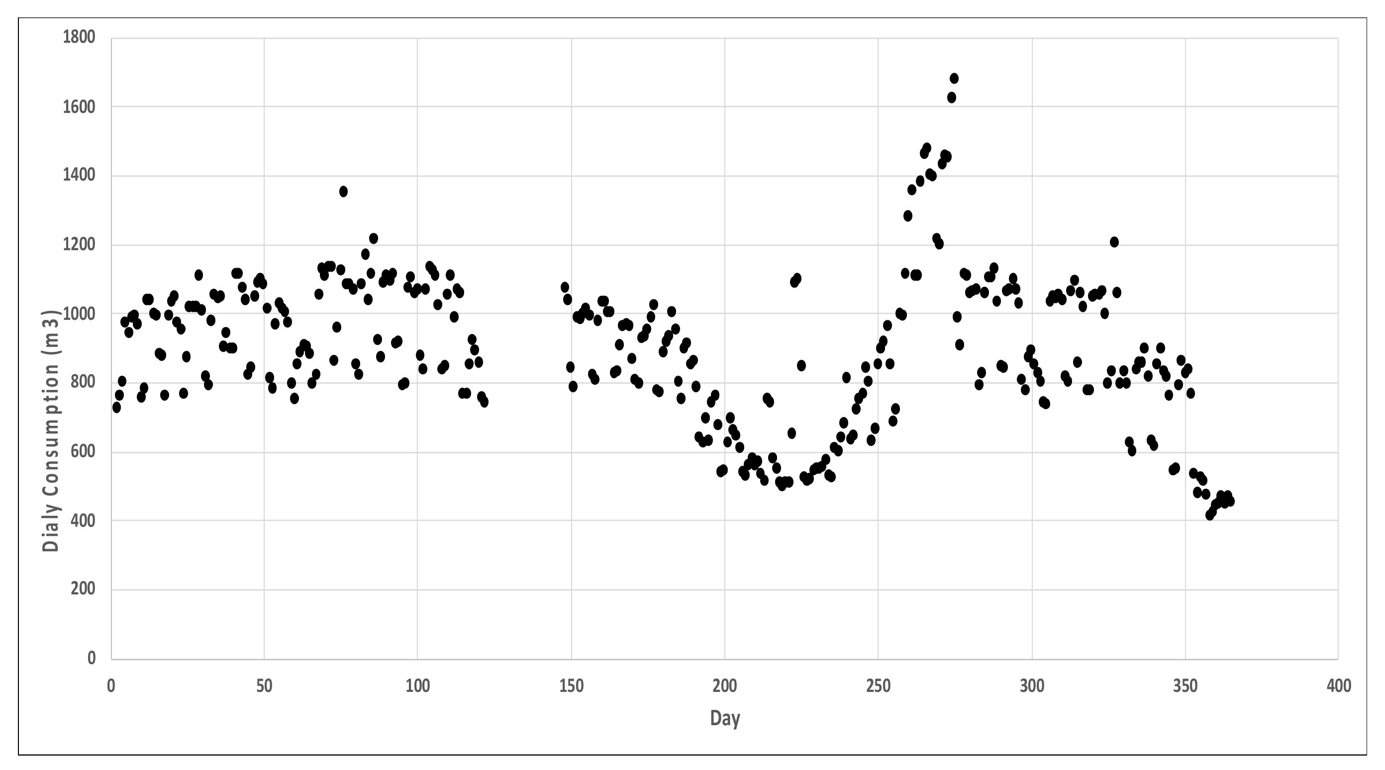
3.5. Analysis of the Daily Water Consumption (Qd)
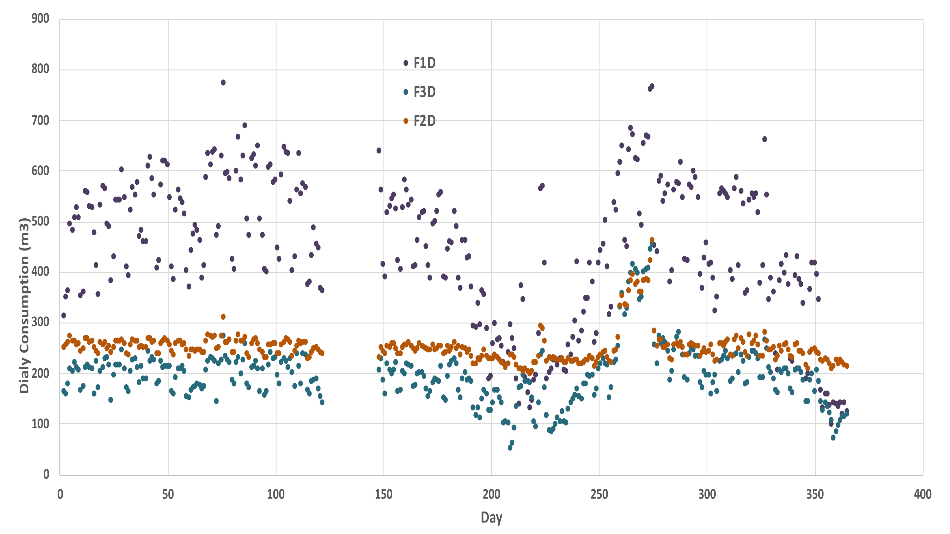
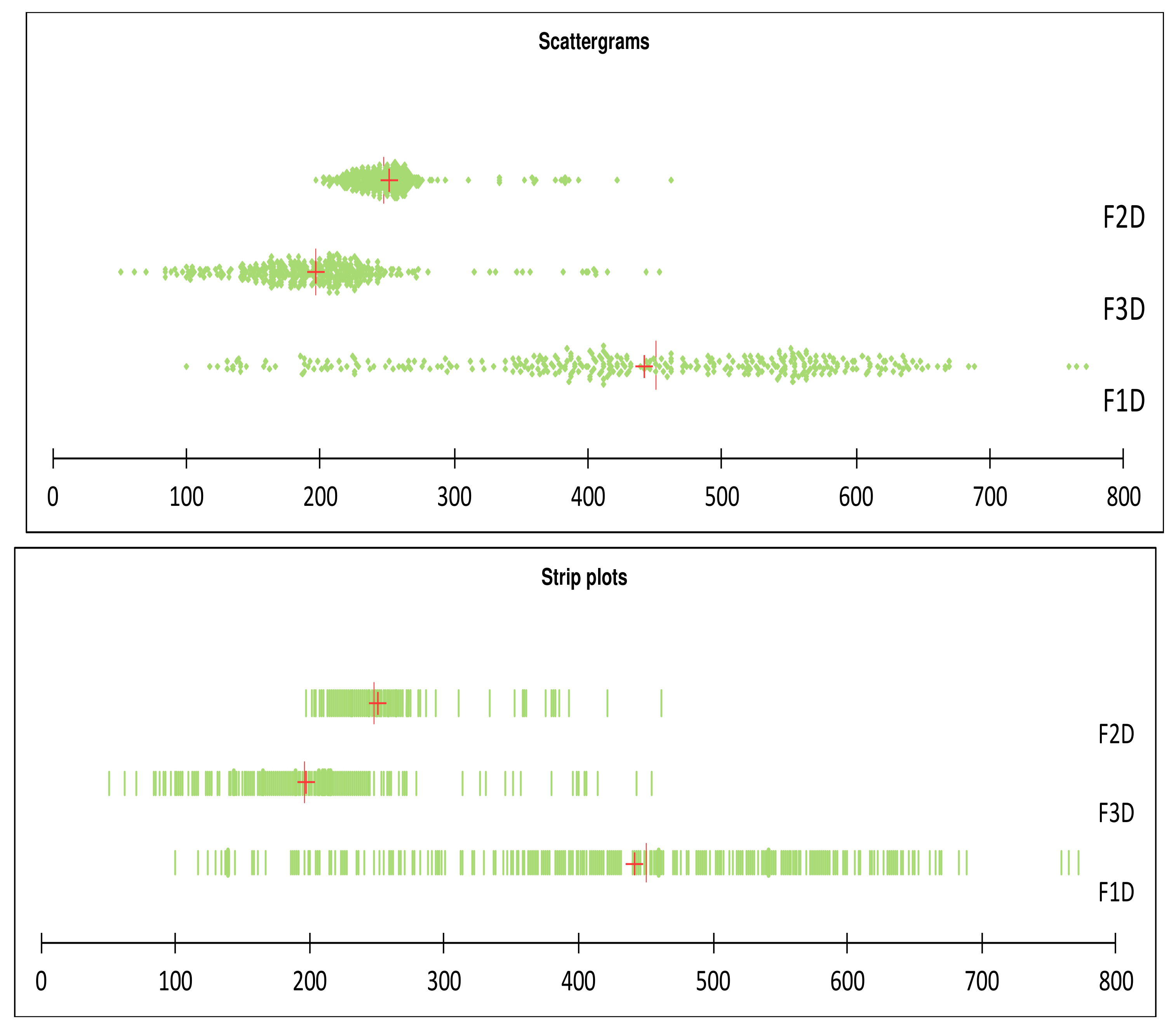
3.6. Leakage Analysis
3.7. Leakage Localization
4. Discussion
- Three supervised methods: logistic regression, decision tree, and random forest;
- Two unsupervised methods: The hierarchical classification method and a combination of the PCA and K-means classification method;
- The ANN
- Excellent performance of the supervised methods in the localization of leaks in the water network. Both the logistic regression and the random forest predicted the position of the leak with an accuracy = 1.0. In contrast, the decision tree predicted leaks with an accuracy = 0.98 with pressure and flow data;
- Excellent performances by the ANN for the localization of water leaks in the water network (accuracy = 1.0);
- Some difficulties in exploiting the clustering capacity of the unsupervised methods in the leak localization because of overlapping clusters.
5. Conclusions
Author Contributions
Funding
Institutional Review Board Statement
Informed Consent Statement
Data Availability Statement
Conflicts of Interest
References
- Kingdom, B.; Liemberger, R.; Marin, P. The Challenge of Reducing Non-Revenue (NRW) Water in Developing Countries. How the Private Sector Can Help: A Look at Performance-Based Service Contracting; Water Supply and Sanitation (WSS) Sector Board Discussion Paper N. 8; The World Bank: Washington, DC, USA, 2006. [Google Scholar]
- Thornton, J.; Sturm, R.; Kunkel, G. Water Loss Control, 2nd ed.; McGraw Hill: New York, NY, USA, 2008; ISBN 9780071499187. [Google Scholar]
- Renzetti, S.; Dupont, D. Buried Treasure: The Economics of Leak Detection and Water Loss Prevention in Ontario. Environmental Sustainability Research Centre (ESRC) Working Paper Series. 2013. Available online: http://hdl.handle.net/10464/4279 (accessed on 30 June 2021).
- Kanakoudis, V.K. A troubleshooting manual for handling operational problems in water pipe networks. Water Supply Res. Technol.-AQUA 2004, 53, 109–124. [Google Scholar] [CrossRef]
- Hunaidi, O.; Wang, A.; Bracken, M.; Gambino, T.; Fricke, C. Acoustic methods for locating leaks in municipal water pipe networks. In Proceedings of the International Conference on Water Demand Management, Dead Sea, Jordan, 30 May–3 June 2004; pp. 1–14. [Google Scholar]
- Adegboye, M.A.; Fung, W.-K.; Karnik, A. Recent Advances in Pipeline Monitoring and Oil Leakage Detection Technologies: Principles and Approaches. Sensors 2019, 19, 2548. [Google Scholar] [CrossRef] [Green Version]
- Fahmy, M.; Moselhi, O. Detecting and locating leaks in underground water mains using thermography. In Proceedings of the 26th International Symposium on Automation and Robotic in Construction (ISARC), Austin, TX, USA, 24–27 June 2009; pp. 61–67. [Google Scholar]
- Ayala–Cabrera, D.; Herrera, M.; Izquierdo, J.; Ocaña–Levario, S.; Pérez–García, R. GPR-Based Water Leak Models in Water Distribution Systems. Sensors 2013, 13, 15912–15936. [Google Scholar] [CrossRef]
- Noran, P.; Obenauf, P. Asset Management of a Failing 36" Ductile Iron Sewage Force Main. In Pipelines 2010; American Society of Civil Engineers: Reston, WV, USA, 2010; pp. 566–576. [Google Scholar] [CrossRef]
- Zhang, X. Statistical leak detection in gas and liquid pipelines. Pipes Pipelines Int. 1993, 38, 20–26. [Google Scholar]
- Buchberger, S.G.; Nadimpalli, G. Leak Estimation in Water Distribution Systems by Statistical Analysis of Flow Readings. J. Water Resour. Plan. Manag. 2004, 130, 321–329. [Google Scholar] [CrossRef]
- Lambert, A. International report: Water losses management and techniques. Water Sci. Technol. Water Supply 2002, 2, 1–20. [Google Scholar] [CrossRef] [Green Version]
- Billmann, L.; Isermann, R. Leak detection methods for pipelines. Automatica 1987, 23, 381–385. [Google Scholar] [CrossRef]
- Silva, R.; Buiatti, C.; Cruz, S.; Pereira, J. Pressure wave behaviour and leak detection in pipelines. Comput. Chem. Eng. 1996, 20, S491–S496. [Google Scholar] [CrossRef]
- Caputo, A.C.; Pelagagge, P.M. Using Neural Networks to Monitor Piping Systems. Process Saf. Prog. 2003, 22, 119–127. [Google Scholar] [CrossRef]
- Salam, A.E.U.; Tola, M.; Selintung, M.; Maricar, F. On-line monitoring system of water leakage detection in pipe networks with artificial intelligence. ARPN J. Eng. Appl. Sci. 2014, 9, 1817–1822. [Google Scholar]
- Mounce Stephen, R.; Mounce, R.B.; Boxall, J.B. Novelty detection for time series data analysis in water distribution systems using support vector machines. J. Hydroinformatics 2011, 13, 672–686. [Google Scholar] [CrossRef]
- Rojek, I.; Studzinski, J. Detection and localization of water leaks in water nets supported by an ICT system with artificial intelligence methods as a way forward for smart cities. Sustainability 2019, 11, 518. [Google Scholar] [CrossRef] [Green Version]
- Zhang, Q.; Wu, Z.Y.; Zhao, M.; Qi, J.; Huang, Y.; Zhao, H. Leakage Zone Identification in Large-Scale Water Distribution Systems Using Multiclass Support Vector Machines. J. Water Resour. Plan. Manag. 2016, 142, 4016042. [Google Scholar] [CrossRef]
- Chan, T.K.; Chin, C.S.; Zhong, X. Review of Current Technologies and Proposed Intelligent Methodologies for Water Distributed Network Leakage Detection. IEEE Access 2018, 6, 78846–78867. [Google Scholar] [CrossRef]
- Soldevila, A.; Blesa, J.; Tornil-Sin, S.; Duviella, E.; Fernandez-Canti, R.M.; Puig, V. Leak localization in water distribution networks using a mixed model-based/data-driven approach. Control Eng. Pract. 2016, 55, 162–173. [Google Scholar] [CrossRef] [Green Version]
- Ciupke, K. Leak Detection Using Regression Trees. In Advances in Technical Diagnostics. ICDT 2016. Applied Condition Monitoring; Timofiejczuk, A., Łazarz, B., Chaari, F., Burdzik, R., Eds.; Springer: Cham, Switzerland, 2018; Volume 10. [Google Scholar] [CrossRef]
- van der Walt, J.C.; Heyns, P.S.; Wilke, D.N. Pipe network leak detection: Comparison between statistical and machine learning techniques. Urban Water J. 2018, 15, 953–960. [Google Scholar] [CrossRef]
- Shahrour, I.; Abbas, O.; Abdallah, A.; AbouRjeily, Y.; Afaneh, A.; Aljer, A.; Ayari, B.; Farrah, E.; Sakr, D.; Al Masri, F. Lessons from a Large-Scale Demonstrator of the Smart and Sustainable City BT—Happy City—How to Plan and Create the Best Livable Area for the People; Brdulak, A., Brdulak, H., Eds.; Springer International Publishing: Berlin/Heidelberg, Germany, 2017; pp. 193–206. [Google Scholar] [CrossRef]
- Farah, E.; Shahrour, I. Leakage Detection Using Smart Water System: Combination of Water Balance and Automated Minimum Night Flow. Water Resour. Manag. 2017, 31, 4821–4833. [Google Scholar] [CrossRef]
- Farah, E.; Abdallah, A.; Shahrour, I. SunRise: Large scale demonstrator of the smart water system. Int. J. Sustain. Dev. Plan. 2017, 12, 112–121. [Google Scholar] [CrossRef]
- Harrell, F.E. Regression Modeling Strategies; Springer: Berlin/Heidelberg, Germany, 2001; ISBN 0-387-95232-2. [Google Scholar]
- Breiman, L.; Friedman, J.H.; Olshen, R.A.; Stone, C.J. Classification and Regression Trees; Wadsworth, Inc.: Belmont, CA, USA, 1984. [Google Scholar]
- Lin, N.; Noe, D.; He, X. Tree-based methods and their applications In Springer Handbook of Engineering Statistics; Pham, H., Ed.; Springer: London, UK, 2006; pp. 551–570. [Google Scholar]
- Prinzie, A.; Van den Poel, D. Random Forests for multiclass classification: Random MultiNomial Logit. Expert Syst. Appl. 2008, 34, 1721–1732. [Google Scholar] [CrossRef]
- Breiman, L. Random Forests. Mach. Learn. 2001, 45, 5–32. [Google Scholar] [CrossRef] [Green Version]
- Ward, J.H., Jr. Hierarchical Grouping to Optimize an Objective Function. J. Am. Stat. Assoc. 1963, 58, 236–244. [Google Scholar] [CrossRef]
- Mohamad Asri, M.N.; Mat Desa, W.N.S.; Ismail, D. Combined Principal Component Analysis (PCA) and Hierarchical Cluster Analysis (HCA): An efficient chemometric approach in aged gel inks discrimination. Aust. J. Forensic Sci. 2020, 52, 38–59. [Google Scholar] [CrossRef]
- Hartigan, J.A.; Wong, M.A. Algorithm AS 136: A K-Means Clustering Algorithm. J. R. Stat. Soc. Ser. C 1979, 28, 100–108. [Google Scholar] [CrossRef]
- Dave, V.S.; Dutta, K. Neural network-based models for software effort estimation: A review. Artif. Intell. Rev. 2014, 42, 295–307. [Google Scholar] [CrossRef]


| Actual | Prediction | ||
| Positive | Negative | ||
| Positive | True Positive | False Negative | |
| Negative | False Positive | True Negative | |
| Zone | Position of Water Leak |
|---|---|
| 1 (62 leak scenarios) | L1, L2, L4, L7, L8, L10, L13, L18, L20 L10 + L11; L10 + L12; L10 + L13; L10 + L18; L10 + L2; L10 + L20; L10 + L3; L10 + L4; L10 + L7; L10 + L8; L11 + L12; L11 + L13; L11 + L18; L11 + L2; L11 + L20; L11 + L3: L11 + L4; L11 + L7; L11 + L8; L12 + L13; L12 + L18; L12 + L2; L12 + L20; L12 + L4; L12 + L7; L12 + L8; L13 + L18; L13 + L2; L13 + L20; L13 + L3; L13 + L4; L13 + L7; L13 + L8; L18 + L2; L18 + L20; L18 + L3; L18 + L4; L18 + L7; L18 + L8; L2 + L20; L2 + L4; L2 + L7; L2+ L8; L1 + L10; L1 + L11; L1 + L12; L1 + L13; L1 + L18; L1 + L2; L1 + L20; L1 + L3; L1 + L4; L1 + L7; L1 + L8 |
| 2 (35 leak scenarios) | L5, L6, L9, L22, L23, L24, L25, L30 L23 + L22; L24 + L22; L24 + L23; L25 + L22; L25 + L23; L25 + L24; L30 + L22; L30 + L23; L30 + L24; L30 + L25; L5 + L22; L5 + L23; L5 + L24; L5 + L25; L5 + L30; L6 + L22; L6 + L24; L6 + L25; L6 + L30; L6 + L5; L9 + L22; L9 + L23; L9 + L24; L9 + L25; L9 + L30; L9 + L5; L9 + L6: |
| 3 (30 leak scenarios) | L41, L42, L43, L44, L46, L47, L48, L49, L50 L41 + L44; L41 + L46; L41 + L47; L41 + L48; L41 + L50; L42 + L44; L42 + L46; L42 + L47; L42 + L48; L42 + L50; L43 + L44; L43 + L46; L43 + L47; L43 + L48; L43 + L50; L44 + L46; L44 + L47; L44 + L48; L44 + L50; L46 + L47; L47 + L48; L47 + L50; L48 + L49; L50 + L49 |
| 4 (47 leak scenarios) | L31, L32, L33, L34, L35, L36, L37, L38, L39, L40, L45 L31 + L36; L31 + L37; L31 + L38; L31 + L39; L31 + L45; L32 + L36; L32 + L37; L32 + L38; L32 + L39; L32 + L45; L33 + L36; L33 + L37; L33 + L38; L33 + L39; L33 + L45; L34 + L36; L34 + L37; L34 + L38; L34 + L39; L34 + L45; L35 + L36; L35 + L37; L35 + L38; L35 + L39; L35 + L45; L36 + L37; L36 + L38; L36 + L39L36 + L45;L37 + L38; L37 + L39; L37 + L45; L38 + L39; L38 + L45; L39 + L45; L40 + L45 |
| 5 (41 leak scenarios) | L14, L16, L17, L19, L21, L26, L27, L28, L29 L14 + L21; L14 + L26; L14 + L27; L14 + L28; L14 + L29; L15 + L21; L15 + L26; L15 + L27; L15 + L28; L15 + L29; L16 + L21; L16 + L26; L16 + L27; L16 + L28; L16 + L29; L17 + L21; L17 + L26; L17 + L27; L17 + L28; L17 + L29; L19 + L21; L19 + L26; L19 + L27; L19 + L28; L19 + L29; L21 + L26; L21 + L27; L21 + L28; L21 + L29;L26 + L27; L26 + L28; L26 + L29; L27 + L28; L27 + L29; L28 + L29 |
| Zone | 1 | 2 | 3 | 4 | 5 |
|---|---|---|---|---|---|
| Pressure node | PZ1 | PZ2 | PZ3 | PZ4 | PZ5 |
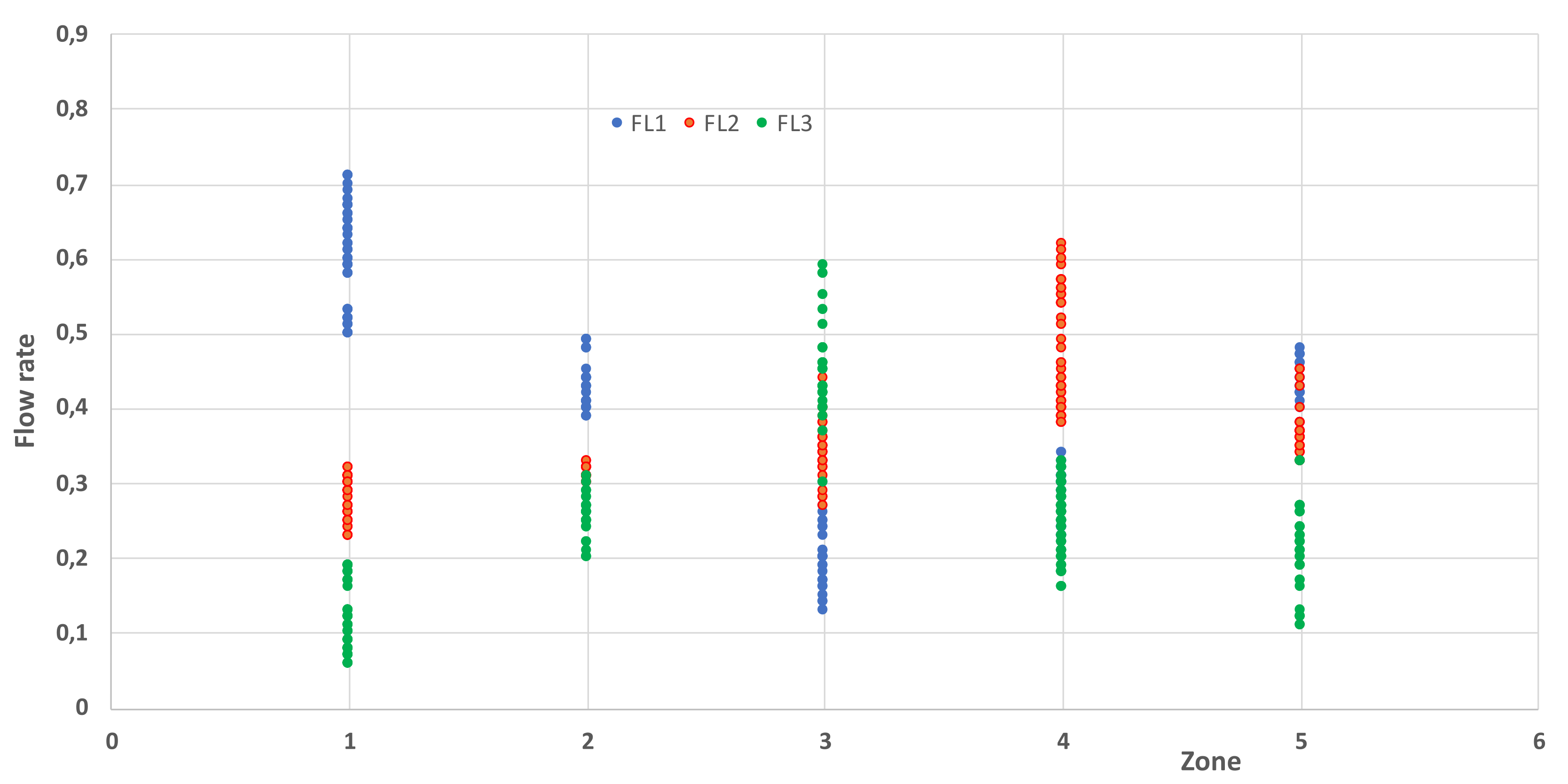
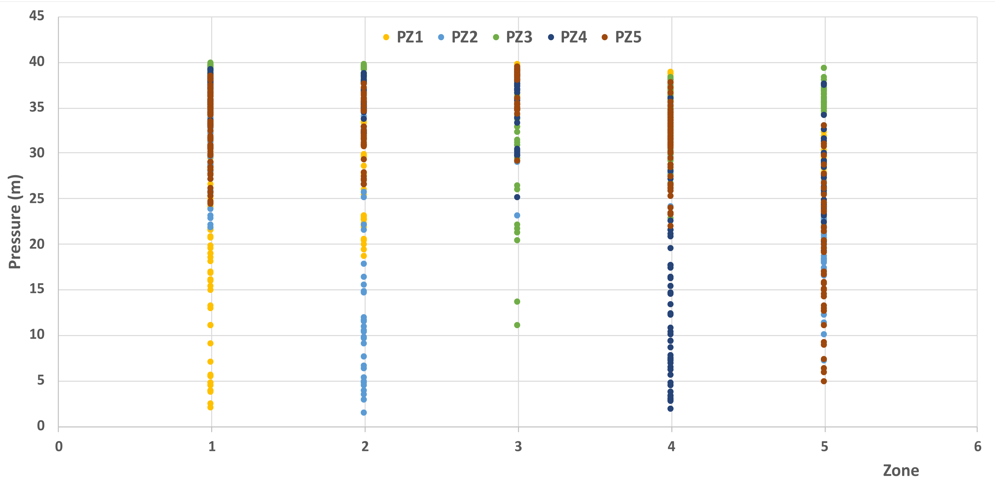
| Minimum | Maximum | Average | Standard Deviation | |
|---|---|---|---|---|
| FL1 (%) | 0.13 | 0.71 | 0.4 | 0.15 |
| FL2 (%) | 0.23 | 0.62 | 0.35 | 0.82 |
| FL3 (%) | 0.60 | 0.59 | 0.23 | 0.11 |
| PZ1 (m) | 2.0 | 39.7 | 28.4 | 9.4 |
| PZ2 (m) | 1.4 | 39.4 | 27.4 | 9.3 |
| PZ3 (m) | 11.0 | 39.8 | 35.6 | 4.5 |
| PZ4 (m) | 1.8 | 39.2 | 29.2 | 10.2 |
| PZ5 (m) | 4.9 | 39.4 | 30.0 | 7.4 |
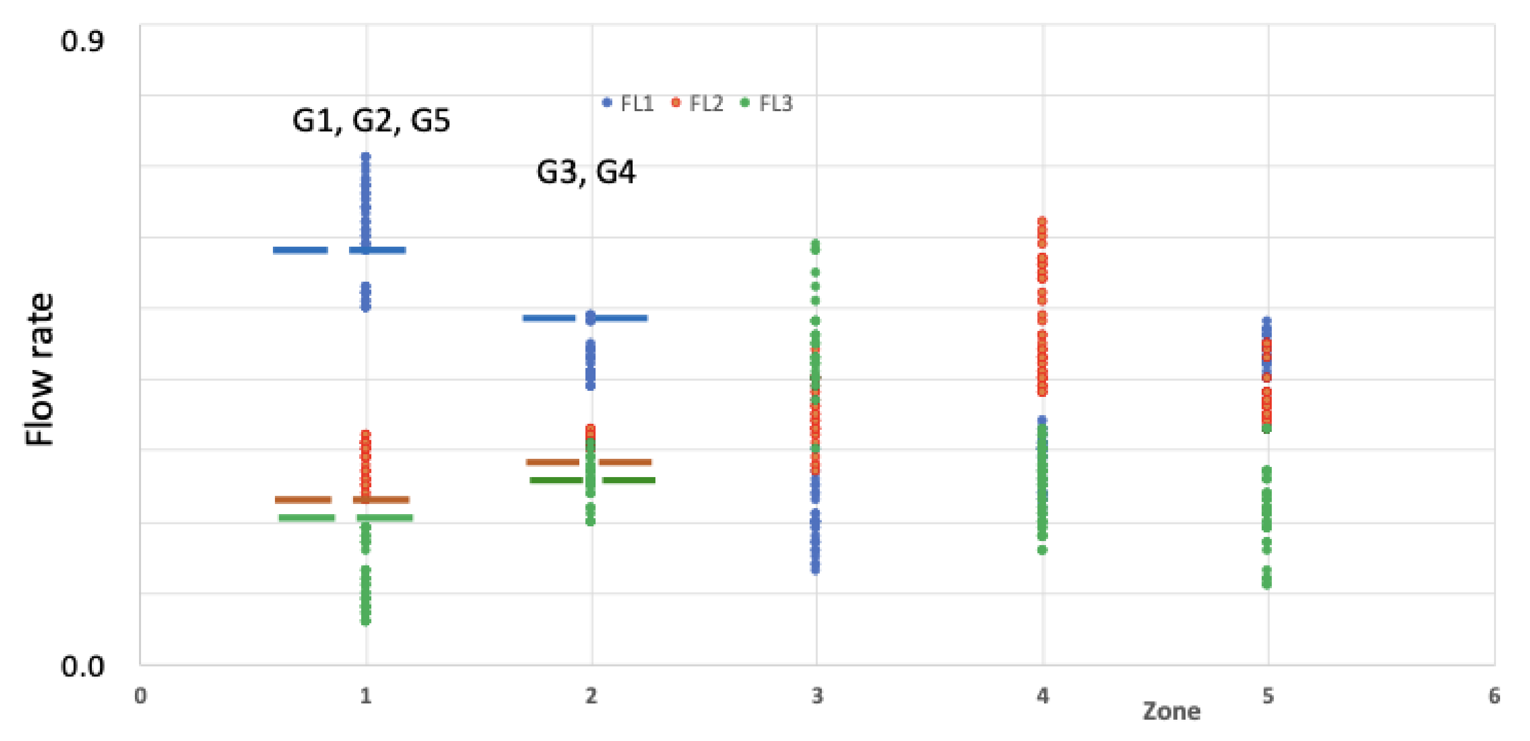
| Leak Zone | FL1 | FL2 | FL3 |
|---|---|---|---|
| 1 | Strong | Medium | Low |
| 2 | Medium | Medium | Low to medium |
| 3 | Low | Medium | Strong |
| 4 | Low | Strong | Low to medium |
| 5 | Medium | Medium | Low to medium |
| Method | Accuracy | Precision | Recall | F1-Score |
|---|---|---|---|---|
| Logistic Regression | 1.0 | 1.0 | 1.0 | 1.0 |
| Decision Tree | 0.95 | 0.96 | 0.95 | 0.95 |
| Random Forest | 1.0 | 1.0 | 1.0 | 1.0 |
| Method | Accuracy | Precision | Recall | F1-Score |
|---|---|---|---|---|
| Logistic Regression | 1.0 | 1.0 | 1.0 | 1.0 |
| Decision Tree | 0.88 | 0.91 | 0.94 | 0.91 |
| Random Forest | 1.0 | 1.0 | 1.0 | 1.0 |
| Method | Accuracy | Precision | Recall | F1-Score |
|---|---|---|---|---|
| Decision Tree | 0.98 | 0.97 | 0.97 | 0.96 |
| Data | Accuracy | Precision | Recall | F1-Score |
|---|---|---|---|---|
| Flow data | 1.0 | 1.0 | 1.0 | 1.0 |
| Pressure data | 1.0 | 1.0 | 1.0 | 1.0 |
| Flow and pressure data | 1.0 | 1.0 | 1.0 | 1.0 |
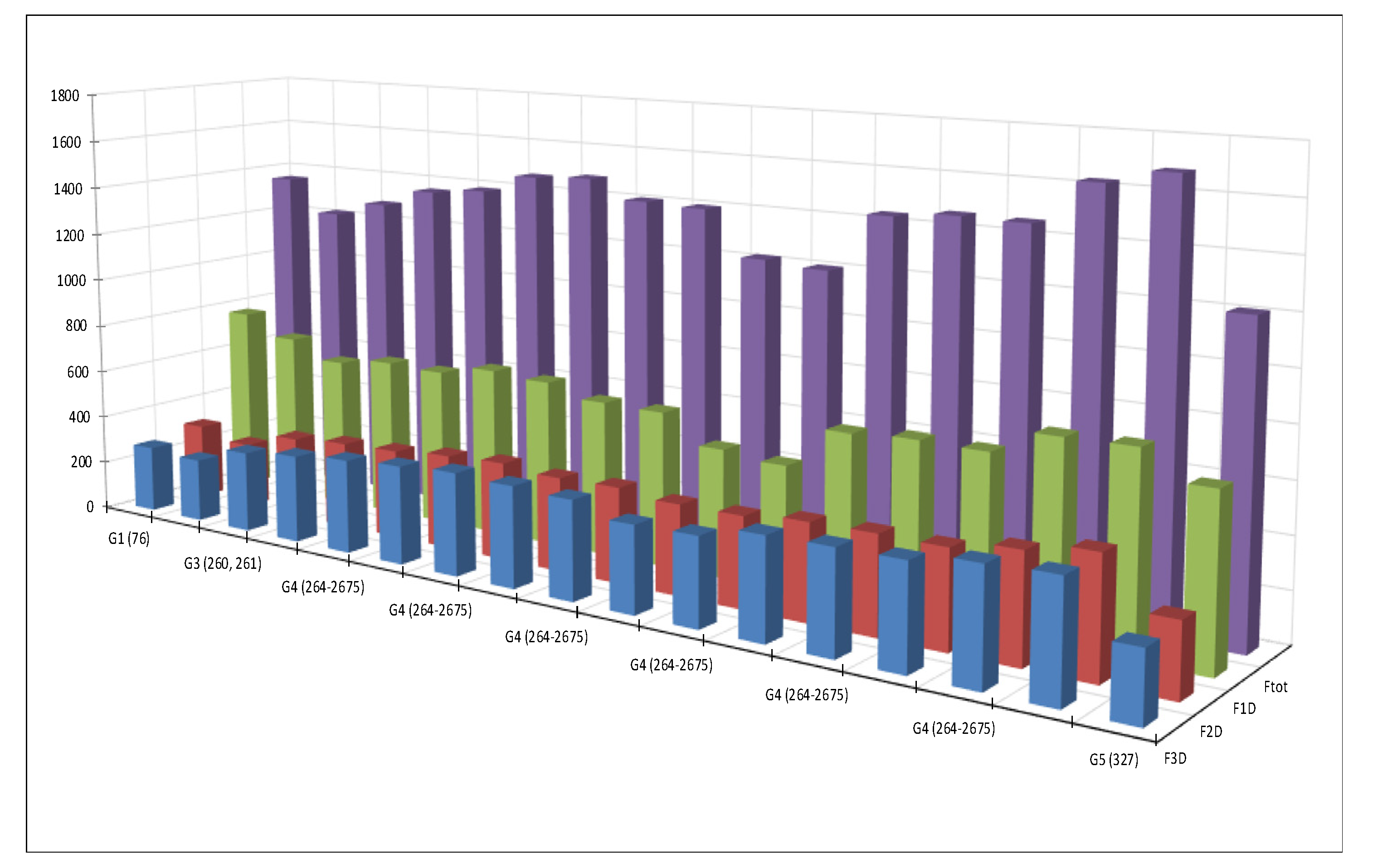
| F1D m3/Day | F2D m3/Day | F3D m3/Day | Total (Qd) m3/Day | |
|---|---|---|---|---|
| Minimum | 100 | 197 | 51 | 414 |
| Maximum | 772 | 462 | 454 | 1680 |
| Average | 442 | 251 | 197 | 890 |
| Standard deviation | 143 | 33 | 59 | 219 |
| Day | Group | Qd (m3/Day) | Qd-Average (m3/Day) |
|---|---|---|---|
| 76 | G1 (76) | 1354 | 464 |
| 86 | G2 (86) | 1216 | 326 |
| 260 | G3 (260. 261) | 1280 | 390 |
| 261 | G3 (260. 261) | 1357 | 467 |
| 264 | G4 (264–2675) | 1383 | 493 |
| 265 | G4 (264–2675) | 1463 | 573 |
| 266 | G4 (264–2675) | 1477 | 587 |
| 267 | G4 (264–2675) | 1404 | 514 |
| 268 | G4 (264–2675) | 1396 | 506 |
| 269 | G4 (264–2675) | 1217 | 327 |
| 270 | G4 (264–2675) | 1201 | 311 |
| 271 | G4 (264–2675) | 1435 | 545 |
| 272 | G4 (264–2675) | 1459 | 569 |
| 273 | G4 (264–2675) | 1455 | 565 |
| 274 | G4 (264–2675) | 1624 | 734 |
| 275 | G4 (264–2675) | 1680 | 790 |
| 327 | G5 (327) | 1208 | 318 |
| Day | Groupe | FL3 (%) | FL2 (%) | FL1 (%) |
|---|---|---|---|---|
| 76 | G1 (76) | 20 | 23 | 57 |
| 86 | G2 (86) | 21 | 22 | 57 |
| 260 | G3 (260, 261) | 26 | 26 | 48 |
| 261 | G3 (260, 261) | 26 | 26 | 48 |
| 264 | G4 (264–2675) | 28 | 26 | 46 |
| 265 | G4 (264–2675) | 27 | 26 | 47 |
| 266 | G4 (264–2675) | 28 | 27 | 45 |
| 267 | G4 (264–2675) | 29 | 27 | 44 |
| 268 | G4 (264–2675) | 28 | 27 | 44 |
| 269 | G4 (264–2675) | 28 | 29 | 42 |
| 270 | G4 (264–2675) | 29 | 30 | 41 |
| 271 | G4 (264–2675) | 28 | 27 | 46 |
| 272 | G4 (264–2675) | 28 | 26 | 46 |
| 273 | G4 (264–2675) | 28 | 26 | 46 |
| 274 | G4 (264–2675) | 27 | 26 | 47 |
| 275 | G4 (264–2675) | 27 | 27 | 45 |
| 327 | G5 (327) | 22 | 23 | 55 |
Publisher’s Note: MDPI stays neutral with regard to jurisdictional claims in published maps and institutional affiliations. |
© 2021 by the authors. Licensee MDPI, Basel, Switzerland. This article is an open access article distributed under the terms and conditions of the Creative Commons Attribution (CC BY) license (https://creativecommons.org/licenses/by/4.0/).
Share and Cite
Mashhadi, N.; Shahrour, I.; Attoue, N.; El Khattabi, J.; Aljer, A. Use of Machine Learning for Leak Detection and Localization in Water Distribution Systems. Smart Cities 2021, 4, 1293-1315. https://doi.org/10.3390/smartcities4040069
Mashhadi N, Shahrour I, Attoue N, El Khattabi J, Aljer A. Use of Machine Learning for Leak Detection and Localization in Water Distribution Systems. Smart Cities. 2021; 4(4):1293-1315. https://doi.org/10.3390/smartcities4040069
Chicago/Turabian StyleMashhadi, Neda, Isam Shahrour, Nivine Attoue, Jamal El Khattabi, and Ammar Aljer. 2021. "Use of Machine Learning for Leak Detection and Localization in Water Distribution Systems" Smart Cities 4, no. 4: 1293-1315. https://doi.org/10.3390/smartcities4040069