Abstract
(1) Problem Statement: The development of clustering algorithms for neural recordings has significantly evolved, reaching a mature stage with predominant approaches including partitional, hierarchical, probabilistic, fuzzy logic, density-based, and learning-based clustering. Despite this evolution, there remains a need for innovative clustering algorithms that can efficiently analyze neural spike data, particularly in handling diverse and noise-contaminated neural recordings. (2) Methodology: This paper introduces a novel clustering algorithm named Gershgorin—nonmaximum suppression (G–NMS), which incorporates the principles of the Gershgorin circle theorem, and a deep learning post-processing method known as nonmaximum suppression. The performance of G–NMS was thoroughly evaluated through extensive testing on two publicly available, synthetic neural datasets. The evaluation involved five distinct groups of experiments, totaling eleven individual experiments, to compare G–NMS against six established clustering algorithms. (3) Results: The results highlight the superior performance of G–NMS in three out of five group experiments, achieving high average accuracy with minimal standard deviation (SD). Specifically, in Dataset 1, experiment S1 (various SNRs) recorded an accuracy of 99.94 0.01, while Dataset 2 showed accuracies of 99.68 0.15 in experiment E1 (Easy 1) and 99.27 0.35 in experiment E2 (Easy 2). Despite a slight decrease in average accuracy in the remaining two experiments, D1 (Difficult 1) and D2 (Difficult 2) from Dataset 2, compared to the top-performing clustering algorithms in these categories, G–NMS maintained lower SD, indicating consistent performance. Additionally, G–NMS demonstrated robustness and efficiency across various noise-contaminated neural recordings, ranging from low to high signal-to-noise ratios. (4) Conclusions: G–NMS’s integration of deep learning techniques and eigenvalue inclusion theorems has proven highly effective, marking a significant advancement in the clustering domain. Its superior performance, characterized by high accuracy and low variability, opens new avenues for the development of high-performing clustering algorithms, contributing significantly to the body of research in this field.
1. Introduction
Extracellular electrophysiology is a key method in neuroscience for recording brain activity, as detailed in [1]. With this technique, the electrodes are placed in the brain’s cortex, and the action potentials, or “spikes”, are recorded from nearby neurons. Through this technique, researchers can gain access in real time to the brain activities. However, the challenge lies in the noisy nature of brain signals and the presence of multiple spikes from adjacent neurons, which make it difficult to determine the specific source of each spike. To address this issue, researchers have developed spike-sorting algorithms that categorize these spikes into distinct clusters or classes. Traditionally, these algorithms consist of a series of stages: filtering raw data, detection of spikes, feature extraction of dominant features, and, finally, clustering of spikes according to their specific features [2]. Current research methods enhance these stages by incorporating new algorithms at each step. However, the effectiveness of spike sorting still largely depends on the clustering method’s ability to separate different spikes efficiently. Within this research, the main focus will be on developing a new clustering algorithm to improve this aspect.
Clustering algorithms, established and utilized for decades, are fundamental in data analysis [3]. The K-means algorithm, a well-recognized method introduced by MacQueen et al. in 1967 [4] and later applied to spike sorting in 1988, is a prime example [5]. In K-means clustering, one can select the number of clusters (K) and initialize centroids within the data points. These centroids are then adjusted iteratively to minimize variance within each cluster. Despite its long-standing use and simplicity, the K-means algorithm faces challenges, particularly in initializing the centroids correctly and determining the right number of clusters, which can lead to inaccurate results. In addition to that, it is not applicable for unsupervised clustering. However, it remains a popular method in spike sorting, with various adaptations [6,7].
In contrast to traditional K-means algorithm, the fuzzy C-means (FCM) algorithm was developed by Bezdek et al. [8] in 1984, and offers a different approach based on soft computing. FCM allows data points to belong to several clusters, each with varying degrees of membership. The membership level of each data point is assigned as 0 or 1, where 1 indicates that the data point is closer to the centroid of the cluster and 0 indicates that the data point is far from the cluster centroid point. The algorithm’s goal is to minimize the weighted sum of the squared distances from each data point to its respective cluster center, where the weights are based on the membership levels. In 2000, Zouridakis et al. [9] presented the first FCM application for spike sorting. Subsequently, various enhanced versions of FCM have been introduced for the clustering applications mentioned in [10].
The DBSCAN (density-based spatial clustering) [11] offers a density-based clustering alternative. DBSCAN, unlike K-means, does not require users to predefine the number of clusters. It determines clusters by estimating the local density of data points, relying mainly on two parameters: “epsilon”, a distance threshold, and “Minpts”, the minimum number of points needed for a dense region. In DBSCAN, clusters are formed by examining all data points within an epsilon distance of an arbitrary point and meeting the Minpts criteria. DBSCAN is known for its robustness against outliers, though selecting the appropriate “epsilon” and “Minpts” values remains a challenge.
Similarly, Campello et al. [12] introduced HDBSCAN (hierarchical density-based spatial clustering), an extension of DBSCAN. HDBSCAN, like DBSCAN, identifies clusters based on the density of data points but adds a hierarchical structure based on varying density levels, allowing for more refined cluster selection by the user. A significant advantage of HDBSCAN over DBSCAN is its ability to manage clusters of varying densities. Agglomerative clustering [13] is another hierarchical clustering method. Employing a bottom-up strategy, it starts with each data point as a separate cluster and then merges them based on their proximity, forming a hierarchical structure. This process continues until all points are combined into a single cluster or a predetermined level is reached. Agglomerative clustering, while effective, is computationally intensive for larger datasets and is sensitive to noise and outliers, which can lead to misinterpretation of cluster structures. The Isotonic Splitting (ISO-SPLIT) clustering algorithm, developed by Magland et al. [14] in 2015, addresses the specific challenges of clustering high-dimensional data. It uses isotonic regression to automatically determine the best number of clusters and adjusts them iteratively based on statistical tests that evaluate the likelihood of data points belonging to the same cluster.
Algorithms like K-means and DBSCAN are well-established methodologies that have evolved over a significant period. Despite their long-standing presence, these state-of-the-art methods are still utilized in contemporary comparative studies of novel research [15]. In contrast to basic clustering algorithms, recent advancements in the field have led to the development of sophisticated spike-sorting algorithms, including KiloSort [16] and Spysort [17]. These innovative tools are capable of supporting large-scale analyses of multichannel neural recordings and have shown promising accuracy in spike-sorting tasks [18]. However, their potential impact and methodological advancements have not been extensively considered in literature reviews or comparative studies. The current focus tends to be narrowly centered on the clustering aspect of spike sorting, overlooking the broader potential of these advanced tools.
Beyond traditional clustering methods that utilize statistical techniques such as hierarchical, probabilistic, fuzzy, and density-based methods, this paper makes the following contributions:
- Introduces a novel neural signals clustering algorithm, referred to as G–NMS, which integrates geometric principles through the Gershgorin circle theorem [19] and incorporates the nonmaximum suppression (NMS) algorithm [20].
- Demonstrates the robustness and efficiency of G–NMS across various noisy neural recordings, ranging from low to high SNRs.
- Highlights the effective integration of deep learning techniques and eigenvalue inclusion theorems in G–NMS, marking a significant advancement in the clustering domain and contributing significantly to the body of research in this field.
Figure 1 outlines the comprehensive framework of the proposed G–NMS clustering algorithm. This paper is structured as follows: Section 2, Materials and Methods, provides a detailed explanation of each step of the proposed method and includes a description of the dataset used for testing and comparison. Section 3, Results and Discussion, presents a comprehensive explanation of the results and discusses how the performance of the proposed method varies with changing parameters. Finally, Section 4 concludes the paper by summarizing the findings, highlighting the limitations, and suggesting potential future research directions.
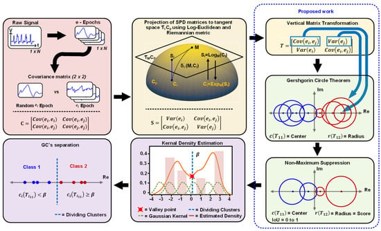
Figure 1.
Overview of G–NMS clustering framework for neural spike clustering. The workflow begins with raw signal processing (left panel) and covariance metric calculation. The (central panel) shows the projection of SPD matrices to target space using Log-Euclidean and Riemannian metrics. The (right middle panel) depicts the vertical matrix transformation and Gershgorin Circle Theorem application. Non-Maximum Suppression is applied (bottom right panel) to enhance separation. Kernel Density Estimation (bottom central panel) visualizes estimated density for cluster identification. The (bottom left panel) illustrates the separation of GC’s into Class 1 (red) and Class 2 (blue).
2. Materials and Methods
2.1. Methodology
2.1.1. Preprocessing
In the initial preprocessing stage, the raw recording undergoes min–max normalization, where 1… represents the datapoints. This technique rescales the values to a standardized range between 0 and 1. After normalization, raw signals are segmented into shorter times series, called epochs (e). In this study, each epoch is fixed at 56 data points (N) as .
2.1.2. Covariance Matrices
After the preprocessing phase, the principal clustering procedure begins with the calculation of the sample covariance matrix (SCM) between two epochs, as depicted in Figure 1. Initially, a random epoch is selected from a set of e-epochs; subsequently, the covariance matrix is computed relative to the remaining e-epochs. The method to determine the covariance between a randomly selected epoch and is presented in Equation (1).
where:
and = Individual data points of and at time ;
and = Sample mean of and .
The SCM is expressed as follows:
where:
= ;
= .
2.1.3. Projection of Covariance Matrices to Tangent Plane
Inherently possessing the attributes of symmetric positive definite (SPD), the SCM matrices , of dimensions , are of full rank and nonsingular. If the space of SCM matrices is equipped with a differential structure, it becomes a Riemannian manifold , defined as
Figure 2 represents the mapping of a Riemannian space of a geodesic path to tangent space. It illustrates the projection of points and from the Riemannian manifold to tangent space, with the reference point transformed into the null matrix , which serves as the origin of . As shown in Figure 2, the Riemannian manifold space is nonlinear, and SPD matrices inherently belong to a non-Euclidean domain. To accurately map the datapoints of an SCM on a Riemannian manifold to tangent space , the log-Euclidean kernel is utilized.
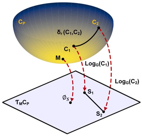
Figure 2.
Illustration of geodesic path and logarithm mapping from Riemannian manifold to tangent space. The projection of SPD matrices and from the curved manifold to the tangent space . The geodesic distance between and on the manifold is depicted by the solid black line. The Log-Euclidean mapping of and to points and in the tangent space is shown with red dashed arrows. represents the mean point on the manifold, while is the origin in the tangent space.
For every point M on manifold Cp, the transformation to the tangent space is defined as
The selection of an appropriate reference point is crucial for projecting datapoints into . In this study, the Riemannian mean , calculated using Equation (2) [21], serves as the reference point for the manifold.
Riemannian distances between two SPD matrices and are defined as follows:
The transformed SCM matrix is then represented as matrix :
2.1.4. Vertical Matrix Transformation
After transformation of the datapoints into the tangent space, each projected SCM matrix undergoes into a vertical flip to form matrix :
This transformation aligns the variance of and along the off-diagonal axis and their covariance along the diagonal axis. Such a distinctive transformation facilitates the application of the Gershgorin circle theorem, generating Gershgorin circles (GCs) of varying radii. The necessity for this transformation is further explained in the following section.
2.1.5. Gershgorin Circle Theorem
The Gershgorin circle theorem has been widely applied in various fields, including feature extraction of signal and images [22,23] and grid stability analysis [24]. The Gershgorin circle theorem estimates the eigenvalue inclusion of any square matrix . It generates the sets of GCs with a radius and center from a given matrix . Hence, the union of all GCs includes the estimate location of eigenvalues of matrix . The GC theorem states that each eigenvalue of matrix L is contained within at least one GC. Given an square matrix with elements , the GC radius and center for each row element are defined by Equations (3) and (4), respectively.
The is the absolute sum of the off-diagonal elements of row , and is the diagonal element of row . Figure 1 visualizes the implementation of the GC theorem on the vertically flipped matrix , by extracting the first row GC radius , which is equal to , and center , which is equal to elements. The primary reason for focusing solely on the first row of GC for clustering is that it encompasses the variance and covariance of all epochs in relation to a chosen epoch . This approach effectively captures the relationship between the epochs, making the first row pivotal datapoints for clustering analysis. Figure 3 demonstrates the benefits of vertical matrix transformation. For instance, implementation of the GC theorem on matrix (shown in Figure 3a) fails to identify two distinct spikes (GCs), whereas on matrix (shown in Figure 3b), the two spikes (GCs) are effectively segregated.
2.1.6. Nonmaximum Suppression
The nonmaximum suppression (NMS) is an algorithm which is generally utilized in the field of computer vision for object detection tasks. Generally, the NMS algorithm is implemented to suppress the bounding boxes and eliminate the redundant boxes. However, within this study, the circle-based NMS is implemented instead using of bounding boxes. As the datapoint or number of epochs increases, the number of GC circles also increases, which potentially results in misclassification and therefore decreases the clustering accuracy. Therefore, to reduce the occurrence of overlapping circles, NMS is applied to each GC. Figure 4a,b visualizes the before and after effect of NMS on the implementation on GCs with intersection over union (IoU) of 0.1 for two different classes with a total of 4000 epochs.
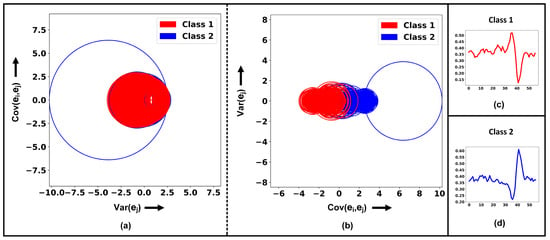
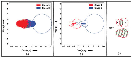

Figure 3.
Comparative analysis of class separation pre- and post-vertical matrix transformation. (a) displays Gershgorin circles pre-transformation, centered at with radii (b) shows post-transformation Gershgorin circles, now centered at and radius . Subplots (c,d) depict visual representations of random neural spikes for Class 1 and Class 2, respectively.

Figure 4.
Gershgorin circle theorem application and intersection quantification. (a) Overlapping Gershgorin circles for Class 1 and Class 2 before nonmaximum suppression (NMS). (b) Separation of classes using NMS. (c) The calculation of intersection measure (IoU) between circles A and B, illustrating the degree of overlap. The numerator represents the intersection area between the circles, and the denominator (green lines) represents the union of areas A and B.
In the NMS procedure, each GC is assigned a score corresponding to the of matrix . An IoU value , ranging between 0 and 1, is selected to determine the extent of overlap or interaction between two GCs. Assume that there is GC with center and radius and GC with center and radius , as shown in Figure 4c. The algorithm initiates with the identification of the GC with the highest score; assume that GC is the one with the highest score. Then, the subsequent calculations determine the distance between the and as follows:
If the , then the circles do not overlap and the IoU is zero. In cases of overlap, as depicted in Figure 4c, the IoU between GCs and is computed using Equation (5). If exceeds , GC is suppressed, under the presumption that GC possesses a higher score. This iterative process prioritizes GCs based on their scores, suppressing those that significantly overlap with a higher-scored GC. Note that the relevant GC centers are preserved in the vector .
where:
2.1.7. Kernel Density Estimation
After the NMS phase, which effectively segregates the GCs into two visually distinct clusters, as shown in Figure 4b, kernel density estimation (KDE) is employed on the reduced GC set. The kernel density estimation (KDE) is a statistical nonparametric approach for estimating the probability density function (PDF) of a random variable. The KDE is computed for using Equation (6) [25].
where:
= The estimated density at point ;
= The number of datapoints;
= The datapoints;
= The Gaussian kernel functions;
= The bandwidth of kernel function.
The KDE of based on the Gaussian kernel with appropriate bandwidth is shown in Figure 1. The bandwidth parameter controls the smoothness of the density estimation in such a way that a low bandwidth may yield a noisy estimation, whereas a high bandwidth could overly smooth the data, potentially leading to underfitting. The bandwidth is typically chosen within the range of 0.0 to 1.0, based on the signal-to-noise ratio (SNR) of the spikes or signal.
Subsequent to KDE, the local maxima and minima are identified within the distribution. During this process, the global minimum is located within the estimated density function, which is then labeled as the “primary valley” in the distribution. With the location of the primary valley in distribution, the datapoints are segmented or clustered. As illustrated in Figure 1, the x-coordinate corresponding to the primary valley is established as the threshold value . This threshold is then applied to segment the clusters into two subsets. The segmentation of a subsets and is performed based on GCs’ centers conditions:
2.2. Datasets
This study utilized two publicly available synthetic datasets, each characterized by distinct neural spike shapes or spike classes. Table 1 presents a structured overview of the different experiments conducted as part of the performance evaluation. For each experiment, the table lists the dataset that is used and the corresponding number of epochs for each spike class during the clustering process. The selection of spike classes for each dataset was random, and it was ensured that the chosen classes were distinct.

Table 1.
Experimental groupings and epoch counts for two datasets with various signal-to-noise ratios (SNRs) and neural spike classes (Spk) combinations.
2.2.1. Dataset 1
Dataset 1 is composed of synthetic, simulated action potentials that are superimposed with additive Gaussian noise [26]. The synthetic data are generated according to the equation from [27]:
It is simulating action potentials, with parameters (), which is described in great detail in [26]. The dataset includes seven different signal-to-noise ratios (SNRs), namely, 0.5, 0.75, 1.0, 1.25, 1.50, 1.75, and 2.0, with each number representing “σ” of the Gaussian noise. The dataset comprises sets of three action potentials, each with unique shapes and properties, labeled as Spk1, Spk2, and Spk3. For this study, only three SNR sets were chosen for experimentation: 0.5, 1.25, and 2.0, allowing for a focused analysis on specific noise conditions. The samples in Dataset 1 are generated at a sampling frequency of 20 kHz, so that it is reflecting a mean firing rate of 3.3 Hz, which closely aligns with real-world neural signal characteristics. For each of the SNR-based experiments, a random selection process is employed to choose two distinct spike classes for analysis. Each SNR set comprises ten recordings, each lasting 200 s, and provides a substantial amount of data for analysis. The numbers of epochs for each class within each SNR set are detailed in Table 1. Furthermore, the size of each epoch is standardized to 56 samples, and the preprocessed segmented dataset was used from [28]. Each epoch of 56 samples captures a complete neural spike (action potential). All experiments conducted using various signal-to-noise ratios (SNRs) from Dataset 1 are collectively grouped under the label “S1”.
2.2.2. Dataset 2
Dataset 2 features the widely used synthetic neural dataset known as Wave_Clus [29]. The dataset is subdivided into four distinct categories, allowing varying levels of complex experiments in spike sorting. The categories are labeled as Easy 1 (E1), Easy 2 (E2), Difficult 1 (D1), and Difficult 2 (D2), so that each one offers a unique challenge for the clustering algorithm. Each of the subdatasets is characterized by four different signal-to-noise ratios (SNRs): 0.05, 0.10, 0.15, and 0.20. The recordings within these datasets have a sampling frequency set to 24 kHz. Each subdataset consists of three different types of spikes, labeled as Spk1, Spk2, and Spk3. For this study, the easiest and the most challenging subdatasets were selected for experiments, specifically the ones with SNRs of 0.05 and 0.20. This selection criterion was aimed at testing the clustering algorithm’s capabilities at the extremes of the noise spectrum. Furthermore, in alignment with the methodology applied to Dataset 1, each experiment within Dataset 2 also involves the random selection of two spike classes. The total number of samples in each epoch for Dataset 2 is 56.
3. Results and Discussion
This study presents a comparative analysis of the G–NMS clustering method against six established algorithms, utilizing a total of eleven experimental trials—three from Dataset 1 and eight from Dataset 2. All experiments were performed on a university supercomputer equipped with 20 cores and 20 GB of RAM per core to ensure consistency and reliability in the experimental setup. To evaluate the efficacy of the clustering algorithms, two distinct metrics were employed: adjusted mutual information (AMI) and accuracy (ACC). These metrics were calculated by comparing the clustering results with the ground truth labels. The AMI metric assesses the correlation between the ground truth and the predicted clusters by measuring mutual information, reflecting the knowledge gained about one variable by observing another. An AMI score of 1 indicates perfect alignment with the ground truth, while a score of 0 implies no correlation. The ACC ranges between 0 to 100 percent.
Figure 5 presents the AMI scores for each experiment across various clustering algorithms. In the first dataset, for the experiment labeled “SNR0.5_Spk-1,2”, K-means and G–NMS achieved the highest AMI, scoring an impressive highest AMI of 0.991. In comparison, agglomerative clustering reached an AMI of 0.906. In scenarios with moderate noise in spike, such as “SNR1.25_Spk-2,3”, G–NMS excelled with a score of 0.992, outperforming other methods. Notably, agglomerative, HDBSCAN, DBSCAN, and FCM methods faced challenges, reflected by significantly lower AMI scores, indicating difficulties in specific clustering tasks. In experiments with higher noise levels, “SNR2.0_Spk-3,1”, G–NMS showed robust performance with an AMI score of 0.993, which is slightly lesser than K-means. Other methods, including HDBSCAN and DBSCAN, achieved relative improvements with AMI scores of 0.653 and 0.763, respectively, outpacing agglomerative and FCM in performance.
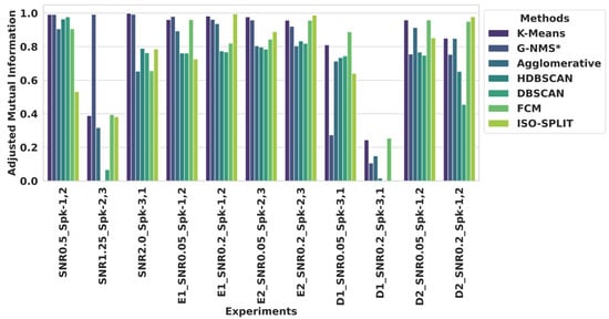
Figure 5.
Evaluation of clustering algorithms using adjusted mutual information. The bar graph compares the adjusted mutual information scores of seven clustering methods—K-means, G–NMS*, agglomerative, HDBSCAN, DBSCAN, FCM, and ISO-SPLIT—across various experimental scenarios characterized by different SNR levels and neural spike class (Spk) pairings.
For Dataset 2, in the Easy—1 category, G–NMS recorded AMI scores of 0.979 and 0.962 for “E1_SNR0.2_Spk-1,2” and “E1_SNR0.05_Spk-1,2”, respectively. Interestingly, in the “E1_SNR0.05_Spk-1,2” trial, G–NMS led the performance, whereas ISO-SPLIT edged ahead in “E1_SNR0.2_Spk-1,2” with a slightly higher AMI of 0.994. Similar patterns emerged in the Easy—2 categories; K-means demonstrated robust performance with an AMI of 0.977 in “E2_SNR0.05_Spk-2,3”, slightly surpassing G–NMS, which scored 0.958. The other algorithms varied in efficacy, with agglomerative clustering at 0.804, HDBSCAN at 0.797, DBSCAN at 0.785, FCM at 0.844, and ISO-SPLIT at 0.889, with ISO-SPLIT showing a commendable improvement compared to certain traditional methods.
In the Difficult 1 category of Dataset 2, all algorithms faced challenges in clustering, particularly in “D1_SNR0.2_Spk-3,1”. However, in “D1_SNR0.05_Spk-3,1”, FCM led with an AMI of 0.888, followed by K-means at 0.810, while G–NMS scored 0.274. Agglomerative clustering, HDBSCAN, and DBSCAN registered AMI scores of 0.713, 0.734, and 0.745, respectively.
The Difficult 2 categories presented another difficult challenge for clustering spikes, with “D2_SNR0.05_Spk-1,2” showing K-means with the highest AMI of 0.959, affirming its clustering capabilities. Agglomerative clustering, FCM, and ISO-SPLIT also displayed strong performances with AMI scores of 0.914, 0.959, and 0.852, respectively. In contrast, G–NMS had a lower AMI of 0.756. In the “D2_SNR0.2_Spk-1,2” experiment, K-means maintained high performance with an AMI of 0.850, and ISO-SPLIT surpassed with the highest AMI of 0.978. Meanwhile, G–NMS performance just had an AMI of 0.753. Agglomerative closely paralleled K-means with an AMI of 0.849. HDBSCAN and DBSCAN saw a decrease in performance, scoring 0.652 and 0.455, respectively, highlighting the complexity of clustering in noisy conditions.
Figure 6 showcases the accuracy (ACC) performance for each experiment across the various clustering methods. Complementing this, Figure 7 provides a statistical overview, displaying the average ACC and standard deviation (SD) for each trial within Dataset 1. The table further breaks down the performance by difficulty level, offering a comparison of the average ACC and SD for two trials each in Easy 1 (E1), Easy 2 (E2), Difficult 1 (D1), and Difficult 2 (D2) within Dataset 2. This dual presentation of results in both graphic and tabular form allows for a comprehensive analysis of the clustering methods’ performance. Examining further the specifics of clustering ACC performance, the G–NMS method stood out in the S1 category with an impressive ACC of 99.94% and a notably low SD of 0.01, highlighting its exceptional precision and reliability. K-means also performed well, achieving a 94.40% ACC, but with a higher SD of 9.64, its results were less consistent. Agglomerative clustering and FCM exhibited moderate accuracy levels, scoring 88.11% and 91.65%, respectively, yet their higher SDs suggest greater variability in their results. HDBSCAN and DBSCAN presented lower ACCs and greater inconsistencies, particularly HDBSCAN, with a significantly lower ACC of 75.66% and a high SD of 34.67. ISO-SPLIP trailed with the least effectiveness, attaining only a 47.52% ACC and a high SD of 26.92.
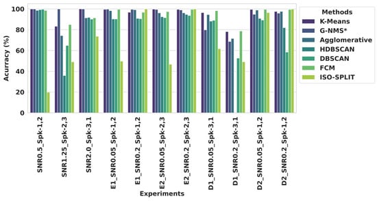
Figure 6.
Algorithmic accuracy in cluster analysis across diverse experimental conditions. The bar chart demonstrates comparable accuracy of various clustering algorithms, including K-means, G–NMS*, agglomerative, HDBSCAN, DBSCAN, FCM, and ISO-SPLIT, as applied to different experiments with specific SNR values and neural spike class (Spk) combinations.
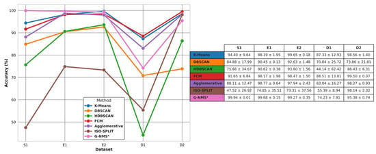
Figure 7.
Average accuracy of clustering algorithms across experimental groupings. The line graph and inset table detail the performance of seven clustering techniques (K-means, DBSCAN, HDBSCAN, FCM, agglomerative, ISO-SPLIT, and G–NMS*) across experimental groupings (S1, E1, D1, D2). The table provides numerical values for average accuracy and standard deviation, reflecting the consistency and variability of each method within the respective groups.
In the E1 category, the G–NMS method maintained its superior performance, securing an ACC of 99.68% and an SD of 0.15, reaffirming its efficiency and consistency. K-means showed a closely competitive ACC of 98.19% and an SD of 1.95, while agglomerative clustering achieved an ACC of 98.77% with an SD of 0.64. FCM was slightly less accurate at 98.17%. HDBSCAN and DBSCAN demonstrated significant progress from their S1 performance, with both surpassing the 90% ACC mark. ISO-SPLIP, however, continued to underperform, with an ACC of 74.85% and a high SD of 35.51.
The E2 category saw the G–NMS method lead narrowly with a 99.27% ACC and a minimal SD of 0.15. K-means and agglomerative clustering also exhibited strong performances, with ACCs of 98.65% and 97.94%, respectively. FCM posted an ACC close to that of K-means at 98.47%. HDBSCAN and DBSCAN, while improved, did not reach the top-tier accuracies. ISO-SPLIP remained the least effective, with a 73.31% ACC and a high SD of 37.56.
In the D1 category, there was a notable shift in performance dynamics. The G–NMS method saw a decrease in ACC to 74.23% and an increase in SD to 7.91. K-means led this dataset with an 87.33% ACC and an SD of 12.93. FCM also showed strong performance with an 88.51% ACC and an SD of 13.81. Agglomerative clustering and DBSCAN recorded moderate accuracies of 83.03% and 70.84%, respectively. However, HDBSCAN and ISO-SPLIP struggled with both ACC and consistency, especially HDBSCAN with an ACC of 44.14% and a high SD of 62.42.
Finally, in the D2 category, FCM outperformed others, attaining the highest ACC of 99.50% and an impressively low SD of 0.07. The G–NMS method, while still performing well, did not match FCM’s ACC, posting a 95.38% ACC and an SD of 0.74. K-means and agglomerative clustering both exhibited high ACCs of 98.56% and 98.27%, respectively, with low SDs. HDBSCAN and DBSCAN, on the other hand, had lower ACCs and higher variability, with HDBSCAN achieving an ACC of 86.43% and DBSCAN 73.86%.
Overall, across both datasets, the G–NMS method consistently showed high performance in AMI and ACC, affirming its effectiveness in clustering with few exceptions in Dataset 2 Difficult 1 (D1) and slightly lagging in Difficult 2 (D2) spike clustering. Moreover, K-means also demonstrated strong and consistent results across all metrics. FCM’s performance, particularly in AMI and ACC, was noteworthy, especially in Dataset 2. The other methods exhibited varying levels of effectiveness, with some, like ISO-SPLIT, showing significant differences between the two datasets.
Table 2 serves as a comprehensive guide to the parameter configurations for the G–NMS algorithm, tailored for different experimental scenarios within the datasets. It specifically outlines the settings for two key parameters: the intersection over union (IoU, α) threshold and the bandwidth (h) of the Gaussian kernel. The IoU threshold is a crucial factor in the nonmaximum suppression (NMS) algorithm, effectively utilized for suppressing Gershgorin circles (GCs). Simultaneously, the bandwidth of the Gaussian kernel plays a pivotal role in accurately estimating the probability density function (PDF), integral to the algorithm’s performance.

Table 2.
Selection of IoU and kernel bandwidth parameters across SNR variants and their impact on clustering accuracy.
For instance, in the Dataset 1 experiments “SNR0.5_Spk-1,2”, “SNR1.25_Spk-2,3”, and “SNR2.0_Spk-3,1”, the IoU value is consistently set at 0.1, while the bandwidth varies from 0.4 to 0.1 as the noise (SNR) in the spikes increases, yet the ACC performance remains almost consistent. In contrast, for Dataset 2, both the IoU values and bandwidth are adjusted to achieve higher ACC performance. Notably, in the “D1_SNR0.2_Spk-3,1” experiment with the noisiest spikes, a lower bandwidth of 0.06 and an IoU of 0.4 were selected, but the ACC for G–NMS was still low, at 68.639%. In comparison, the “D2_SNR0.05_Spk-1,2” and “D2_SNR0.2_Spk-1,2” experiments, despite having different noise levels, maintained the same IoU at 0.4 and bandwidth at 0.1, resulting in higher ACCs of 94.855% and 95.907%, respectively. These results underscore the importance of optimal parameter selection based on the noise level in the input spikes. A higher noise level suggests the need for a lower bandwidth to capture finer changes in the distribution, while the IoU parameter should ideally range between 0.4 to 0.1 to ensure minimal yet effective suppression of Gershgorin circles (GCs). Selecting an IoU below 0.1 might result in too few GCs for effective kernel density estimation (KDE). The code and other supporting recourse for proposed method are available inside Supplementary Materials.
4. Conclusions
In conclusion, this paper introduces the innovative G–NMS clustering method, which uniquely employs the Gershgorin circle (GC) theorem in conjunction with the nonmaximum suppression (NMS) method, an approach that is not implemented in spike clustering applications. The empirical evaluations conducted with both datasets highlight the robust and excellent performance of the G–NMS method, characterized by minimal standard deviations, indicative of its reliability and consistency. While the G–NMS method consistently outperformed across most of the experimental setups, it is noteworthy that in the remaining two experiments—D1 and D2 from Dataset 2—the method experienced a modest decline in average accuracy. Specifically, there was a 14.28% and 4.12% decrease in accuracy for D1 and D2, respectively, when compared to the top-performing clustering algorithms in these categories. Despite this, G–NMS maintained lower standard deviations in these instances as well, underscoring its consistent performance across varying levels of complexity and noise. The observed dip in performance for D1 is attributed to reduced covariance between the two spike classes (Spk) involved in these particular datasets. This factor highlights the sensitivity of the G–NMS method to the inherent data characteristics, an aspect that may guide future optimizations and refinements of the algorithm.
The introduction of the G–NMS method represents a significant advancement in the field of clustering. It integrates the mathematical eigenvalue inclusion theorem (GC) and a post-processing object detection algorithm from the field of deep learning (NMS), opening new paths for exploration and application. Looking to the future, the performance of the G–NMS could be further enhanced by adopting a more robust covariance matrix instead of the sample covariance matrix currently in use. Additionally, exploring other eigenvalue inclusion theorems might offer a more precise estimation and localization of eigenvalues, thereby improving the algorithm’s accuracy.
Moreover, the algorithm’s effectiveness could be improved by incorporating a variant of the NMS algorithm, such as a soft-NMS approach, which might provide less rigid thresholding compared to the current hard-threshold, greedy NMS strategy. These potential modifications and enhancements to the G–NMS method hold promise for even more effective clustering solutions in future applications.
Supplementary Materials
The following supporting information can be downloaded at: https://www.mdpi.com/article/10.3390/signals5020020/s1. All code related to this work is available in [30].
Author Contributions
S.A.P. developed the approach for this research and drafted the manuscript. A.Y. helped to revise the drafted manuscript and provided valuable advice for this research. All authors have read and agreed to the published version of the manuscript.
Funding
This research received no external funding.
Data Availability Statement
All syntenic signal datasets supporting this study’s findings come from previously reported studies, which are cited accordingly within the manuscript.
Acknowledgments
We thank Rachel June Smith for her guidance and our reviewers for their helpful feedback on our manuscript.
Conflicts of Interest
The authors declare no conflicts of interest.
References
- Carter, M.; Shieh, J.C. Electrophysiology. In Guide to Research Techniques in Neuroscience; Academic Press: Cambridge, MA, USA, 2015. [Google Scholar]
- Rey, H.G.; Pedreira, C.; Quiroga, R.Q. Past, present and future of spike sorting techniques. Brain Res. Bull. 2015, 119, 106–117. [Google Scholar] [CrossRef] [PubMed]
- Lewicki, M.S. A review of methods for spike sorting: The detection and classification of neural action potentials. Netw. Comput. Neural Syst. 1998, 9, R53. [Google Scholar] [CrossRef]
- MacQueen, J. Some methods for classification and analysis of multivariate observations. In Proceedings of the Fifth Berkeley Symposium on Mathematical Statistics and Probability, Davis Davis, CA, USA, 27 December 1965–7 January 1966; University of California: Oakland, CA, USA, 1967; Volume 1, pp. 281–297. [Google Scholar]
- Salganicoff, M.; Sarna, M.S.L.; Gerstein, G.L. Unsupervised waveform classification for multi-neuron recordings: A real-time, software-based system. I. Algorithms and implementation. J. Neurosci. Methods 1988, 25, 181–187. [Google Scholar] [CrossRef] [PubMed]
- Chah, E.; Hok, V.; Della-Chiesa, A.; Miller, J.J.H.; O’Mara, S.M.; Reilly, R.B. Automated spike sorting algorithm based on Laplacian eigenmaps and k-means clustering. J. Neural Eng. 2011, 8, 016006. [Google Scholar] [CrossRef] [PubMed]
- Caro-Martín, C.R.; Delgado-García, J.M.; Gruart, A.; Sánchez-Campusano, R. Spike sorting based on shape, phase, and distribution features, and K-TOPS clustering with validity and error indices. Sci. Rep. 2018, 8, 17796. [Google Scholar] [CrossRef] [PubMed]
- Bezdek, J.C.; Ehrlich, R.; Full, W. FCM: The fuzzy c-means clustering algorithm. Comput. Geosci. 1984, 10, 191–203. [Google Scholar] [CrossRef]
- Zouridakis, G.; Tam, D.C. Identification of reliable spike templates in multi-unit extracellular recordings using fuzzy clustering. Comput. Methods Programs Biomed. 2000, 61, 91–98. [Google Scholar] [CrossRef] [PubMed]
- Nayak, J.; Naik, B.; Behera, H. Fuzzy C-means (FCM) clustering algorithm: A decade review from 2000 to 2014. In Computational Intelligence in Data Mining—Volume 2, Proceedings of the International Conference on CIDM, Bhubaneswar, India, 5–6 December 2015; Springer: Berlin/Heidelberg, Germany, 2015; pp. 133–149. [Google Scholar]
- Ester, M.; Kriegel, H.P.; Sander, J.; Xu, X. A density-based algorithm for discovering clusters in large spatial databases with noise. In KDD; AAAI: Washington, DC, USA, 1996; Volume 96, pp. 226–231. [Google Scholar]
- Campello, R.J.; Moulavi, D.; Sander, J. Density-based clustering based on hierarchical density estimates. In Knowledge Discovery and Data Mining, Proceedings of the Pacific-Asia Conference, Gold Coast, QLD, Australia, 14–17 April 2013; Springer: Berlin/Heidelberg, Germany, 2013; pp. 160–172. [Google Scholar]
- Ackermann, M.R.; Blömer, J.; Kuntze, D.; Sohler, C. Analysis of agglomerative clustering. Algorithmica 2014, 69, 184–215. [Google Scholar] [CrossRef]
- Magland, J.F.; Barnett, A.H. Unimodal clustering using isotonic regression: ISO-SPLIT. arXiv 2015, arXiv:1508.04841. [Google Scholar]
- Veerabhadrappa, R.; Hassan, M.U.; Zhang, J.; Bhatti, A. Compatibility evaluation of clustering algorithms for contemporary extracellular neural spike sorting. Front. Syst. Neurosci. 2020, 14, 34. [Google Scholar] [CrossRef]
- Pachitariu, M.; Steinmetz, N.; Kadir, S.; Carandini, M.; Kenneth, D.H. Kilosort: Realtime spike-sorting for extracellular electrophysiology with hundreds of channels. BioRxiv 2016, 061481. [Google Scholar] [CrossRef]
- Pouzat, C.; Detorakis, G.I. Spysort: Neuronal spike sorting with python. arXiv 2014, arXiv:1412.6383. [Google Scholar]
- Zhang, T.; Azghadi, M.R.; Lammie, C.; Amirsoleimani, A.; Genov, R. Spike sorting algorithms and their efficient hardware implementation: A comprehensive survey. J. Neural Eng. 2023, 20, 021001. [Google Scholar] [CrossRef] [PubMed]
- Gershgorin, S.A. Über die Abgrenzung der Eigenwerte einer Matrix. Izv. Akad. Nauk. SSSR 1931, 6, 749–754. [Google Scholar]
- Neubeck, A.; Van Gool, L. Efficient non-maximum suppression. In Proceedings of the 18th International Conference on Pattern Recognition, Hong Kong, China, 20–24 August 2006; Volume 3, pp. 850–855. [Google Scholar]
- Yger, F.; Berar, M.; Lotte, F. Riemannian approaches in brain-computer interfaces: A review. IEEE Trans. Neural Syst. Rehabil. Eng. 2016, 25, 1753–1762. [Google Scholar] [CrossRef]
- Patel, S.A.; Smith, R.; Yildirim, A. Gershgorin circle theorem-based featureextraction for biomedical signal analysis. Front. Neuroinformatics 2024, 18, 1395916. [Google Scholar] [CrossRef]
- Patel, S.A.; Yildirim, A. Overcoming Dimensionality Constraints: A Gershgorin Circle Theorem-Based Feature Extraction for Weighted Laplacian Matrices in Computer Vision Applications. J. Imaging 2024, 10, 121. [Google Scholar] [CrossRef] [PubMed]
- Xie, L.; Huang, J.; Tan, E.; He, F.; Liu, Z. The Stability Criterion and Stability Analysis of Three-Phase Grid-Connected Rectifier System Based on Gerschgorin Circle Theorem. Electronics 2022, 11, 3270. [Google Scholar] [CrossRef]
- Chen, Y. A tutorial on kernel density estimation and recent advances. Biostat. Epidemiol. 2017, 1, 161–187. [Google Scholar] [CrossRef]
- Bernert, M.; Yvert, B. An attention-based spiking neural network for unsupervised spike-sorting. Int. J. Neural Syst. 2019, 29, 1850059. [Google Scholar] [CrossRef]
- Adamos, D.A.; Kosmidis, E.K.; Theophilidis, G. Performance evaluation of PCA-based spike sorting algorithms. Comput. Methods Programs Biomed. 2008, 91, 232–244. [Google Scholar] [CrossRef] [PubMed]
- Patel, S.A.; Yildirim, A. Non-stationary neural signal to image conversion framework for image-based deep learning algorithms. Front. Neuroinformatics 2023, 17, 1081160. [Google Scholar] [CrossRef] [PubMed]
- Quiroga, R.Q.; Nadasdy, Z.; Ben-Shaul, Y. Unsupervised spike detection and sorting with wavelets and superparamagnetic clustering. Neural Comput. 2004, 16, 1661–1687. [Google Scholar] [CrossRef] [PubMed]
- Patel, S.A. G-NMS_Clustering [Sourecode]. 2024. Available online: https://github.com/sahaj432/G-NMS_Clustering.git (accessed on 13 February 2024).
Disclaimer/Publisher’s Note: The statements, opinions and data contained in all publications are solely those of the individual author(s) and contributor(s) and not of MDPI and/or the editor(s). MDPI and/or the editor(s) disclaim responsibility for any injury to people or property resulting from any ideas, methods, instructions or products referred to in the content. |
© 2024 by the authors. Licensee MDPI, Basel, Switzerland. This article is an open access article distributed under the terms and conditions of the Creative Commons Attribution (CC BY) license (https://creativecommons.org/licenses/by/4.0/).