
Voice Transformation Using Two-Level Dynamic Warping and Neural Networks


Abstract
:1. Introduction
2. Previous Voice Transformation Research
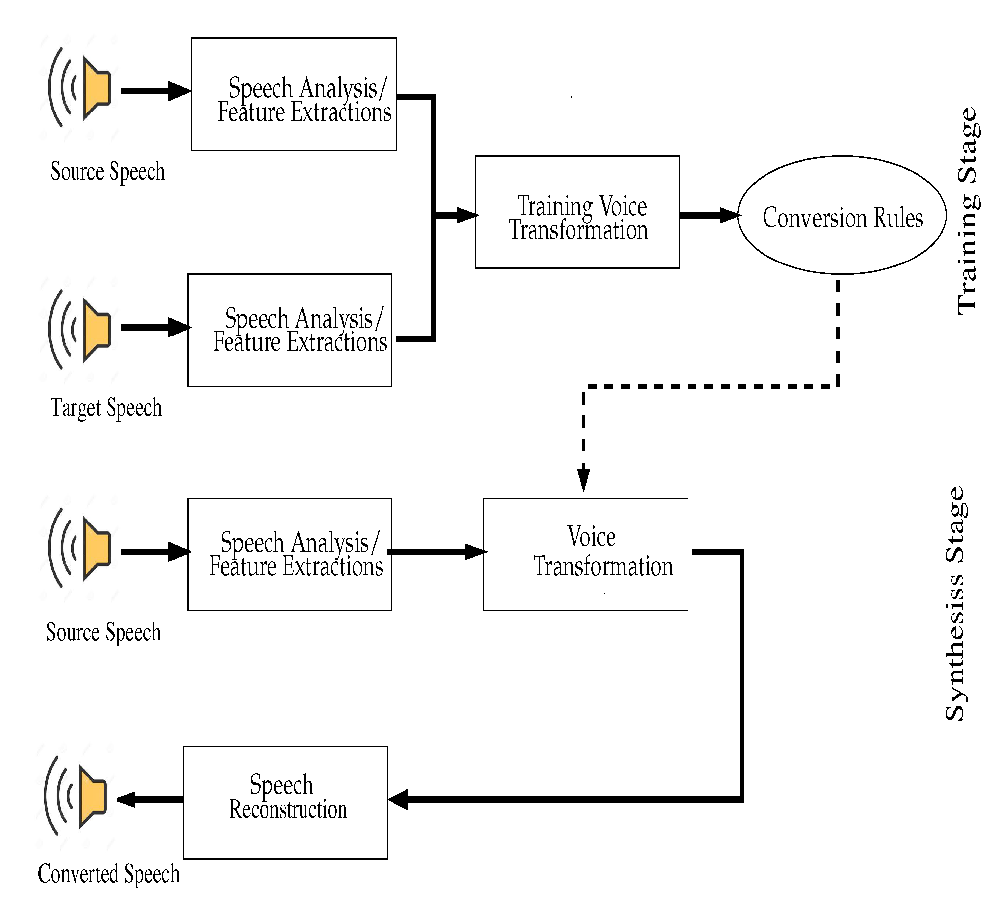
3. Voice Transformation Process
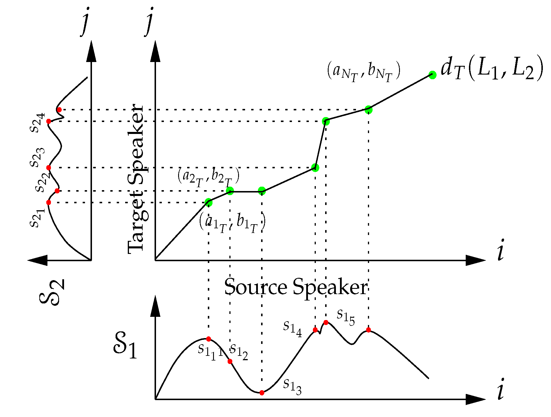
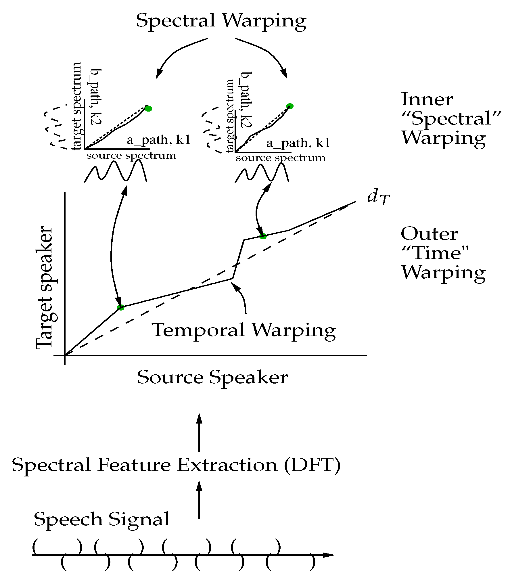
3.1. Two-Level Dynamic Warping
| Algorithm 1: Dynamic Warping () for Voice Transformation. |
| Input: First spectral sequence, Second spectral sequence, window size for DTW process window size for DFW process Output: Distance between and Indices and for temporal alignment Indices and for spectral alignment Begin Initialize DTW array, Initialize DFW array, Adapt window size, For For End For End For Set For For End For End For Set For For Adapt window size, For For , End For End For Searching minimum path through , save Minimum energy [ and ] , End For End For Searching minimum path through , save |
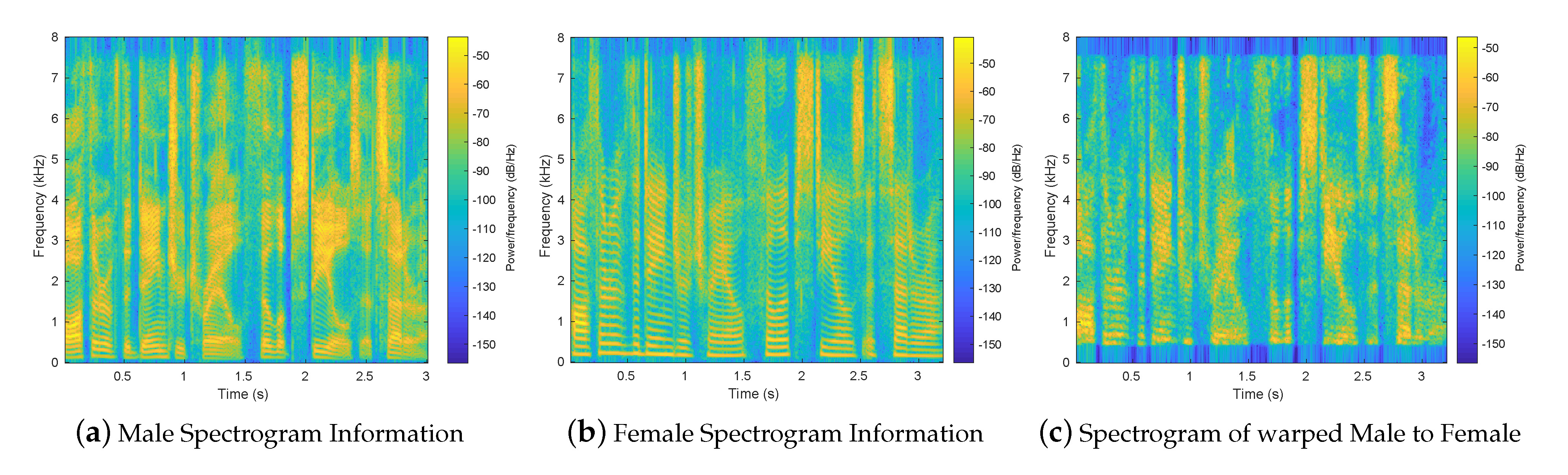
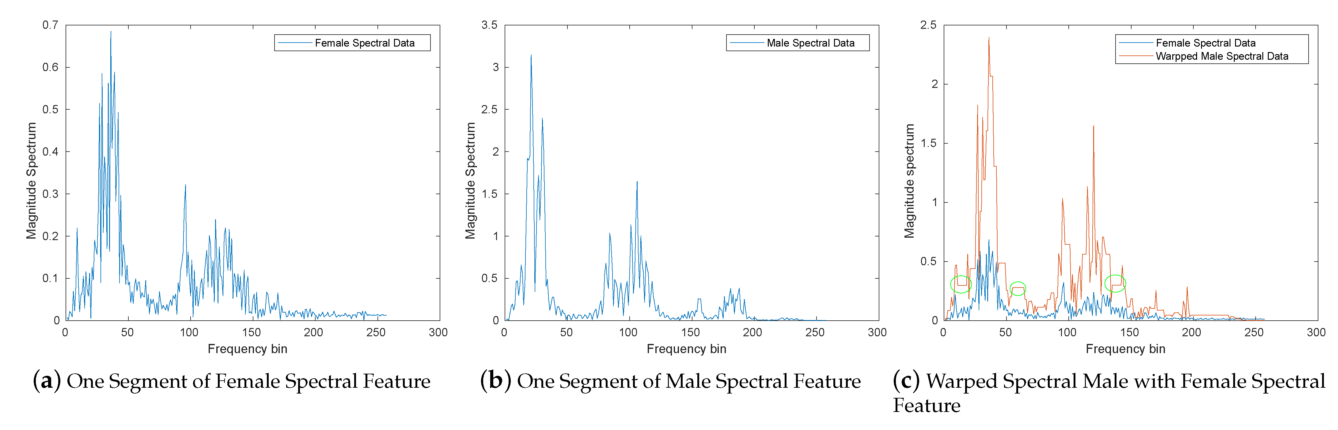
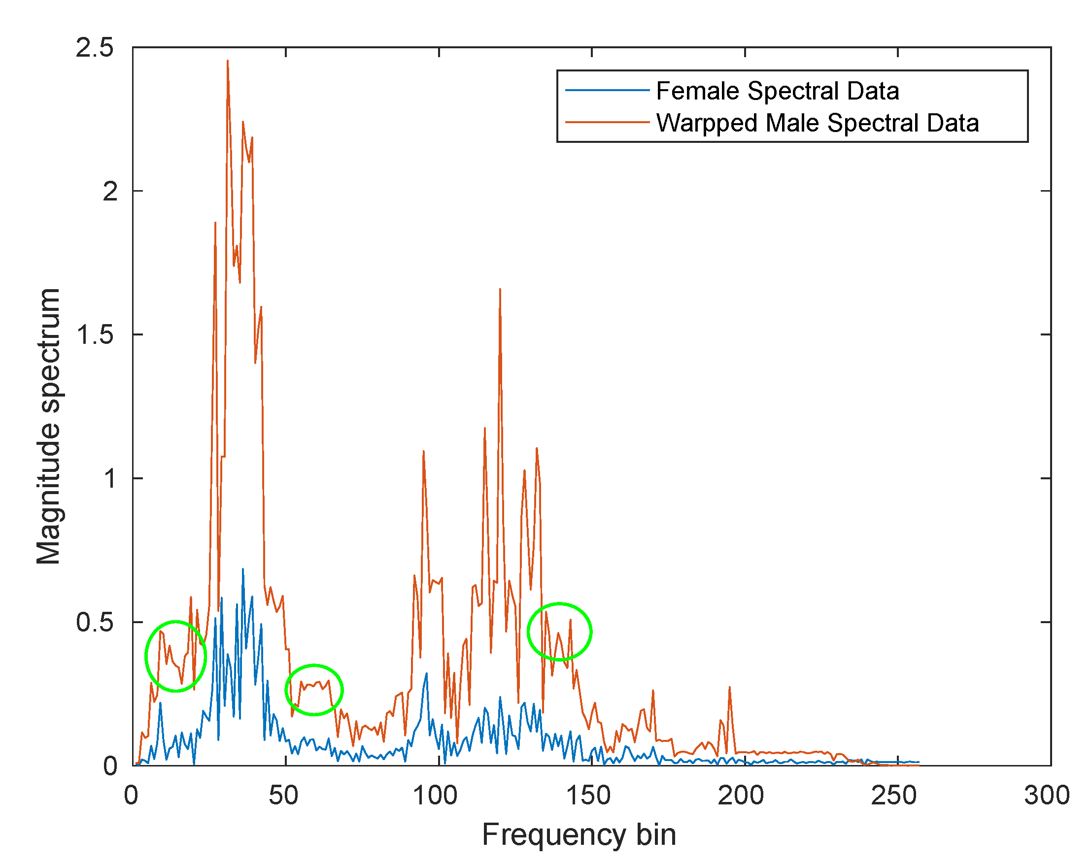
3.2. Experiment Description and a Proof of Concept Result
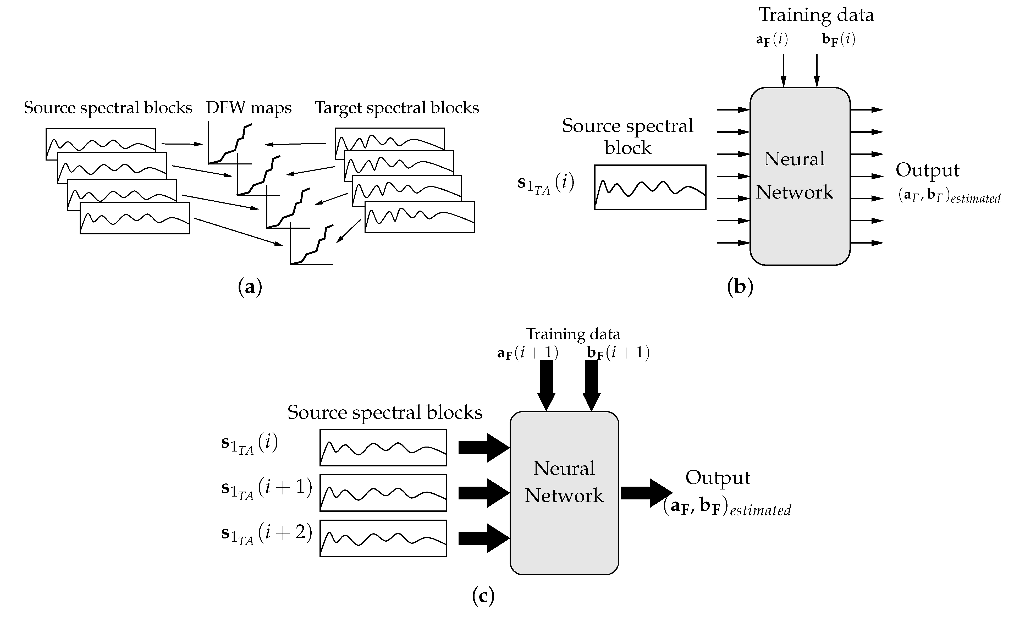
4. Spectral Warping Using NN
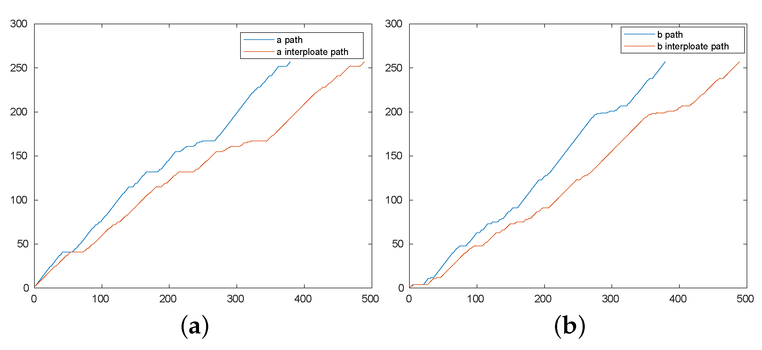
Interpolating the Data to Achieve Constant Length
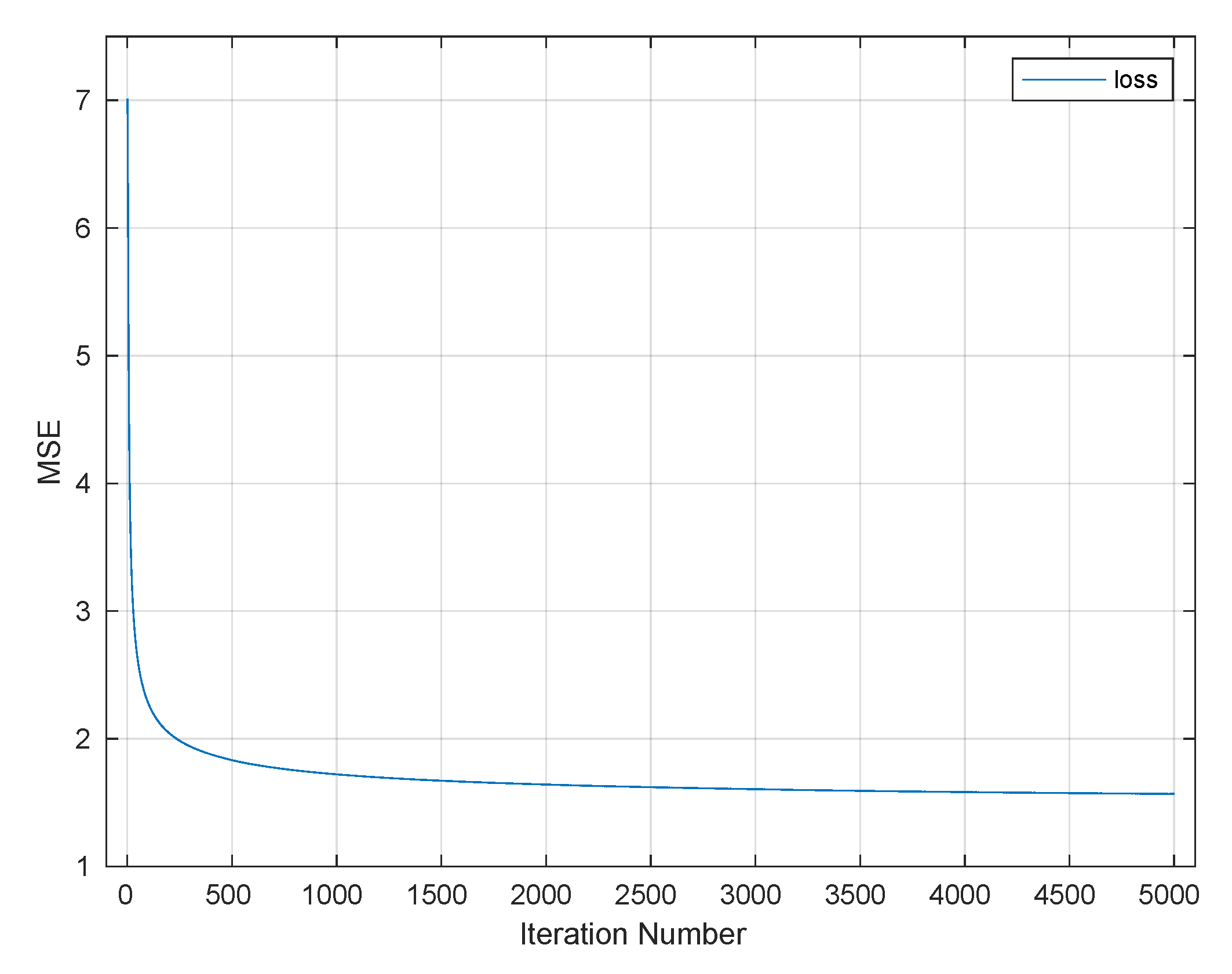
5. Mel-Cepstral Distortion as an Objective Measure
6. NN Architecture Experiments
6.1. Phase One
6.2. Phase Two
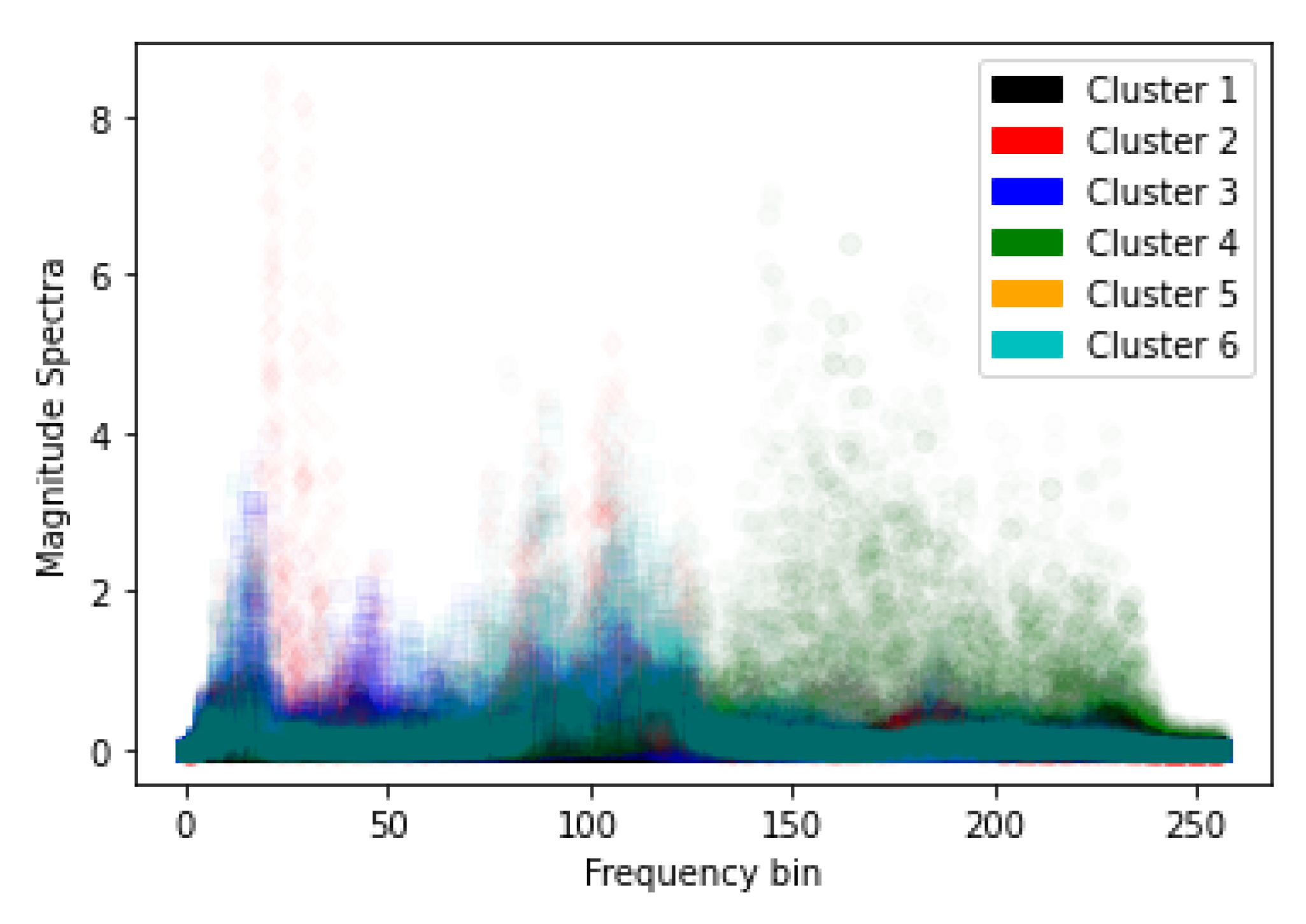
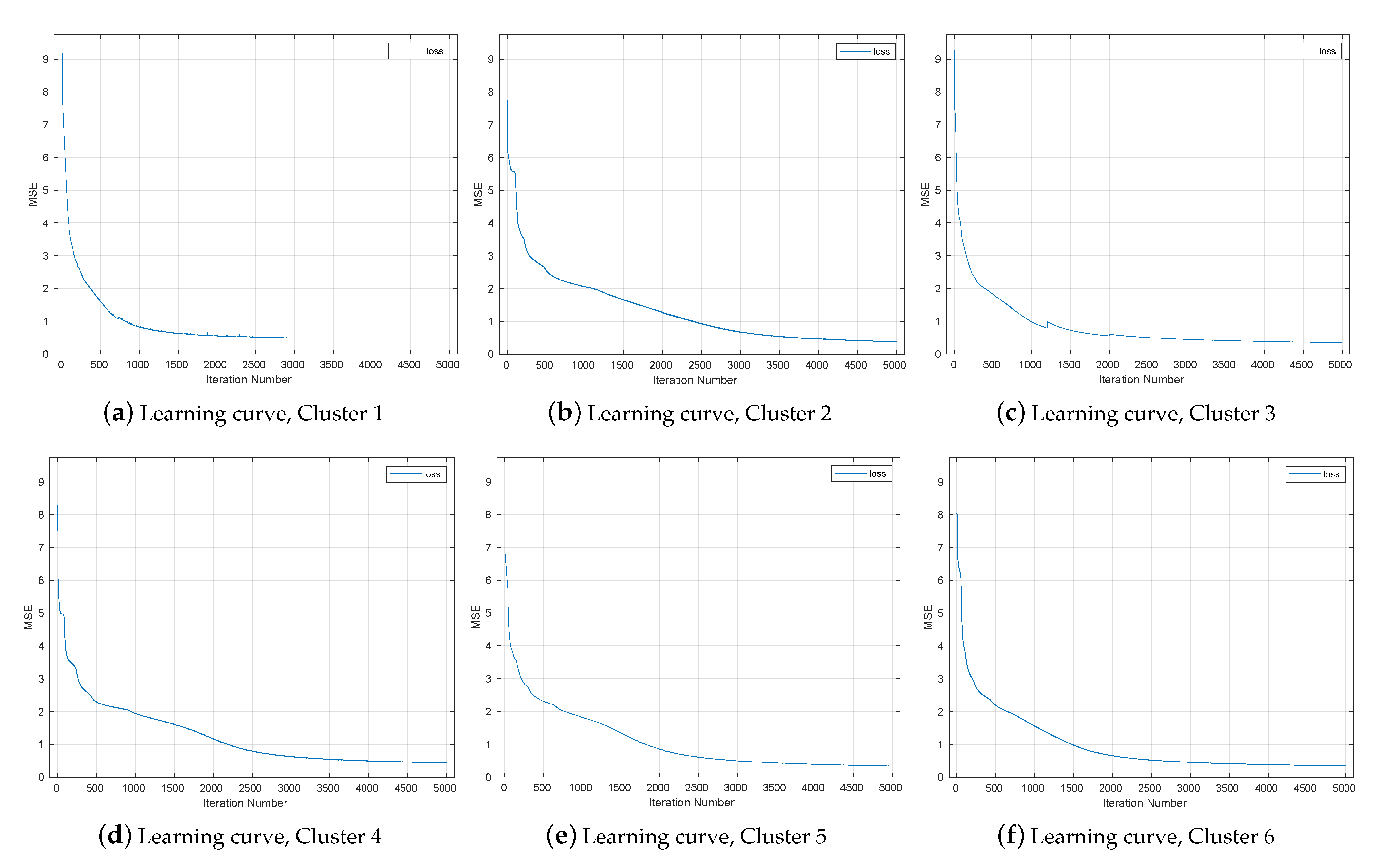
6.3. Phase Three
6.4. Other NN Structures
7. Comparison
8. Summary and Conclusions
Author Contributions
Funding
Institutional Review Board Statement
Informed Consent Statement
Data Availability Statement
Conflicts of Interest
References
- Helander, E.; Schwarz, J.; Nurminen, J.; Silen, H.; Gabbouj, M. On the impact of alignment on voice conversion performance. In Proceedings of the 2008 9th Annual Conference of the International Speech Communication Association, Brisbane, Australia, 22–26 September 2008; Volume 1, pp. 1453–1456. [Google Scholar]
- Narendranath, M.; Murthy, H.A.; Rajendran, S.; Yegnanarayana, B. Transformation of formants for voice conversion using artificial neural networks. Speech Commun. 1995, 16, 207–216. [Google Scholar] [CrossRef] [Green Version]
- Turk, O.; Buyuk, O.; Haznedaroglu, A.; Arslan, L.M. Application of voice conversion for cross-language rap singing transformation. In Proceedings of the IEEE 2009 International Conference on Acoustics, Speech and Signal Processing, (ICASSP), Taipei, Taiwan, 19–24 April 2009; pp. 3597–3600. [Google Scholar]
- Stylianou, Y. Voice transformation: A survey. In Proceedings of the IEEE 2009 International Conference on Acoustics, Speech and Signal Processing (ICASSP), Taipei, Taiwan, 19–24 April 2009; pp. 3585–3588. [Google Scholar]
- Ramos, M.V. Voice Conversion with Deep Learning. Masters of Science Thesis, Universidade do Lisboa, Lisboa, Portugal, 2016. [Google Scholar]
- Abe, M.; Nakamura, S.; Shikano, K.; Kuwabara, H. Voice conversion through vector quantization. J. Acoust. Soc. Jpn. 1990, 11, 71–76. [Google Scholar] [CrossRef] [Green Version]
- Kuwabara, H. Quality control of speech by modifying formant frequencies and bandwidth. In Proceedings of the 11th International Congress of Phonetic Sciences (ICPhS), Tallinn, Estonia, 1–7 August 1987; pp. 281–284. [Google Scholar]
- Childers, D.; Yegnanarayana, B.; Wu, K. Voice conversion: Factors responsible for quality. In Proceedings of the 1985 IEEE International Conference on Acoustics, Speech, and Signal Processing (ICASSP), Tampa, FL, USA, 26 March 1985; Volume 10, pp. 748–751. [Google Scholar]
- Valbret, H.; Moulines, E.; Tubach, J.P. Voice transformation using PSOLA technique. Speech Commun. 1992, 11, 175–187. [Google Scholar] [CrossRef]
- Toth, A.R.; Black, A.W. Using articulatory position data in voice transformation. In Proceedings of the 6th International Speech and Communication Association (ISCA) Workshop on Speech Synthesis, Antwerp, Belgium, 27–31 August 2007; pp. 182–187. [Google Scholar]
- Helander, E.; Virtanen, T.; Nurminen, J.; Gabbouj, M. Voice conversion using partial least squares regression. IEEE Trans. Audio Speech Lang. Process. 2010, 18, 912–921. [Google Scholar] [CrossRef] [Green Version]
- Benisty, H.; Malah, D. Voice conversion using GMM with enhanced global variance. In Proceedings of the 2011 12th Annual Conference of the International Speech Communication Association (ISCA), Florence, Italy, 28–31 August 2011. [Google Scholar]
- Sathiarekha, K.; Kumaresan, S. A survey on the evolution of various voice conversion techniques. In Proceedings of the 2016 IEEE 3rd International Conference on Advanced Computing and Communication Systems (ICACCS), Coimbatore, India, 22–23 January 2016; Volume 1, pp. 1–5. [Google Scholar]
- Yang, Y.; Uchida, H.; Saito, D.; Minematsu, N. Voice Conversion Based on Matrix Variate Gaussian Mixture Model Using Multiple Frame Features. In Proceedings of the 2016 17th Annual Conference of the International Speech Communication Association (ISCA), San Francisco, CA, USA, 8–12 September 2016. [Google Scholar]
- Tian, X.; Lee, S.W.; Wu, Z.; Chng, E.S.; Li, H. An exemplar-based approach to frequency warping for voice conversion. IEEE Trans. Audio Speech Lang. Process. 2017, 25, 1863–1876. [Google Scholar] [CrossRef]
- Sisman, B.; Zhang, M.; Li, H. Group sparse representation with wavenet vocoder adaptation for spectrum and prosody conversion. IEEE Trans. Audio Speech Lang. Process. 2019, 27, 1085–1097. [Google Scholar] [CrossRef]
- Sisman, B.; Yamagishi, J.; King, S.; Li, H. An overview of voice conversion and its challenges: From statistical modeling to deep learning. IEEE Trans. Audio Speech Lang. Process. 2020, 29, 132–157. [Google Scholar] [CrossRef]
- Toda, T.; Black, A.W.; Tokuda, K. Voice conversion based on maximum-likelihood estimation of spectral parameter trajectory. IEEE Trans. Audio Speech Lang. Process. 2007, 15, 2222–2235. [Google Scholar] [CrossRef]
- Zen, H.; Nankaku, Y.; Tokuda, K. Probabilistic feature mapping based on trajectory HMMs. In Proceedings of the 2008 9th Annual Conference of the International Speech Communication Association, Brisbane, Australia, 22–26 September 2008. [Google Scholar]
- Pilkington, N.C.; Zen, H.; Gales, M.J. Gaussian process experts for voice conversion. In Proceedings of the 2011 12th Annual Conference of the International Speech Communication Association, (ISCA), Florence, Italy, 28–31 August 2011. [Google Scholar]
- Xu, N.; Tang, Y.; Bao, J.; Jiang, A.; Liu, X.; Yang, Z. Voice conversion based on Gaussian processes by coherent and asymmetric training with limited training data. Speech Commun. 2014, 58, 124–138. [Google Scholar] [CrossRef]
- Takamichi, S.; Toda, T.; Black, A.W.; Nakamura, S. Modulation spectrum-based post-filter for GMM-based voice conversion. In Proceedings of the IEEE Signal and Information Processing Association Annual Summit and Conference (APSIPA), Chiang Mai, Thailand, 9–12 December 2014; pp. 1–4. [Google Scholar]
- Takamichi, S.; Toda, T.; Black, A.W.; Neubig, G.; Sakti, S.; Nakamura, S. Postfilters to modify the modulation spectrum for statistical parametric speech synthesis. IEEE/ACM Trans. Audio Speech Lang. Process. 2016, 24, 755–767. [Google Scholar] [CrossRef]
- Toda, T.; Muramatsu, T.; Banno, H. Implementation of computationally efficient real-time voice conversion. In Proceedings of the 2012 13th Annual Conference of the International Speech Communication Association, Portland, OR, USA, 9–13 September 2012. [Google Scholar]
- Godoy, E.; Rosec, O.; Chonavel, T. Voice conversion using dynamic frequency warping with amplitude scaling, for parallel or nonparallel corpora. IEEE Trans. Audio Speech Lang. Process. 2012, 20, 1313–1323. [Google Scholar] [CrossRef]
- Mohammadi, S.H.; Kain, A. Transmutative voice conversion. In Proceedings of the 38th 2013 IEEE International Conference on Acoustics, Speech and Signal Processing (ICASSP), Vancouver, BC, Canada, 26–31 May 2013; pp. 6920–6924. [Google Scholar]
- Erro, D.; Navas, E.; Hernaez, I. Parametric voice conversion based on bilinear frequency warping plus amplitude scaling. IEEE Trans. Audio Speech Lang. Process. 2012, 21, 556–566. [Google Scholar] [CrossRef]
- Ayodeji, A.O.; Oyetunji, S.A. Voice conversion using coefficient mapping and neural network. In Proceedings of the 2016 IEEE International Conference for Students on Applied Engineering (ICSAE), Newcastle, UK, 20–21 October 2016; pp. 479–483. [Google Scholar]
- Zhang, M.; Sisman, B.; Zhao, L.; Li, H. Deepconversion: Voice conversion with limited parallel training data. Speech Commun. 2020, 122, 31–43. [Google Scholar] [CrossRef]
- Watanabe, T.; Murakami, T.; Namba, M.; Hoya, T.; Ishida, Y. Transformation of spectral envelope for voice conversion based on radial basis function networks. In Proceedings of the 2002 7th International Conference on Spoken Language Processing, Denver, CO, USA, 16–20 September 2002. [Google Scholar]
- Desai, S.; Raghavendra, E.V.; Yegnanarayana, B.; Black, A.W.; Prahallad, K. Voice conversion using artificial neural networks. In Proceedings of the 2009 IEEE International Conference on Acoustics, Speech and Signal Processing (ICASSP), Taipei, Taiwan, 19–24 April 2009; pp. 3893–3896. [Google Scholar]
- Sun, L.; Kang, S.; Li, K.; Meng, H. Voice conversion using deep bidirectional long short-term memory based recurrent neural networks. In Proceedings of the 2015 IEEE International Conference on Acoustics, Speech and Signal Processing (ICASSP), Brisbane, Australia, 19–24 April 2015; pp. 4869–4873. [Google Scholar]
- Wu, J.; Wu, Z.; Xie, L. On the use of i-vectors and average voice model for voice conversion without parallel data. In Proceedings of the 2016 IEEE Asia-Pacific Signal and Information Processing Association Annual Summit and Conference (APSIPA), Jeju, Korea, 13–16 December 2016; pp. 1–6. [Google Scholar]
- Xie, F.L.; Soong, F.K.; Li, H. A KL Divergence and DNN-Based Approach to Voice Conversion without Parallel Training Sentences. In Proceedings of the 2016 17th Annual Conference of the International Speech Communication Association (ISCA), San Francisco, CA, USA, 8–12 September 2016; pp. 287–291. [Google Scholar]
- Sun, L.; Li, K.; Wang, H.; Kang, S.; Meng, H. Phonetic posteriorgrams for many-to-one voice conversion without parallel data training. In Proceedings of the 2016 IEEE International Conference on Multimedia and Expo (ICME), Seattle, WA, USA, 11–15 July 2016; pp. 1–6. [Google Scholar]
- Sun, L.; Wang, H.; Kang, S.; Li, K.; Meng, H.M. Personalized, Cross-Lingual TTS Using Phonetic Posteriorgrams. In Proceedings of the 2016 17th Annual Conference of the International Speech Communication Association (ISCA), San Francisco, CA, USA, 8–12 September 2016; pp. 322–326. [Google Scholar]
- Hsu, C.C.; Hwang, H.T.; Wu, Y.C.; Tsao, Y.; Wang, H.M. Voice conversion from unaligned corpora using variational autoencoding wasserstein generative adversarial networks. arXiv 2017, arXiv:1704.00849. [Google Scholar]
- Fang, F.; Yamagishi, J.; Echizen, I.; Lorenzo-Trueba, J. High-quality nonparallel voice conversion based on cycle-consistent adversarial network. In Proceedings of the 2018 IEEE International Conference on Acoustics, Speech and Signal Processing (ICASSP), Calgary, AB, Canada, 15–20 April 2018; pp. 5279–5283. [Google Scholar]
- Lorenzo-Trueba, J.; Fang, F.; Wang, X.; Echizen, I.; Yamagishi, J.; Kinnunen, T. Can we steal your vocal identity from the Internet?: Initial investigation of cloning Obama’s voice using GAN, WaveNet and low-quality found data. arXiv 2018, arXiv:1803.00860. [Google Scholar]
- Kameoka, H.; Kaneko, T.; Tanaka, K.; Hojo, N. Stargan-vc: Non-parallel many-to-many voice conversion using star generative adversarial networks. In Proceedings of the 2018 IEEE Spoken Language Technology Workshop (SLT), Athens, Greece, 18–21 December 2018; pp. 266–273. [Google Scholar]
- Parsons, T. Voice and Speech Processing; McGraw Hill: New York, NY, USA, 1987. [Google Scholar]
- Kominek, J.; Black, A.W. The CMU Arctic speech databases. In Proceedings of the 5th International Speech and Communication Association (ISCA) Workshop on Speech Synthesis, Pittsburgh, PA, USA, 14–16 June 2004. [Google Scholar]
- Griffin, D.; Lim, J. Signal estimation from modified short-time Fourier transform. IEEE Trans. Acoust. Speech Signal Process. 1984, 32, 236–243. [Google Scholar] [CrossRef]
- Al-Dulaimi, A.W.; Moon, T.K.; Gunther, J.H. Phase Effects on Speech and Its Influence on Warped Speech. In Proceedings of the 2020 IEEE Intermountain Engineering, Technology and Computing (IETC), Orem, MD, USA, 4–5 May 2020; pp. 1–5. [Google Scholar]


| No. | Two-Level DW Method | MCD [dB] |
|---|---|---|
| 1 | DW, with phase reconstruction | 2.4 |
| 2 | DW, without phase reconstruction | 6.3 |
| Phase No. | Input Model | Architecture Type | NN Architecture | MCD [dB] |
|---|---|---|---|---|
| 5 | 256L 600R 1200R 1000R 964L | 20.5 | ||
| 1-IP-1-OP | 6 | 256L 600R 1000R 1500R 1000R 964L | 18.01 | |
| 7 | 256L 600R 1000R 1500R 2000R 1500R 964L | 18.002 | ||
| 19 | 500L 1500R 2500R 3500R 4500R 5040R 6459R 7459R | 3.3 | ||
| 8459R 9459R 10459R 8459R 7939R 6939R 5500R 4500R | ||||
| 3500R 2500R 964L | ||||
| Phase One | 20 | 500L 1500R 2500R 3500R 4500R 5040R 6459R 7459R | 5.5 | |
| 8459R 9459R 10459R 9459R 8459R 7939R 6939R 5500R | ||||
| 4500R 3500R 2500R 964L | ||||
| 5 | 768L 4500R 6500R 6939R 964L | 16.85 | ||
| 6 | 768L 4500R 6500R 7040R 6939R 964L | 15.3 | ||
| 3-IP-1-OP | 7 | 768L 4500R 6500R 8040R 8939R 6939R 964L | 12.92 | |
| 9 | 768L 4500R 6500R 7040R 9459R 8939R 7939R 6939R 964L | 7.5 | ||
| 10 | 768L 4500R 6500R 7040R 9459R 10459R 8939R 7939R 6939R 964L | 4.7 | ||
| 19 | 1500L 2500R 3500R 4500R 6500R 7040R 8459R | 2.25 | ||
| 9459R 10459R 10459R 9459R 8459R 7939R 6939R 5500R 4500R | ||||
| 3500R 2500R 964L | ||||
| 20 | 1500L 2500R 3500R 4500R 6500R 7040R 8459R 9459R | 3.5 | ||
| 10459R 11459R 10459R 9459R 8459R 7939R 6939R 5500R 4500R | ||||
| 3500R 2500R 964L | ||||
| Phase Two | 3-IP-1-OP | 19 | 1500L 2500R 3500R 4500R 6500R 7040R 8459R 9459R | 4.8 |
| 10459R 9459R 8459R 7939R 6939R 5500R 4500R 3500R | ||||
| 2500R 964L | ||||
| Phase Three | 3-IP-1-OP | Six-Clusters.Each Cluster trained for 19 layers | 1500L 2500R 3500R 4500R 6500R 7040R 8459R 9459R 10459R | 2.8 |
| 10459R 9459R 8459R 7939R 6939R 5500R 4500R 3500R 2500R | ||||
| 964L | ||||
| Phase Four | 1-IP-1-OP | 7 | 256L 64R (k = 3) 100R (k = 3) 150R (k = 3) 100R (k = 3) FL D100R 964L | 13.33 |
| 3-IP-1-OP | 5 | 768L 64R (k = 3) 100R (k = 3) FL D100R 964L | 13.5 |
Publisher’s Note: MDPI stays neutral with regard to jurisdictional claims in published maps and institutional affiliations. |
© 2021 by the authors. Licensee MDPI, Basel, Switzerland. This article is an open access article distributed under the terms and conditions of the Creative Commons Attribution (CC BY) license (https://creativecommons.org/licenses/by/4.0/).
Share and Cite
Al-Dulaimi, A.-W.; Moon, T.K.; Gunther, J.H. Voice Transformation Using Two-Level Dynamic Warping and Neural Networks. Signals 2021, 2, 456-474. https://doi.org/10.3390/signals2030028
Al-Dulaimi A-W, Moon TK, Gunther JH. Voice Transformation Using Two-Level Dynamic Warping and Neural Networks. Signals. 2021; 2(3):456-474. https://doi.org/10.3390/signals2030028
Chicago/Turabian StyleAl-Dulaimi, Al-Waled, Todd K. Moon, and Jacob H. Gunther. 2021. "Voice Transformation Using Two-Level Dynamic Warping and Neural Networks" Signals 2, no. 3: 456-474. https://doi.org/10.3390/signals2030028
APA StyleAl-Dulaimi, A.-W., Moon, T. K., & Gunther, J. H. (2021). Voice Transformation Using Two-Level Dynamic Warping and Neural Networks. Signals, 2(3), 456-474. https://doi.org/10.3390/signals2030028