Real-Time Analysis of Millidecade Spectra for Ocean Sound Identification and Wind Speed Quantification

Abstract

This study introduces an algorithm for quantifying oceanic wind speed and identifying sound sources in the local underwater soundscape. Utilizing low-complexity metrics like one-minute spectral kurtosis and power spectral density levels, the algorithm categorizes different soundscapes and estimates wind speed. It detects rain, vessels, fin and blue whales, as well as clicks and whistles from dolphins. Positioned as a foundational tool for implementing the Ocean Sound Essential Ocean Variable (EOV), it contributes to understanding long-term trends in climate change for sustainable ocean health and predicting threats through forecasts. The proposed soundscape classification algorithm, validated using extensive acoustic recordings (≥32 kHz) collected at various depths and latitudes, demonstrates high performance, achieving an average precision of $89\%$ and an average recall of $86.59\%$ through optimized parameter tuning via a genetic algorithm. Here, wind speed is determined using a cubic function with power spectral density (PSD) at 6 kHz and the MASLUW method, exhibiting strong agreement with satellite data below 15 m/s. Designed for compatibility with low-power electronics, the algorithm can be applied to both archival datasets and real-time data streams. It provides a straightforward metric for ocean monitoring and sound source identification.

1. Introduction

In 2018, the Global Ocean Observing System (GOOS) formally introduced Ocean Sound as a cross-disciplinary Essential Ocean Variable (EOV) [1], which officially recognized sound’s role as a parameter for assessing ecosystem health, climate change, and human impact on the ocean [2]. Ocean sound is inherently multidisciplinary, as it can be analyzed to assess physical parameters like wind speed [3,4,5], rain rate [6,7], and sea-ice presence [8] and detect the presence of sound-producing animals including marine mammals, many fish, some invertebrates [9] and sounds from human activities. Human sounds such as shipping noise [10,11], seismic airgun surveys, sonars, and pile driving are known to injure and disturb marine life of all taxa [12,13,14] as well as mask the sounds animals use for communication, socialization, foraging, and navigation [15,16]. Thus, tracking the contribution of human sounds to ecosystems around the globe is an indicator of the acoustic quality of an ecosystem for the animals. For example, the quantity and quality of sound on shallow water coral reefs is correlated with the health of those reefs [17,18,19].

The Ocean Sound EOV was established to provide a framework for detecting and interpreting ecosystem changes. It facilitates this by comparing acoustic metrics in various periods and geographical contexts. Specifically, a systematic analysis of soundscape variations allows researchers to track changes in biodiversity, ecosystem health, and overall ecological balance [20]. By tracking the dynamics of marine environments, the global community will develop the ability to predict future changes, contributing to informed conservation and management strategies. This EOV will offer valuable information on the scale and impacts of anthropogenic activity by analyzing global Ocean Sound data over extended periods [21]. This knowledge will guide us in creating sustainable practices and policies, thus promoting the harmony between human activities and marine life.

Changes in human activity during the COVID-19 pandemic highlight how systematic Ocean Sound reporting enables the community to measure environmental changes.Although a systematic EOV is not yet in place, several groups have studied changes in marine acoustic environments during lockdowns and restrictions, revealing the direct impact of reduced human activity on underwater soundscapes [22]. The measures enacted to mitigate the COVID-19 pandemic led to significant changes in human activity, resulting in a prolonged reduction in seismic noise. The seismic noise quiet period experienced in 2020 stands as a notable global anthropogenic seismic noise reduction on record [23,24]. In addition, measurements of power spectral density (PSD) at 100 Hz in the Port of Vancouver indicated a decline in shipping activity during the COVID-19 pandemic [25]. It was also observed that the investigation of changes in the acoustic environment due to COVID-19 was hampered by a lack of accessible and standardized data products from around the globe [26,27].

In 2023, the Ocean Sound EOV Implementation Plan [28] was published. It documents the role of Ocean Sound in supporting the GOOS core mandates of measuring climate change and ocean health and monitoring threats. The plan identifies 11 tasks to fully implement the EOV, which are divided into four broad groups: (1) maintaining the existing Ocean Sound measurement sites and gathering essential oceanic data; (2) developing standardized metrics to report Ocean Sound; (3) funding openly accessible databases to host and distribute Ocean Sound data; and (4) developing hindcast, nowcast, and forecast Ocean Sound models. Numerous international workshops have been held to establish a minimum set of soundscape metrics [29,30]. These have been demonstrated and further refined in large-scale monitoring projects [31,32] and are now being formalized in the first revision of the ISO Standard 7605 (Underwater acoustics—Measurement of underwater ambient sound standard) [33] for the measurement and reporting of ambient sound. These initial recommendations focus on documenting the sound pressure levels in time and frequency by reporting, as a minimum, the one-minute decidecade and decade sound pressure levels. In general, it is also recommended to report the per-second values to increase the temporal resolution and hybrid millidecade values [34] to increase the frequency resolution.

Currently, there are no standardized methods for measuring wind speed, rain, or human and biological contributions to the soundscape. The works of [3,4] provide a means of quantifying wind and rain rates; however, they are presented as appropriate for specific environments (the Mediterranean Sea and the Greek Sea, respectively). Based on the successful quantification of the diversity of species in the air, attempts have been made to employ metrics such as entropy, diversity, and complexity to describe the underwater soundscape [35,36,37]. However, these have been unsuccessful because of the long underwater acoustic propagation ranges, as well as the temporal and frequency overlap between human, natural, and biological sound sources. However, some metrics have shown the ability to distinguish between soundscapes [38]. However, detecting individual sound sources using various detectors has proven more effective than relying on general-purpose metrics for underwater soundscapes [39,40,41].

An effective algorithm for oceanic data analysis must meet several key requirements to ensure its utility. Oceanic data analysis involves processing and interpreting various environmental and biological signals collected from the ocean to monitor weather patterns, assess marine biodiversity, and evaluate human impacts on underwater ecosystems. One critical aspect of this analysis is the ability to assess atmospheric conditions. For example, accurately estimating wind speed and detecting the presence of rain can provide valuable in situ measurements that contribute to weather forecasting and storm mitigation [42]. Oceanic gliders and drifters (e.g., ARGOS floats) can enhance meteorological models and improve disaster preparedness if these data are transmitted in near-real-time.

Beyond environmental factors, the algorithm should facilitate biological monitoring by identifying sentinel species, such as fin and blue whales, and recognizing delphinid clicks and whistles. In addition, it should be capable of detecting human-induced sound sources, particularly vessels, to provide information on anthropogenic impacts on the underwater environment. To ensure data reliability, the algorithm must also recognize and account for flow noise as part of a quality assurance process. The reliability of the algorithm is crucial; It should maintain high accuracy in detecting and estimating environmental and biological parameters across various water depths and latitudes, ensuring its applicability in various oceanic environments. Finally, to improve practicality and accessibility, the algorithm must be compatible with low-power embedded systems, allowing efficient computation in resource-constrained environments [43].

An algorithm was introduced by Nystuen et al. [4] to measure the wind speed and classify sources in underwater soundscapes. In their algorithm, shipping and odontocete echolocation sound sources are detected; then those samples are excluded, and rainfall categories are established. Finally, the wind speed was measured using the third-order polynomial of the PSD at 8 kHz.

This paper proposes an algorithm that extends the work of Nystuen et al. [4] and can serve as an easily accessible means of detecting sound sources for the Ocean Sound EOV. Regarding physical ocean parameters, the algorithm estimates the wind speed and the type of rain that occurs. Concerning biological sound sources, it detects the presence of fin and blue whale choruses as well as odontocete clicks and whistles. The algorithm also detects the presence of shipping activities as an indicator of human activity.

In this study, analyses were performed on 19 different datasets, totaling 1,016,890 min of data, stored in the form of millisecond millidiameter spectral data. An empirical algorithm was developed, based on [4], to analyze each one-minute millidecade spectrum to identify rain, vessels, fin and blue whales, and odontocete clicks and whistles. The algorithm first identified sound sources, which were then validated using an automated data selection and validation algorithm [44]. This algorithm selected 100 min from each dataset for the manual verification of the detected sound sources. The classifier was then refined through the application of the Genetic Optimization algorithm.

After the classification process, the wind speed is calculated using a cubic function of PSD at 6 kHz based on the recording depth. The resulting wind speed estimation shows good agreement with satellite data, particularly for speeds below 15 m/s, and maintains a low complexity suitable for embedding on remote nodes.

The subsequent sections of this paper are organized as follows: Section 2 describes the datasets employed. Section 3 presents an overview of the dataset pre-processing, including the depth correction process for the sound pressure level. In Section 4, the classification algorithm is explained, and its performance is documented. Section 5 describes the quantification of the wind speed rate and compares the estimates to wind speeds derived from hindcast models. Finally, Section 6 provides the conclusion.

2. Data Collection

The one-minute acoustic data utilized in this paper were collected between March 2013 and October 2021 using autonomous multichannel acoustic recorders (AMARs) with a nominal sensitivity of $-164 \mathrm{dB} \mathrm{V}/\mathsf{\mu }\mathrm{Pa}$, manufactured by JASCO Applied Science Ltd. The AMARs utilize hydrophones from GeoSpectrum Technologies Inc. (Dartmouth, NS, Canada). The recordings encompass various water depths and a broad range of latitudes, with all data sampled at 32 kHz or higher. For all recordings used in the wind speed analysis, the system noise floor at 6 kHz was $35\mathrm{dB}\mathrm{re}1\mathsf{\mu }{\mathrm{Pa}}^2/\mathrm{Hz}$ or lower.

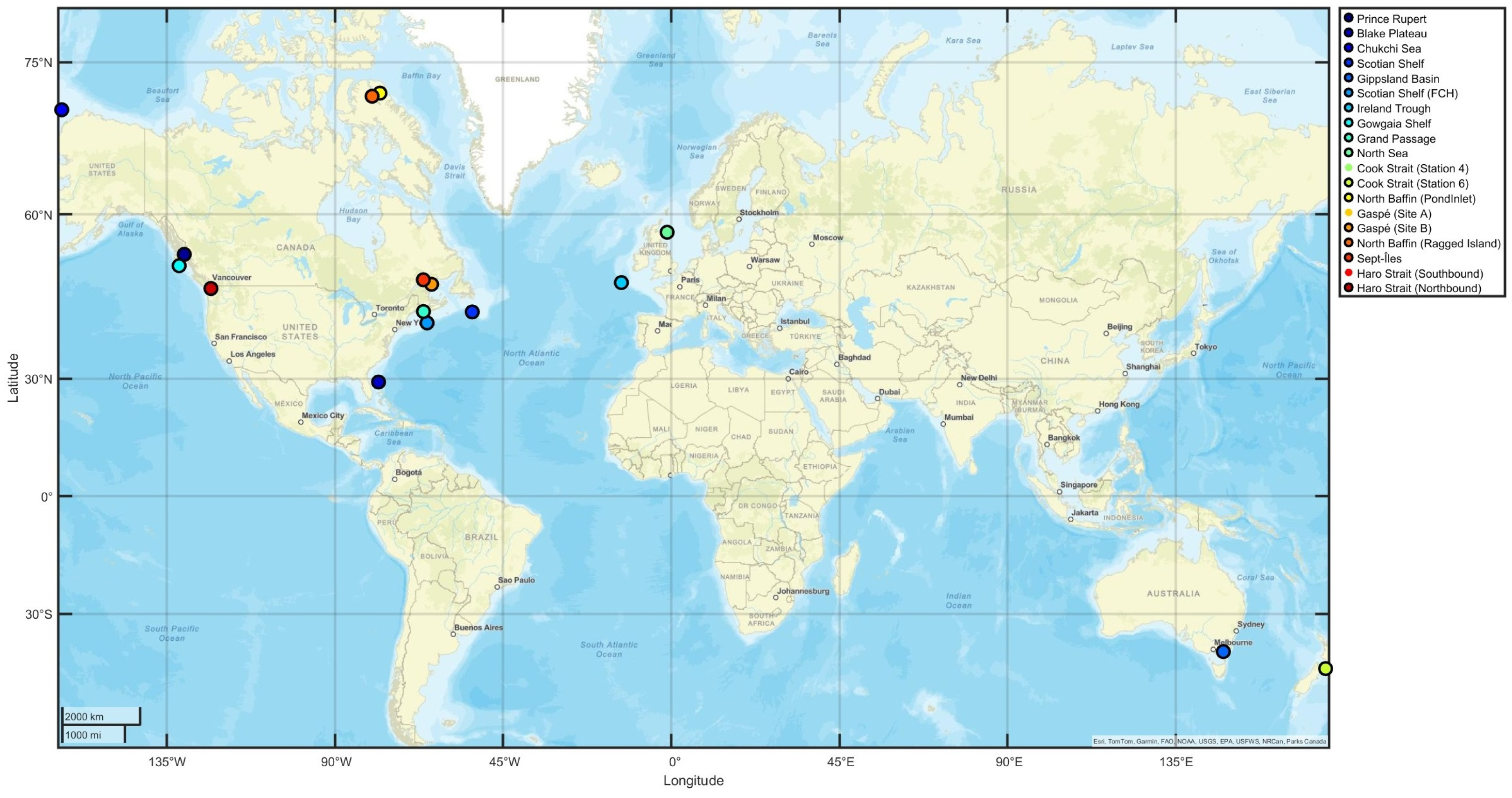
The data locations are shown in Figure 1.

Table 1. Deployment information for various oceanic stations.

Location Name of the Station	Duration of Deployment	Depth (m)	Sampling Rate (Hz)	Number of Minutes	Latitude	Longitude
Prince Rupert	22 March 2013 to 25 September 2013	80	64,000	62,755	54.2087°	−130.34087°
Blake Plateau	6 November 2018 to 16 November 2019	900	512,000	54,020	29.2506°	−78.35106667°
Chukchi Sea *	5 August 2014 to 14 October 2014	50	375,000	13,400	$71.{33516667}^{°}$	$-163.{1243667}^{°}$
Scotian Shelf *	17 July 2016 to 19 July 2017	1547	250,000	26,422	$44.{19273333}^{°}$	$-53.{27476667}^{°}$
Gippsland Basin	26 March 2021 to 13 April 2021	75	128,000	25,370	$-38.{326275}^{°}$	$147.{7111}^{°}$
Scotian Shelf (FCH)	8 October 2019 to 2 September 2020	1452	256,000	190,146	$42.{041}^{°}$	$-65.{3622}^{°}$
Ireland Trough *	19 March 2016 to 9 August 2016	1750	250,000	28,540	$49.{54771}^{°}$	$-13.{37298}^{°}$
Gowgaia Shelf *	25 July 2019 to 25 July 2020	744	250,000	35,130	$52.{39333333}^{°}$	−131.7137°
Grand Passage	14 October 2020 to 12 November 2020	43	512,000	8157	$44.{269182}^{°}$	$-66.{339397}^{°}$
North Sea	21 October 2020 to 24 January 2021	100	64,000	136,861	$57.{530018}^{°}$	$-1.{1263334}^{°}$
Cook Strait (Station 4) *	28 April 2016 to 20 December 2016	1022	250,000	37,680	$-41.{61233}^{°}$	$174.{7353}^{°}$
Cook Strait (Station 6) *	28 April 2016 to 21 December 2016	1486	250,000	38,154	$-41.{805017}^{°}$	$175.{081}^{°}$
North Baffin (PondInlet)	8 August 2021 to 14 September 2021	131	64,000	50,386	$72.{70773}^{°}$	$-77.{98278}^{°}$
Gaspé (Site A)	4 September 2019 to 30 October 2019	335	128,000	80,530	$49.{1042}^{°}$	$-64.{28408333}^{°}$
Gaspé (Site B)	4 September 2019 to 30 October 2019	384	128,000	80,540	$49.{25856667}^{°}$	$-64.{1588}^{°}$
North Baffin (Ragged Island)	2 August 2021 to 13 September 2021	130	512,000	4047	$72.{46352}^{°}$	$-80.{07005}^{°}$
Sept-Îles	26 March 2021 to 13 April 2021	85	32,000	102,522	$50.{03606}^{°}$	$-66.{36876}^{°}$
Haro Strait (Southbound)	26 March 2021 to 13 April 2021	250	128,000	8640	$48.{51811667}^{°}$	$-123.{1915833}^{°}$
Haro Strait (Northbound)	26 March 2021 to 13 April 2021	205	128,000	8640	$48.{51646667}^{°}$	$-123.{2076667}^{°}$

The data indicated by * were not used for estimating the wind speed.

details the location, deployment duration, water depth, sample rates, and total minutes of acoustic data collected for each dataset.

Wind speed information incorporated in this study is derived from the ERA5 dataset for meteorological data. ERA5, a global atmospheric reanalysis tool developed by the European Center for Medium-Range Weather Forecasts (ECMWF), provides a detailed and high-resolution representation of historical weather conditions [45]. Wind speed data are retrieved from the Copernicus Climate Change Service (C3S) web service, serving as an accessible interface for ERA5 data [46].

The Grand Passage (Nova Scotia, Canada) dataset was measured in an area with high currents. The current speeds in this area were obtained using an acoustic doppler current profiler (ADCP). For this purpose, the current data is instrumental in enabling the analysis of flow noise. To support the analysis of shipping detection, automatic identification system (AIS) data near the Gaspé stations [47] was obtained for the corresponding acoustic recordings from September to October 2019.

Figure 2 shows the process of analyzing millidecade PSD data. Initially, the raw PSD data undergo offset correction. After correction, the data are fed into two distinct algorithms. One algorithm estimates the wind speed, while the other classifies the soundscape into different sources.

3. The Offset Correction Process

Underwater ambient noise measurements are influenced by various factors, such as source directionality, spreading losses, attenuation, refraction, and multipath propagation, all of which vary with frequency. To ensure reliable and comparable measurements, the PSD must be standardized for depth and seawater absorption. In an isovelocity sound speed profile—where sound speed remains constant with depth—a correction factor compensates for signal loss due to absorption and path geometry. Higher frequencies require more correction because they experience greater absorption and spreading losses. The absorption coefficient is calculated using Ainslie and McColm’s model [48]. This correction improves the robustness of PSD measurement, adapting it to varying environmental conditions such as depth, salinity, and temperature. This method is particularly valuable for estimating oceanic wind speed and analyzing other underwater acoustic phenomena.

4. The Classifier Algorithm

An optimized algorithm was designed to classify a broad range of underwater acoustic signatures. Each one-minute segment, formatted in hybrid millidecades of recorded underwater acoustics, undergoes processing to determine its class and soundscape type. Adopting hybrid millidecade-formatted data proves to be an effective solution to significantly reduce the size of the spectral data. The hybrid format utilizes a 1 Hz resolution up to 435 Hz and millidecade frequency bands beyond 435 Hz. Millidecades represent logarithmically spaced frequency bands with a bandwidth equivalent to 1/1000 th of a decade [34].

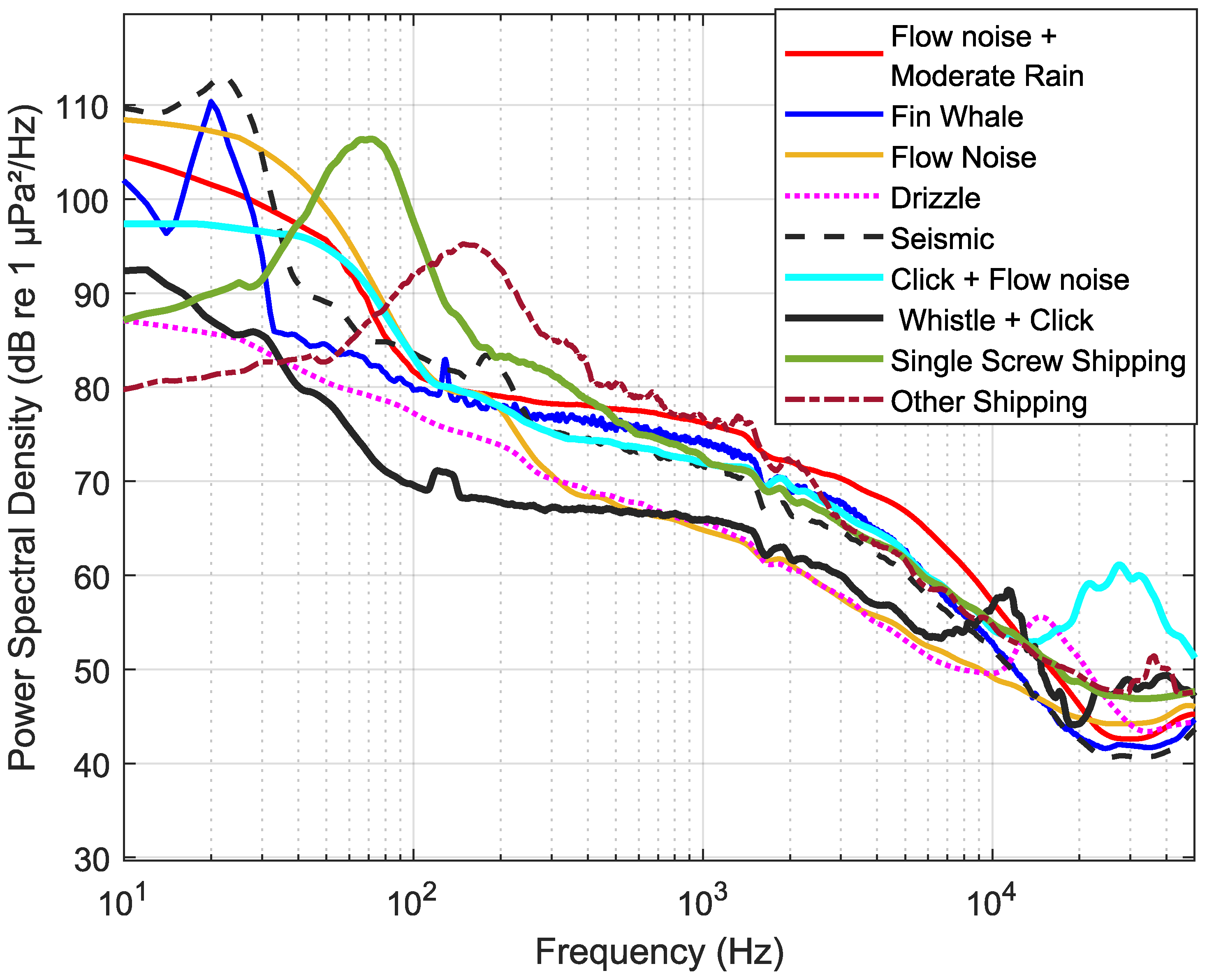
Figure 3 shows an example of the classification of different acoustic sources. This classification was validated through automated and manual analyses, which will be explained in further detail.

As evident in the examples presented in Figure 3, the PSD for flow noise shows a prominent increase at frequencies below 30 Hz, surpassing $75\mathrm{dB}\mathrm{re}1\mathsf{\mu }{\mathrm{Pa}}^2/\mathrm{Hz}$. A shallow slope in frequencies between 2 kHz to 6 kHz is observed in the PSD for moderate rain. Also, the PSD level within this frequency range exceeds $70\mathrm{dB}\mathrm{re}1\mathsf{\mu }{\mathrm{Pa}}^2/\mathrm{Hz}$. The distinctive features of the PSD include a sharp peak at a high frequency of 30 kHz, indicative of dolphin clicks, and a peak at 10 kHz, representing dolphin whistles. Identifying seismic activity requires both temporal and spectral analyses, with discernible peaks in the PSD occurring in the frequency range of 20 to 120 Hz.

The presence of heavy shipping (single-screw vessels) is characterized by a PSD peak around 50 Hz, while light shipping exhibits a peak around 200 Hz, with PSD levels exceeding $80\mathrm{dB}\mathrm{re}1\mathsf{\mu }{\mathrm{Pa}}^2/\mathrm{Hz}$ for any shipping activities. The presence of fin whales is discernible by a peak at 20 Hz.

Section 4.1 provides an overview of key acoustic characteristics crucial for the proposed classification of underwater soundscapes. Following this, the classification approach is described in Section 4.2. The process of manual data analysis is explained in Section 4.3. Subsequently, Section 4.4 introduces the proposed classification algorithm. Finally, the classifier’s performance is documented in Section 4.5.

4.1. Feature Extraction and Employed Metrics

The proposed algorithm classifies underwater soundscapes by identifying discriminative features in the frequency spectrum.

Spectral features play a vital role in revealing the energy distribution across diverse frequencies, with PSD standing out as the most important metric in this domain. PSD provides valuable insights into how power or energy is distributed across the various frequency components of a signal. Distinctive patterns can be identified through the analysis of PSD, including the presence of harmonics, peaks, or specific frequency bands associated with unique characteristics of underwater acoustics.

Spectral kurtosis is a statistical metric that quantifies the sharpness of peaks in the frequency spectrum. It is mathematically represented by ${\beta }_f$ and is calculated using

$$\begin{array}{c}\hfill {\beta }_f={\displaystyle \frac{1/N_f{\sum }_f{(PSD\left(f\right)-\overline{PSD})}^4}{{{\sigma }_f}^2}},\end{array}$$

(1)

where $N_f$ is the number of points for the fast Fourier transform (FFT), $PSD\left(f\right)$ represents the PSD value at frequency f, $\overline{PSD}$ is the mean of the PSD, and ${\sigma }_f$ is the standard deviation of the PSD. Kurtosis [49] theoretically spans an unbounded range. However, practical interpretation commonly focuses on values around 3. A kurtosis of 3 indicates a mesokurtic distribution, the standard or normal level. Values greater than 3 indicate leptokurtic distributions with heavier tails and a more peaked shape (impulsive or tonal features, e.g., dolphin clicks). In contrast, values less than 3 suggest platykurtic distributions characterized by lighter tails and a flatter shape (uniformly distributed spectral content).

The slope of the spectrum serves various purposes within the algorithm. Meanwhile, the coefficient of determination ($R^2$) is employed to assess the goodness of fit of a linear regression model, ensuring that the data accurately represent the parameter being characterized. $R^2$ is calculated using

$$\begin{array}{cc}\hfill R^2& =1-{\displaystyle \frac{{\sum }_{i=1}^n{({\mathrm{PSD}}_i-{\widehat{PSD}}_i)}^2}{{\sum }_{i=1}^n{({PSD}_i-\overline{PSD})}^2}}\hfill \end{array}$$

(2)

where ${PSD}_i$ represents the observed power spectral density at frequency i, $\overline{PSD}$ denotes the mean power spectral density, and ${\widehat{PSD}}_i$ signifies the predicted power spectral density at frequency i. Also, n is the number of frequencies.

4.2. Optimized Classification Algorithm

The presented classification algorithm introduces an optimization approach by fine-tuning parameters that serve as thresholds for key features in the classification process, such as the kurtosis threshold, the R-squared range ($R^2$), the slope range, the frequency range (either singular or multiple), and the PSD threshold for a specified frequency range. These thresholds are dynamically optimized using a genetic algorithm (GA) to achieve the best possible classification performance [50].

The algorithm commences with the initialization of these parameters, and the 1-min millidecade data undergoes offset correction as specified in Section 3. The subsequent step involves feature extraction, specifically focusing on temporal and spectral characteristics like kurtosis, regression features, and the mean PSD, as detailed for each source in later sections.

The iterative optimization process shown in Figure 4 begins, guided by the genetic algorithm, which systematically refines the thresholds ($a,b,c,d,$ …) by comparing the model predictions with known truth data (see Section 4.3) to enhance the performance of the classification model. The genetic algorithm generates a population of potential threshold configurations and evaluates them using the F1 score, which balances precision and recall in binary classification tasks. The GA then selects solutions for reproduction, performs crossover to exchange genetic material, introduces variations through mutations, and updates the population with new offsprings [51,52,53]. The termination condition is met when the cost function, derived from the F1 score, falls below a predefined threshold, indicating satisfactory classification performance.

It is important to note that the initial population of threshold values was seeded using an expert-based approach. Specifically, the threshold ranges were informed by prior domain knowledge and preliminary analyses of characteristic spectral features associated with various sound sources. The algorithm’s modular design allows easy adaptation to different datasets and requirements. Integrating pre-processing, feature extraction, classification, and parameter optimization in a unified framework provides an effective solution for tailored classification optimization.

The Algorithm 1 outlines the steps of the proposed optimized classification process. Detailed explanations of the truth dataset and the automated classifier will follow in subsequent sections.

Algorithm 1 Optimized Classification Algorithm

1: function PreprocessData(Raw Data) 2:       Implement offset correction algorithm 3:       return Pre-processed Data 4: end function 5: function ExtractFeatures($a,b,c,d$, Pre-processed Data) 6:       Implement feature extraction algorithm 7:       return Features 8: end function 9: function RunClassifier(Features) 10:       Implement classifier algorithm 11:       return Predictions 12: end function 13: function CalculateF1Score(Predictions, Truth Data) 14:       Implement F1 score calculation logic 15:       return F1_Score 16: end function 17: function CostFunction(F1_Score) 18:       $F_{\mathrm{opt}}\leftarrow 1-\mathrm{F1\_Score}$ 19:       return $F_{\mathrm{opt}}$ 20: end function 21: function OptimizeParameters($a,b,c,d,F_{\mathrm{opt}}$) 22:       $[\mathrm{output},\mathrm{population},\mathrm{scores}]\leftarrow \mathrm{ga}(F_{\mathrm{opt}},N,lb,ub,options)$ 23:       Update parameters based on optimization strategy 24:       return $a_{\mathrm{new}},b_{\mathrm{new}},c_{\mathrm{new}},d_{\mathrm{new}}$ 25: end function 26: procedure  Main 27:       Raw Data ← Load Raw Data 28:       Pre-processed Data ← PreprocessData(Raw Data) 29:       $a,b,c,d\leftarrow$ InitialParameters() 30:       while True do 31:           Features ←ExtractFeatures($a,b,c,d$, Pre-processed Data) 32:           Predictions ← RunClassifier(Features) 33:           F1_Score ← CalculateF1Score(Predictions, Truth Data) 34:           $F_{\mathrm{opt}}\leftarrow$ CostFunction(F1_Score) 35:           if $F_{\mathrm{opt}}<$ threshold then 36:                break 37:           end if 38:           $a,b,c,d\leftarrow$OptimizeParameters($a,b,c,d,F_{\mathrm{opt}}$) 39:       end while 40: end procedure

4.3. Manual Data Analysis

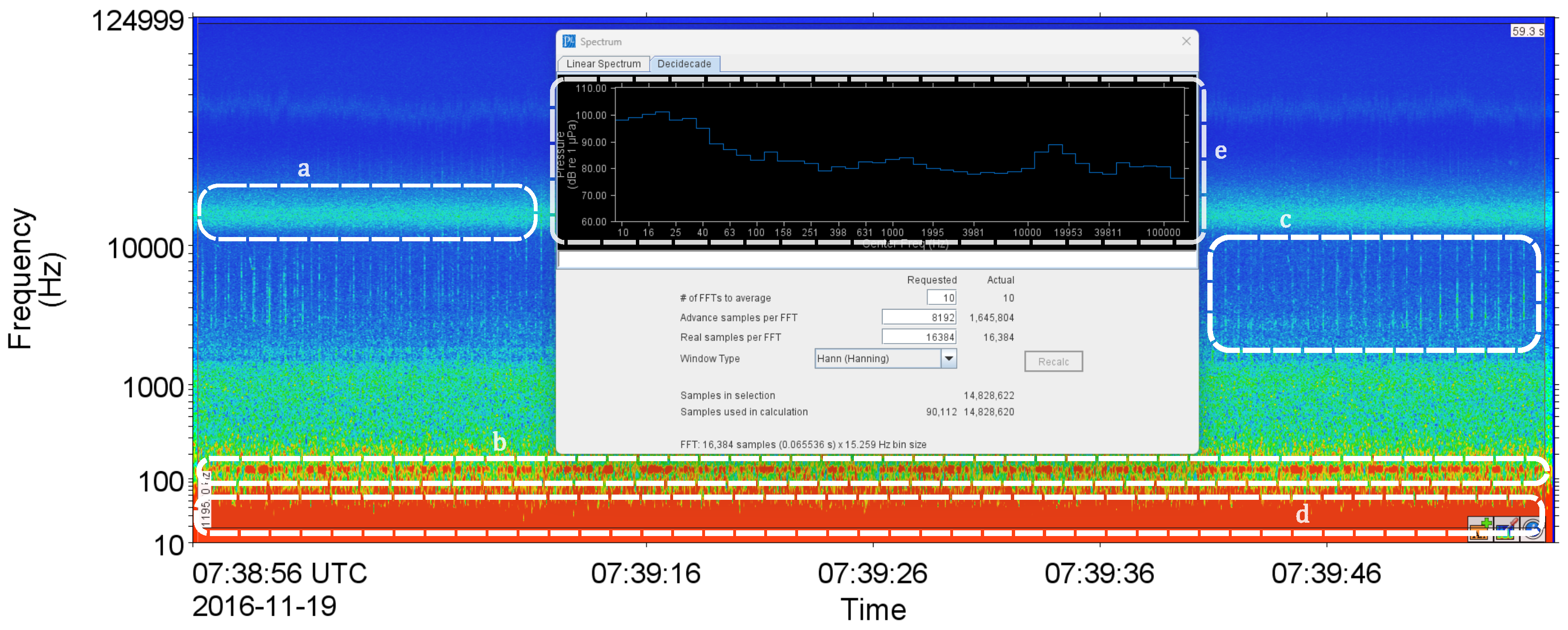
To assess the classifier’s performance, a rigorous manual analysis was undertaken to establish a broad truth dataset that includes a diverse set of acoustic events amid local noise. Using the automated data selection for validation (ADSV) algorithm [44], a carefully curated subset of one-minute acoustic files was selected from the dataset shown in Table 1. These files were chosen to represent the detailed acoustic conditions within the dataset, allowing for manual review and validation. Trained analysts examined these files using PAMlab (JASCO Applied Sciences’tool). The analyst annotated each file, discerning the presence or absence of each source in the annotation sets based on the time and frequency behavior of the acoustic signal. The annotations for each one-minute file may encompass fin whales, blue whales, delphinid clicks and whistles, seismic activity, light shipping, heavy shipping, light rain, moderate rain, heavy rain, and flow noise. Within PAMLab, the analysts employ specific functionalities for file annotation, utilizing tools such as the average power spectral density (Box (e) in Figure 4) and a spectrogram with user-defined FFT settings. Figure 4 shows a spectrogram of a recorded file sampled on a one-minute interval. The data is from the Scotian Shelf and was recorded for the Environmental Studies Research Fund client in November 2016.

Various soundscape sources in this figure were annotated as follows: Box (a) denotes drizzle, attributed to a distinct peak at 15 kHz in Box (e). Box (c) includes clicks produced by sperm whales, while Box (b) captures the effects of shipping activities. Additionally, normalizing the spectrogram across time brought to light impulsive sounds, such as whistles, within this soundscape. To annotate Box (d), the analyst fine-tuned the frame length and time step settings to discern details at low frequencies, conclusively labeling it as flow noise and the presence of fin whales, as shown in Figure 5.

Referring to Figure 5, the observed peaks in the 18 to 25 Hz range strongly indicate the potential presence of fin whales. Furthermore, harmonic tones detected within the 10 to 35 Hz range are likely associated with flow noise.

In this study, 1900 files were selected for annotation, comprising 100 files per dataset chosen by the ADSV algorithm. After completing the annotation process, a .csv file was created, capturing details about time, recorder location, and annotations for each file at specific time points. This file served as the truth data for optimizing the algorithm’s performance.

4.4. Automated Classification Algorithm

The typical sound levels of ocean background noise across different frequencies, as originally measured by Wenz [54], form the foundation for understanding the variability in underwater acoustic environments. Building upon this, an automated classification algorithm was developed for identifying various acoustic sources within the ocean soundscape. This algorithm leverages multivariate analysis, considering combinations of acoustic PSD levels at specific frequencies, spectral slopes, and R-squared values obtained from linear regression model fits to PSD levels across selected frequency bands. It further incorporates key factors such as spectral kurtosis and sound pressure levels within specific bands to enhance accuracy.

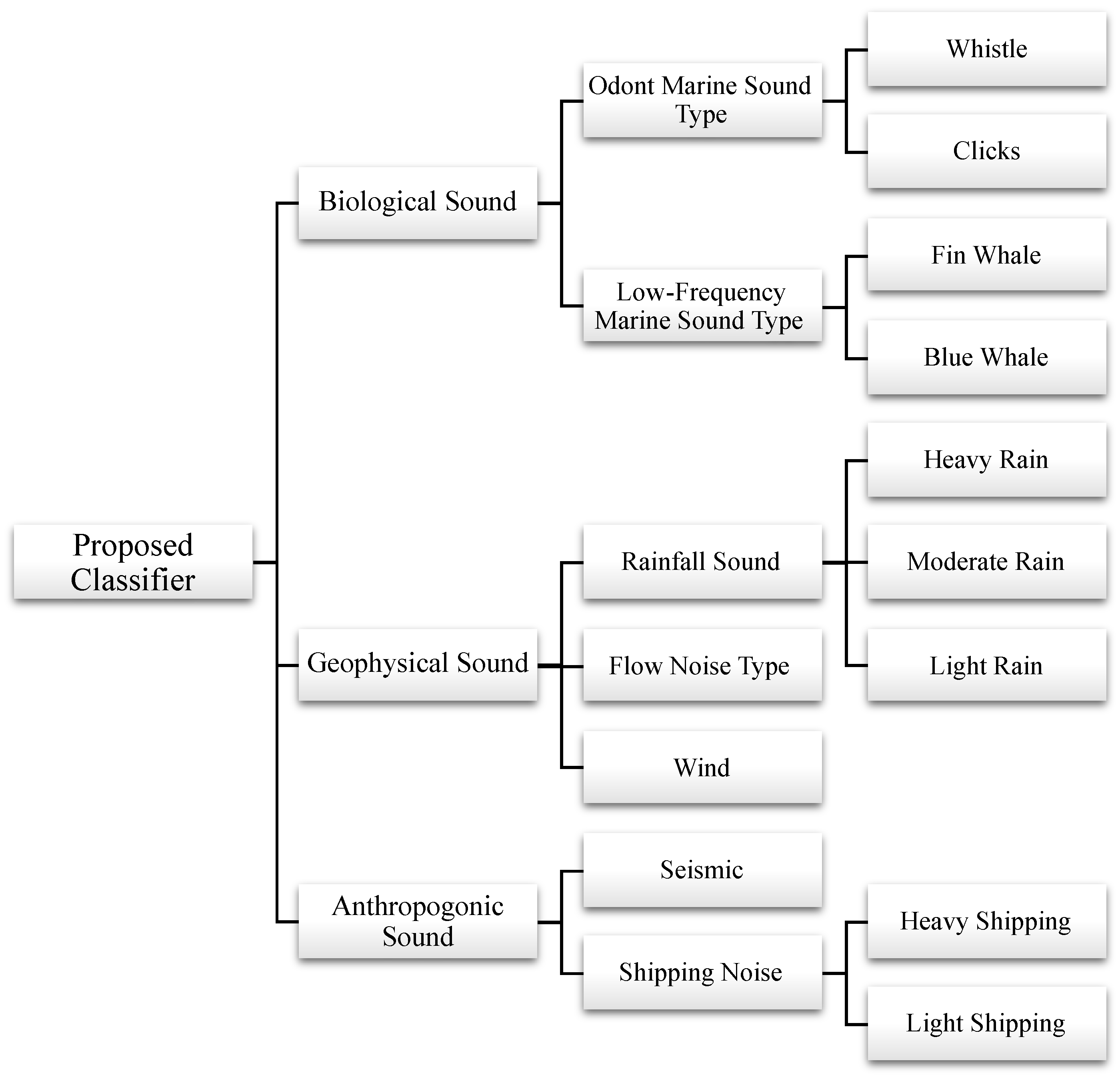
The classification algorithm automatically categorizes the soundscape into three distinct classifications, namely geophysical, biological, and anthropological, as shown in Figure 6. Geophysical sounds include those generated by natural processes such as flow noise, wind, and rainfall. Biological sounds encompass acoustic signals from marine mammals, including fin whales, blue whales, and dolphins, while anthropological sounds refer to noise created by human activities, such as shipping and seismic surveys. This comprehensive algorithm provides a detailed classification system that not only identifies the acoustic sources but also helps in monitoring the underwater environment effectively by categorizing soundscapes based on their origin.

4.4.1. Geophysicallt Generated Sound Sources

This section delves into the detection mechanism for flow noise [55], presenting models to identify its characteristics. Then, an improved wind speed estimation algorithm is described. Finally, the proficiency of the algorithm in detecting and categorizing rainfall sounds is detailed, offering insights into heavy, moderate, and light rainfall.

Flow Noise

To identify flow noise in the proposed algorithm, the boolean variable ${\mathrm{F}}_p$ (flow present) is expressed as

$$\begin{array}{cc}\hfill {\mathrm{F}}_p=& (R_{\mathrm{flow}}^2>0.95)\wedge ({\alpha }_1<m_{\mathrm{flow}}<{\alpha }_2)\hfill \\ \hfill & \vee ({\overline{\mathrm{PSD}}}_{30 \mathrm{Hz}}>{\alpha }_3)\wedge ({\overline{\mathrm{PSD}}}_{30 \mathrm{Hz}}>{\overline{\mathrm{PSD}}}_{\mathrm{HS}}+{\alpha }_4)\hfill \end{array}$$

(3)

where ∧ is the logical AND operator and ∨ is the logical OR operator. $R_{\mathrm{flow}}^2$ represents the coefficient of determination resulting from linear regression on PSDs within the frequency range of 5 to 50 Hz. $m_{\mathrm{flow}}$ is the slope of the linear regression line derived from fitting PSDs within the GA-determined frequency range. ${\overline{\mathrm{PSD}}}_{30 \mathrm{Hz}}$ signifies the mean PSD within the frequency range of 25 to 35 Hz. ${\overline{\mathrm{PSD}}}_{\mathrm{HS}}$ is the mean PSD for heavy shipping activities within the frequency range of 49 to 79 Hz. The values for thresholds (${\alpha }_1=-20$, ${\alpha }_2=-15$, ${\alpha }_3=75$, and ${\alpha }_4=10$) were optimized by the GA.

The logical operators ∧ (logical AND) and ∨ (logical OR) combine these conditions to determine the presence of flow noise. Specifically, Equation (3) asserts that if the regression fit is strong ($R_{\mathrm{Flow}}^2>0.95$) and the slope falls within a specified range, or if the mean PSD at 30 Hz exceeds a threshold and is greater than the mean PSD for heavy shipping with an additional threshold, then flow noise is considered present.

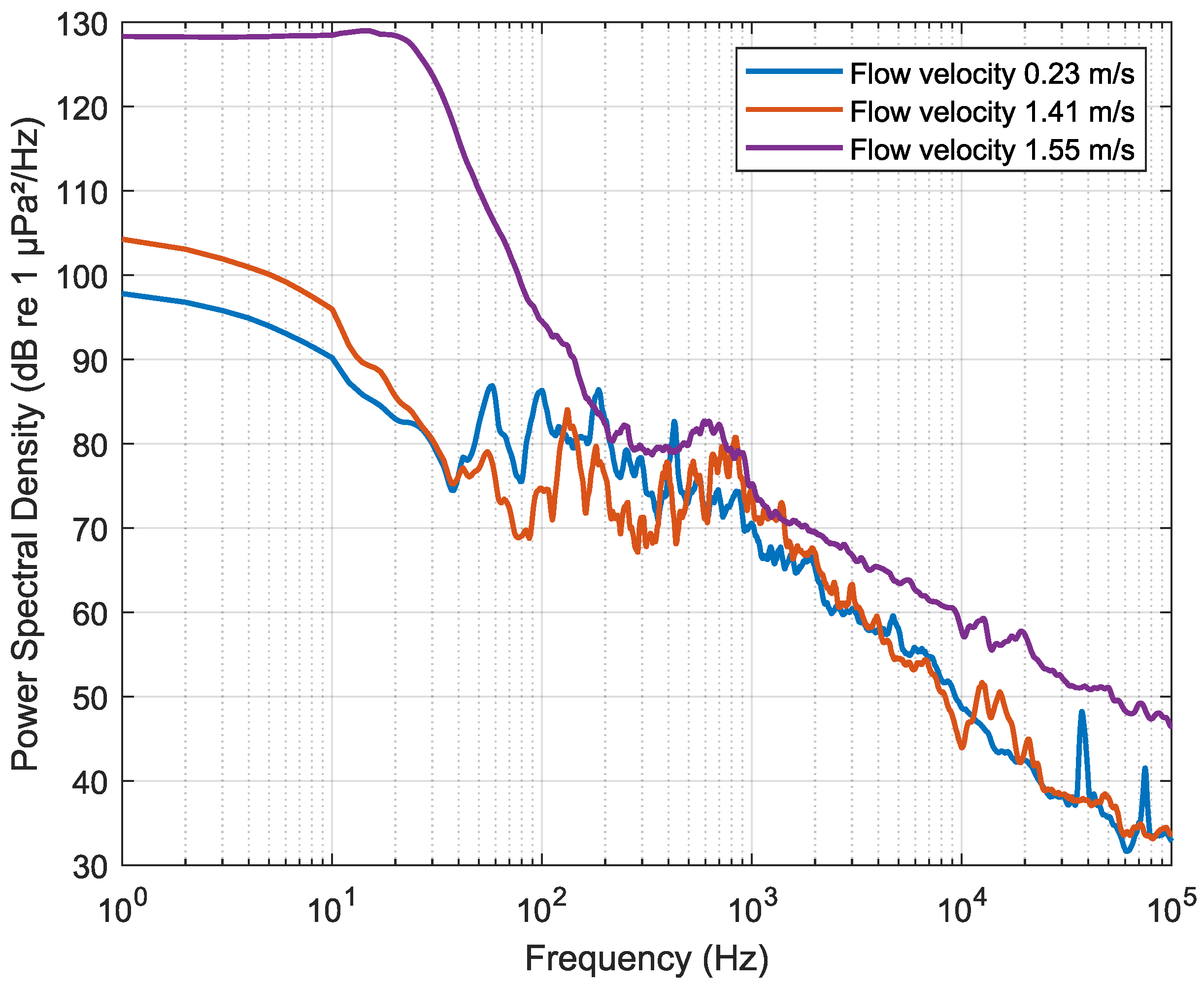
Figure 7 illustrates the correlation between flow velocity and the associated flow noise. The observed negative slope in PSD from 5 to 50 Hz and evident PSD levels exceeding $70\mathrm{dB}\mathrm{re}1\mathsf{\mu }{\mathrm{Pa}}^2/\mathrm{Hz}$ indicate an increased likelihood of flow noise with higher flow velocity.

Wind

In this work, PSD levels of wind noise, corresponding to wind speeds ranging from 0 to 14 m/s, were categorized into seven groups, with each category spanning a 2 m/s interval. An eighth category is incorporated for wind speeds exceeding 14 m/s. Figure 8 displays the average PSD estimates for each wind speed category at deep locations. The shaded area surrounding each average PSD visually represents the frequency-dependent standard deviation. To enhance clarity, the shaded regions around the average PSDs depict one-quarter of the standard deviation. The correlation between PSD levels within the 4–15 kHz frequency range and varying wind speeds, as inspired by [5], is expressed as ${\widehat{\mathrm{PSD}}}_w$ and is modeled by

$$\begin{array}{c}\hfill {\widehat{\mathrm{PSD}}}_w=m_w·{log}_{10}\left(f\right)+b_w,\end{array}$$

(4)

where PSD is the power spectral density level, f is the frequency, and $m_w$ and $b_w$ are the linear regression coefficients, which were fitted to the data.

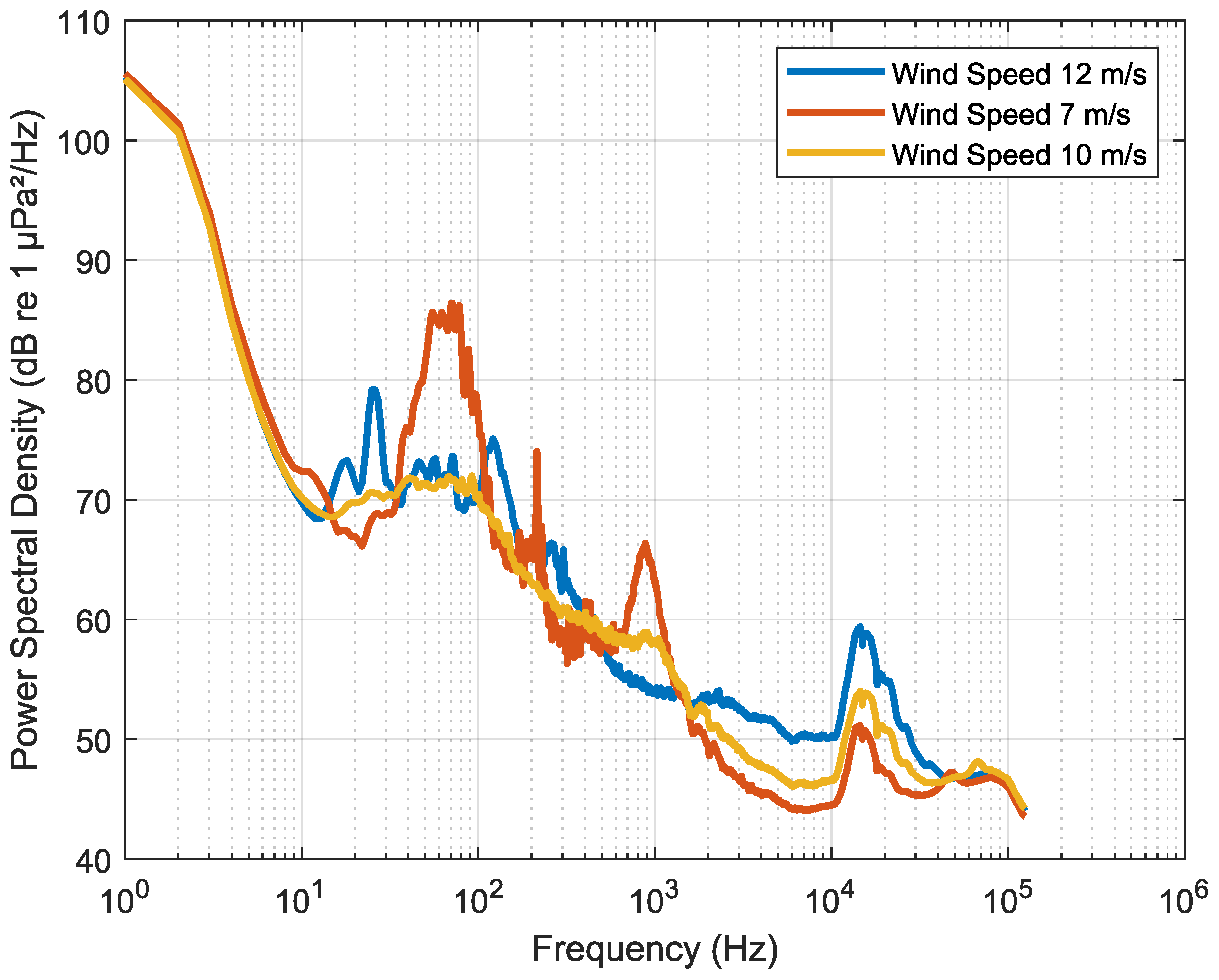
The regression curves are shown as dashed lines in Figure 8. In this figure, the PSD demonstrates a general increase in level with rising wind speeds for all frequencies. Simultaneously, the slope of the linear regression model for the 4–15 kHz frequency range experiences a decline. Applying Equation (4) to the PSD within this frequency range reveals a superior fit compared to samples of high wind speeds. To quantify the alignment of this model with Equation (4), the parameters of the regression model were measured and are detailed in

Table 2. Results of the linear regression model for the frequency range of 4–15 kHz in deep water at the Blake Plateau site.

Wind Speed (m/s)	0–2	2–4	4–6	6–8	8–10	10–12	12–14	Over 14
R-Squared	0.8904	0.9477	0.9775	0.9849	0.9867	0.9888	0.9903	0.9951
Slope (dB/decade)	−7.632	−10.08	−13.73	−15.82	−16.73	−17.72	−18.51	−23.08

.

As wind speed increases, the R-Squared values generally increase, indicating an improvement in the model fit. The highest R-squared value is 0.9951 for wind speeds over 14 m/s, suggesting a strong fit in that range. The negative slope values suggest a decreasing trend in PSD as wind speed increases. The steepest decline is observed for wind speeds over 14 m/s, with a slope of −23.08 dB/decade.

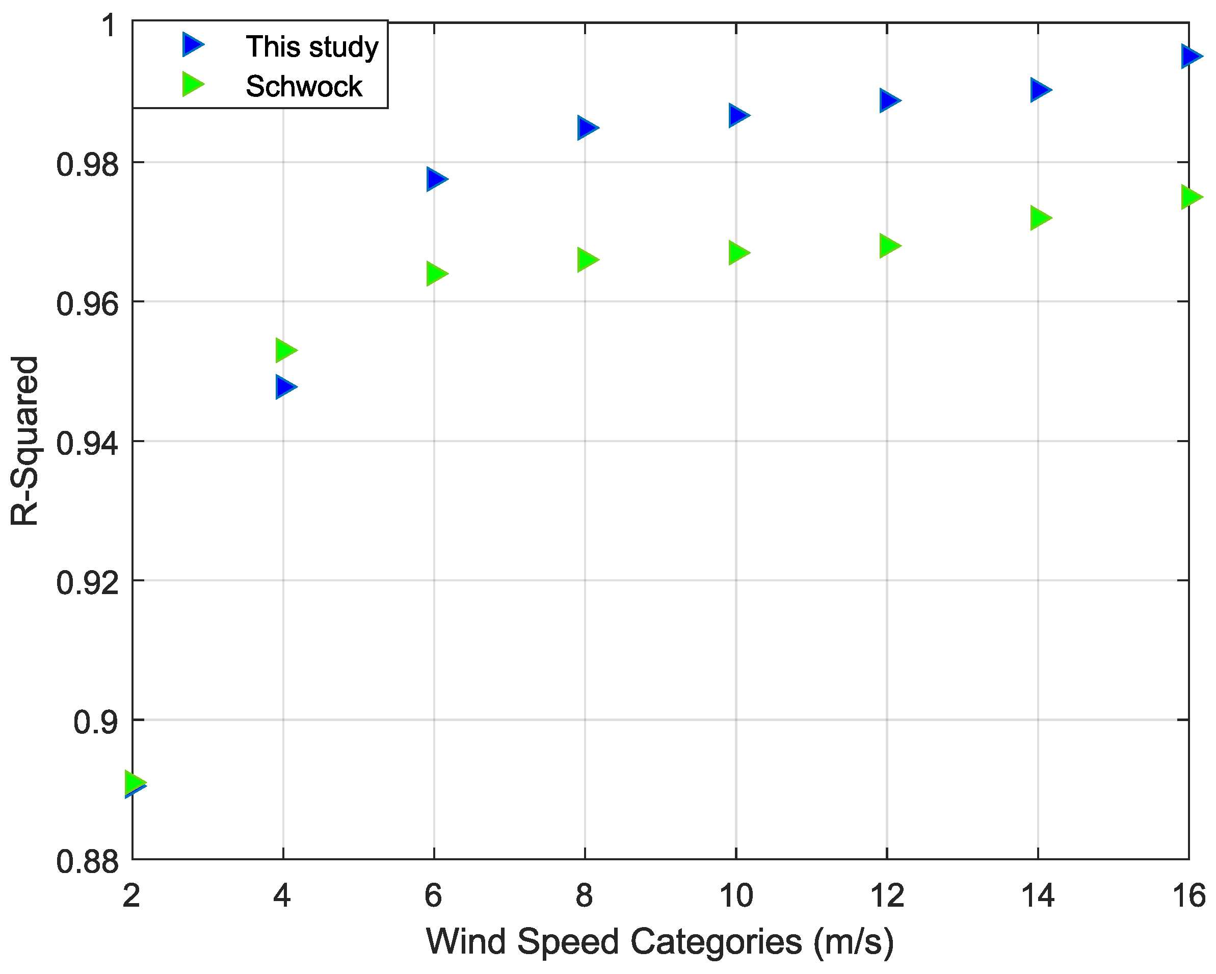
To ensure the reliability of the chosen frequency range for categorizing wind speed, a comparison is made between the R-squared values of our regression model and Schwock’s work [5], which was conducted in deep water within the frequency range of 3–25 kHz, as depicted in Figure 9. It can be observed that the proposed algorithm provides better accuracy in fitting the regression model of the PSD for wind speeds exceeding 4 m/s when compared to our chosen frequency range. This emphasizes the superiority of the proposed algorithm for the categorization of wind speed in the 4–15 kHz range.

Drizzle

Raindrop size naturally influences splash and sound. Studies identified different acoustics by different raindrop sizes, with small drops (<0.8 mm) producing gentle splashes, (0.8–1.2 mm) generating loud sounds due to bubbles, and large drops (>3.5 mm) creating energetic splashes with a loud, low-frequency sound. [56]. These findings contribute to understanding the distinct underwater “sound of drizzle” between 13 and 25 kHz, associated with small raindrops across various rainfall types, as shown in Figure 3.

The automated classification for drizzle involves examining the following conditions to identify the peak PSD at 15 kHz (${\mathrm{PSD}}_{15\mathrm{kHz}}$).

$$\mathrm{If} R^2<0.95 \mathrm{and} \left\{\begin{array}{c}{\mathrm{PSD}}_{15\mathrm{kHz}} - {\mathrm{PSD}}_{10\mathrm{kHz}} > \alpha ,\hfill \\ {\mathrm{PSD}}_{15\mathrm{kHz}} > {\mathrm{PSD}}_{20\mathrm{kHz}},\hfill \end{array}\right.\mathrm{then} \mathrm{drizzle} \mathrm{is} \mathrm{present}.$$

(5)

Here, ${\alpha }_d$ was determined to be $7\mathrm{dB}\mathrm{re}1\mathsf{\mu }{\mathrm{Pa}}^2/\mathrm{Hz}$ using the GA to minimize the loss function between the manual and automated algorithms.

Figure 10 illustrates the PSD as a function of frequency for three recorded cases in Cook Strait, as collected in 2016, each associated with different wind speeds. It can be noted that peaks at a frequency of 15 kHz are observed in all three cases, indicating the occurrence of drizzle during these specific timeframes. The classification has been validated through both manual and automated analyses. Furthermore, a discernible relationship between wind speed and drizzle is apparent. With increasing wind speed, the 15 kHz PSD peak is observed to have higher PSD values. This phenomenon is attributed to the intensified turbulence generated by stronger winds, which leads to increased agitation and the mixing of water masses. Consequently, there is greater acoustic energy at higher frequencies, such as 15 kHz.

Heavy Rain

To assess the presence of heavy rain, the boolean variable $\mathrm{HR}$ (heavy rain) is asserted as expressed by

$$\begin{array}{cc}\hfill \mathrm{HR}=& (m<{\alpha }_1)\wedge (R_{rain}^2>{\alpha }_2)\wedge ({\beta }_{8-15\mathrm{kHz}} < {\alpha }_3)\hfill \\ \hfill & \wedge (m_{rain}<{\alpha }_4)\wedge (m<{\alpha }_5\times m_{rain})\hfill \end{array}$$

(6)

m represents the linear regression slope on the PSD levels in the frequency range of 4 kHz to 15 kHz, while $R_{\mathrm{rain}}^2$ is the R-squared value for the linear regression on the PSD level in the frequency range of high rain (2 kHz to 6 kHz), and ${\mathrm{m}}_{rain}$ is the slope of the linear regression in the same high rain frequency range as shown in Figure 3. Additionally, ${\beta }_{8-15\mathrm{kHz}}$ represents the spectral kurtosis in the frequency range of 8 kHz to 15 kHz. The conditions for heavy rain involve comparisons between these parameters and optimized constants (${\alpha }_1,{\alpha }_2,{\alpha }_3,{\alpha }_4,{\alpha }_5$) using logical operations, with the constants having been determined through optimization by the GA and assigned the unitless values of −19, 0.955, 2.57, −5.2, and 1.5, respectively.

Moderate Rain

To identify moderate rain, similar analyses are conducted as those for heavy rain, involving the frequency range of 4 kHz to 15 kHz and 2 kHz to 6 kHz, as well as specific frequencies of 6 kHz, 8 kHz, and 10 kHz. Specifically, the boolean variable MR indicates that moderate rain is detected and is expressed as

$$\begin{array}{cc}\hfill \mathrm{MR}=& (R_{Rain}^2>{\alpha }_1)\wedge (m_{rain}>{\alpha }_2)\wedge (m_{rain}<{\alpha }_3)\hfill \\ \hfill & \wedge ({\beta }_{8-15\mathrm{kHz}} < {\alpha }_4)\wedge (\min ({\mathrm{PSD}}_{6\mathrm{kHz}},{\mathrm{PSD}}_{8\mathrm{kHz}},{\mathrm{PSD}}_{10\mathrm{kHz}})>{\alpha }_5)\hfill \\ \hfill & \wedge (\max ({\mathrm{PSD}}_{6\mathrm{kHz}},{\mathrm{PSD}}_{8\mathrm{kHz}},{\mathrm{PSD}}_{10\mathrm{kHz}})<{\alpha }_6),\hfill \end{array}$$

(7)

where the parameters of the slope, $R_{\mathrm{Rain}}^2$, ${\mathrm{m}}_{\mathrm{rain}}$, ${\beta }_{8-15\mathrm{kHz}}$ are defined the same as for Equation (6). The conditions for moderate rain involve specific comparisons between these parameters and the optimized constants (${\alpha }_1,{\alpha }_2,{\alpha }_3,{\alpha }_4,{\alpha }_5,{\alpha }_6$), which are assigned the values of 0.95, −10, 0, 2.5, 52, and 70, respectively. Furthermore, ${\mathrm{PSD}}_{6\mathrm{kHz}}$, ${\mathrm{PSD}}_{8\mathrm{kHz}}$, and ${\mathrm{PSD}}_{10\mathrm{kHz}}$ represent the PSD levels at frequencies of 6 kHz, 8 kHz, and 10 kHz, respectively. The moderate rain condition is satisfied when all specified conditions are simultaneously met.

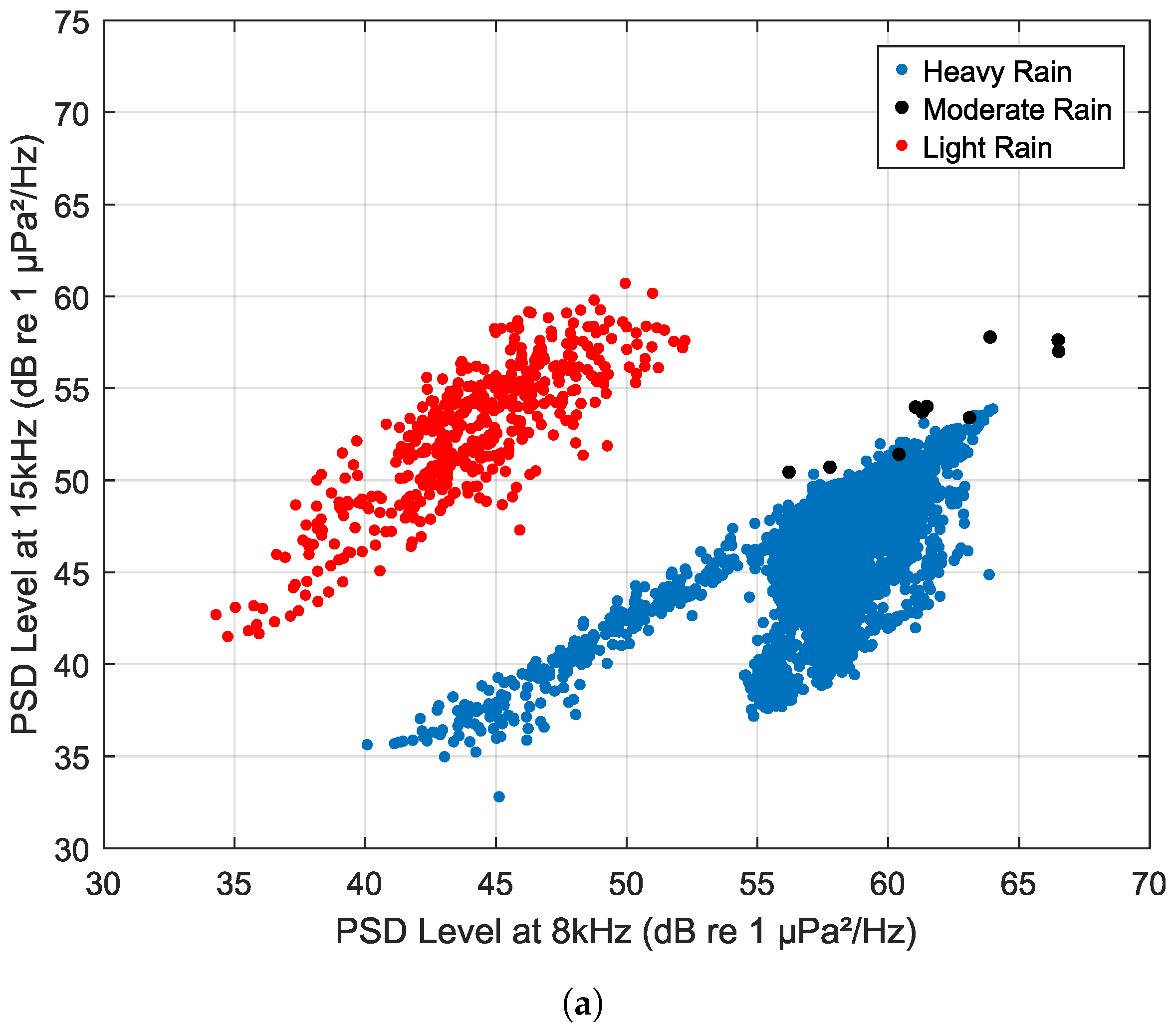
The rain classification from the Scotian Shelf dataset is presented in Figure 11. Samples for moderate rain consistently showed insufficient representation across all datasets. Despite this commonality, distinct patterns emerge among different rain classes. Subfigure (a) depicts the rain classification patterns based on the relationships between the PSD levels at 8 kHz and 15 kHz.

The analysis suggests that a two-linear regression model approach is effective in rain classification, demonstrating minimal outliers. Notably, the PSD level at 8 kHz is observed to be higher for heavy rain compared to light rain (drizzle). This distinction arises from the predominant occurrence of PSD levels at the frequency of 15 kHz during light rain conditions.

In Figure 11b, rain classification is achieved based on the slope of the regression line fitted to the PSD level for the frequency range of 8–15 kHz and the PSD level at 15 kHz. Interestingly, this classification also follows a two-horizontal regression model, indicating a powerful method for categorizing rain based on the mentioned features.

The validity of Figure 11 is established through verification by both manual and automated classification algorithms. Consequently, it is inferred that the slope of the regression of PSD levels for the frequency range of 8–15 kHz exhibits distinct characteristics for different rain intensities. Specifically, a slope higher than −10 dB/dec indicates drizzle, while a slope between −10 dB/dec and −20 dB/dec corresponds to moderate rain, and a slope lower than −20 dB/dec characterizes heavy rain. This analysis contributes valuable insights into the nuanced relationship between rain characteristics and underwater acoustics, paving the way for enhanced rain classification methodologies in underwater environments.

4.4.2. Biologically Generated Sound Sources

In this study, the underwater biological soundscape is categorized into three distinct sources: clicks and whistles produced by dolphins and the moan-type sounds emitted by fin whales and blue whales. In this section, we will examine these various types of underwater biological sound sources.

Click

Although click peak frequencies vary among dolphin species, many dolphin species produce clicks with peak energy in the 25–40 kHz range [57,58]. As such, this work confirms the detection of dolphin clicks (DCs) if the boolean variable DC is asserted. It is defined as

$$\begin{array}{c}\hfill \mathrm{DC}=\left({\mathrm{PSD}}_{30 \mathrm{kHz}}>{\mathrm{PSD}}_{20 \mathrm{kHz}}\right)\wedge \left({\mathrm{PSD}}_{30 \mathrm{kHz}}>{\alpha }_1\right)\wedge \left({\beta }_{20-30 \mathrm{kHz}}>{\alpha }_2\right).\end{array}$$

(8)

Suppose the PSD at 30 kHz (${\mathrm{PSD}}_{30 \mathrm{kHz}}$) surpasses that at 20 kHz (${\mathrm{PSD}}_{20 \mathrm{kHz}}$), and ${\mathrm{PSD}}_{30 \mathrm{kHz}}$ is also higher than a specified threshold (${\alpha }_1$), while also having the spectral kurtosis in the frequency range of 20 to 30 kHz (${\beta }_{20-30 \mathrm{kHz}}$) exceed the threshold (${\alpha }_2$); then it is inferred that Dolphin clicks have been observed. In this work, ${\alpha }_1$ and ${\alpha }_2$ are optimized to be 48 dB and 2.06, respectively.

Whistle

The analysis of the whistle soundscape is performed within the frequency range of 8 to 15 kHz [59,60]. This is achieved by assessing if the boolean variable $\mathrm{DW}$ meets the following conditions:

$$\begin{array}{c}\hfill \mathrm{DW}=(R_{\mathrm{W}}^2<{\alpha }_1)\wedge ({\max }_{\mathrm{PSD}}>{\alpha }_2)\wedge ({\beta }_{8-15 \mathrm{kHz}} > {\alpha }_3)\wedge (m_w>{\alpha }_4)\end{array}$$

(9)

In the context of this analysis, $R_{\mathrm{W}}^2$ represents the R-squared value derived from the regression model for PSD levels within the frequency range of 5–15 kHz. The term $m_w$ refers to the slope of the regression model applied to the PSD level on this frequency range. Additionally, ${\beta }_{8-15 \mathrm{kHz}}$ signifies the spectral kurtosis of PSD within the frequency range of 8–15 kHz. The variable ${\max }_{\mathrm{PSD}}$ is defined as the maximum value among ${\mathrm{PSD}}_{10 \mathrm{kHz}},{\mathrm{PSD}}_{12 \mathrm{kHz}}$, and ${\mathrm{PSD}}_{15 \mathrm{kHz}}$. These parameters collectively contribute to whistle detection. The optimized values for ${\alpha }_1$, ${\alpha }_2$, ${\alpha }_3$, and ${\alpha }_4$ are 0.95, 46 dB, 2, and −12 dB/dec, respectively.

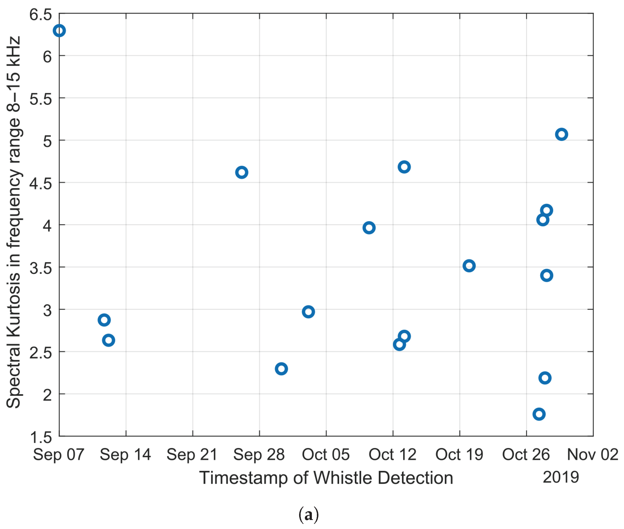
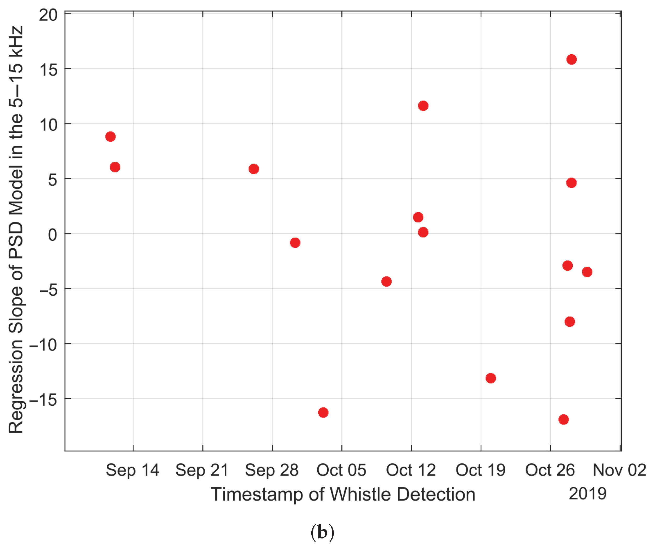
A comparative analysis was conducted to assess the effectiveness of both manual analysis and an automatic algorithm for whistle detection, as depicted in Figure 12, based on the manual analysis of the Gaspe (Site B) dataset. The x-axis represents the date and time when the user observed the whistle through PAMlab analysis. Static calculations of the millidecade recorded data determine the y-axis. Figure 12a illustrates the spectral kurtosis variations within the frequency range of 8–15 kHz during the observation of the whistle. This figure validates the condition of the whistle detection algorithm, where ${\beta }_{8-15 \mathrm{kHz}}>2$. Additionally, Figure 12b displays the linear regression slope of PSD within the 5–15 kHz frequency range observed during the whistle. This figure demonstrates that the slope must be greater than −12 dB/Dec for the whistle detection algorithm, as shown in Equation (9). This helps distinguish whistle data from other sources.

Fin and Blue Whale

Fin whales worldwide produce songs whose dominant notes have a peak frequency in the 20–22 Hz range [61]. Blue whales show more variability in song features worldwide, with note peak frequencies ranging from 17 Hz to 65 Hz [62]. To identify fin and blue whales, it is necessary to exclude samples related to shipping activity that occurred at the same timestamp. Subsequently, the following set of equations is examined. The blue whale (BW) is observed if the condition in Equation (10) is met.

$$\begin{array}{c}\hfill \mathrm{BW}=({\mathrm{bw}}_1>{\alpha }_1)\vee ({\mathrm{bw}}_2>{\alpha }_2),\end{array}$$

(10)

The presence of the fin whale (FW) is confirmed if the condition in Equation (11) is satisfied.

$$\begin{array}{ll}\mathrm{FW}& =(\mathrm{fw}>{\alpha }_3)\wedge ({\overline{\mathrm{PSD}}}_{20 \mathrm{Hz}}>({\overline{\mathrm{PSD}}}_{18 \mathrm{Hz}}+{\alpha }_4)\\ & \wedge ({\overline{\mathrm{PSD}}}_{20 \mathrm{Hz}}>{\overline{\mathrm{PSD}}}_{25 \mathrm{Hz}})\wedge ({\overline{\mathrm{PSD}}}_{20 \mathrm{Hz}}<{\alpha }_5),\end{array}$$

(11)

The intermediate variables ${\mathrm{bw}}_1$, ${\mathrm{bw}}_2$, and fw are calculated based on

$$\begin{array}{cc}\hfill \mathrm{fw}& ={\displaystyle \frac{3\times ({\mathrm{PSD}}_{21 \mathrm{Hz}}+{\mathrm{PSD}}_{22 \mathrm{Hz}})}{({\mathrm{PSD}}_{11 \mathrm{Hz}}+{\mathrm{PSD}}_{12 \mathrm{Hz}}+{\mathrm{PSD}}_{13 \mathrm{Hz}}+{\mathrm{PSD}}_{33 \mathrm{Hz}}+{\mathrm{PSD}}_{34 \mathrm{Hz}}+{\mathrm{PSD}}_{35 \mathrm{Hz}})}},\hfill \\ \hfill {\mathrm{bw}}_1& ={\displaystyle \frac{3\times ({\mathrm{PSD}}_{16 \mathrm{Hz}}+{\mathrm{PSD}}_{17 \mathrm{Hz}})}{({\mathrm{PSD}}_{11 \mathrm{Hz}}+{\mathrm{PSD}}_{12 \mathrm{Hz}}+{\mathrm{PSD}}_{13 \mathrm{Hz}}+{\mathrm{PSD}}_{23 \mathrm{Hz}}+{\mathrm{PSD}}_{24 \mathrm{Hz}}+{\mathrm{PSD}}_{25 \mathrm{Hz}})}},\hfill \\ \hfill {\mathrm{bw}}_2& ={\displaystyle \frac{3\times ({\mathrm{PSD}}_{43 \mathrm{Hz}}+{\mathrm{PSD}}_{44 \mathrm{Hz}})}{({\mathrm{PSD}}_{36 \mathrm{Hz}}+{\mathrm{PSD}}_{37 \mathrm{Hz}}+{\mathrm{PSD}}_{38 \mathrm{Hz}}+{\mathrm{PSD}}_{49 \mathrm{Hz}}+{\mathrm{PSD}}_{50 \mathrm{Hz}}+{\mathrm{PSD}}_{51 \mathrm{Hz}})}},\hfill \end{array}$$

(12)

where the symbol ${\overline{\mathrm{PSD}}}_{i \mathrm{Hz}}$ represents the PSD at frequencies around i. The logical OR operation is denoted by ∨. The parameters ${\alpha }_1$, ${\alpha }_2$, ${\alpha }_3$, ${\alpha }_4$, and ${\alpha }_5$ are optimized thresholds with the following values: 2, 1.2, 1.04, 4, and 105 dB, respectively.

4.4.3. Anthropogenically Generated Sound Sources

This study classifies shipping activities into two types: heavy shipping and light shipping. As illustrated in Figure 3, heavy shipping exhibits a peak frequency within the range of 50 to 80 Hz, while light shipping is analyzed in the frequency range of 100 to 400 Hz. This section explains the methodologies employed to discern the type of shipping activity.

Shipping activities are categorized as “Heavy” or “Light” based on conditions involving average PSD in different frequency ranges and spectral kurtosis for the frequency range of 49 to 500 Hz. Satisfying (13) confirms the occurrence of shipping activities, whether heavy or light.

$$\begin{array}{c}\hfill ({\overline{\mathrm{PSD}}}_{30 \mathrm{Hz}}<{\alpha }_1)\wedge ({\beta }_{50-500} > {\alpha }_2)\wedge ({\beta }_{50-500} < {\alpha }_3),\end{array}$$

(13)

where the average PSD level for the frequency range of 25 to 33 Hz is denoted as ${\overline{\mathrm{PSD}}}_{30 \mathrm{Hz}}$. The spectral kurtosis in the frequency range of 50 to 500 Hz is denoted as ${\beta }_{50-500}$. Firstly, the mentioned conditions must be assessed for both “Heavy” and “Light”. If these conditions are satisfied, the identification of either heavy shipping or light shipping is further examined using the corresponding conditions. To determine the presence of heavy shipping, the boolean variable HS is defined as

$$\begin{array}{c}\hfill \mathrm{HS}=(d_1>{\alpha }_4)\wedge (d_1<{\alpha }_5)\wedge (d_2>{\alpha }_6)\wedge (d_2<{\alpha }_7)\\ \hfill \wedge ({\overline{\mathrm{PSD}}}_{\mathrm{HS}}>{\alpha }_8)\wedge ({\overline{\mathrm{PSD}}}_{\mathrm{HS}}>{\overline{\mathrm{PSD}}}_{\mathrm{LS}}).\end{array}$$

(14)

Also, by taking into account the boolean variable LS for light shipping, the detection of light shipping activity occurs when LS is asserted. LS is defined as

$$\begin{array}{c}\hfill \mathrm{LS}=(d_1^{\prime }>{\alpha }_4)\wedge (d_1^{\prime }<{\alpha }_5)\wedge (d_2^{\prime }<{\alpha }_6)\wedge (d_2^{\prime }>{\alpha }_7)\\ \hfill \wedge ({\overline{\mathrm{PSD}}}_{\mathrm{LS}}>{\alpha }_9)\wedge ({\overline{\mathrm{PSD}}}_{\mathrm{LS}}>{\overline{\mathrm{PSD}}}_{\mathrm{HS}}),\end{array}$$

(15)

where parameters ${\alpha }_1$ to ${\alpha }_9$ were optimized to the best value by the GA as detailed in

Table 3. Optimized parameter values by the GA.

Parameters	${\mathit{\alpha }}_1$	${\mathit{\alpha }}_2$	${\mathit{\alpha }}_3$	${\mathit{\alpha }}_4$	${\mathit{\alpha }}_5$	${\mathit{\alpha }}_6$	${\mathit{\alpha }}_7$	${\mathit{\alpha }}_8$	${\mathit{\alpha }}_9$
Values	103	2.8	14.5	−4.5	12.6	−1.9	14.5	73	69

. The calculations for $d_1$, $d_2$, $d_1^{\prime }$, and $d_2^{\prime }$ are outlined as

$$\begin{array}{cc}\hfill d_1& ={\overline{\mathrm{PSD}}}_{\mathrm{HS}}-{\overline{\mathrm{PSD}}}_{30 \mathrm{Hz}},\hfill \end{array}$$

(16)

$$\begin{array}{cc}\hfill d_2& ={\overline{\mathrm{PSD}}}_{\mathrm{HS}}-{\overline{\mathrm{PSD}}}_{100 \mathrm{Hz}},\hfill \end{array}$$

(17)

$$\begin{array}{cc}\hfill d_1^{\prime }& ={\overline{\mathrm{PSD}}}_{\mathrm{LS}}-{\overline{\mathrm{PSD}}}_{100 \mathrm{Hz}},\hfill \end{array}$$

(18)

$$\begin{array}{cc}\hfill d_2^{\prime }& ={\overline{\mathrm{PSD}}}_{\mathrm{LS}}-{\overline{\mathrm{PSD}}}_{100–400 \mathrm{Hz}}.\hfill \end{array}$$

(19)

where ${\overline{\mathrm{PSD}}}_{\mathrm{HS}}$ is the mean PSD for heavy shipping activities within the frequency range of 49 to 79 Hz (optimized by the GA), and ${\overline{\mathrm{PSD}}}_{\mathrm{LS}}$ is the mean PSD for light shipping activities within the frequency range of 360 to 448 Hz (optimized by GA). ${\overline{\mathrm{PSD}}}_{100 \mathrm{Hz}}$ and ${\overline{\mathrm{PSD}}}_{100-400 \mathrm{Hz}}$ present the average PSD level for the frequency ranges of 89 to 103 Hz and 107 to 408 Hz, respectively (both optimized by the GA).

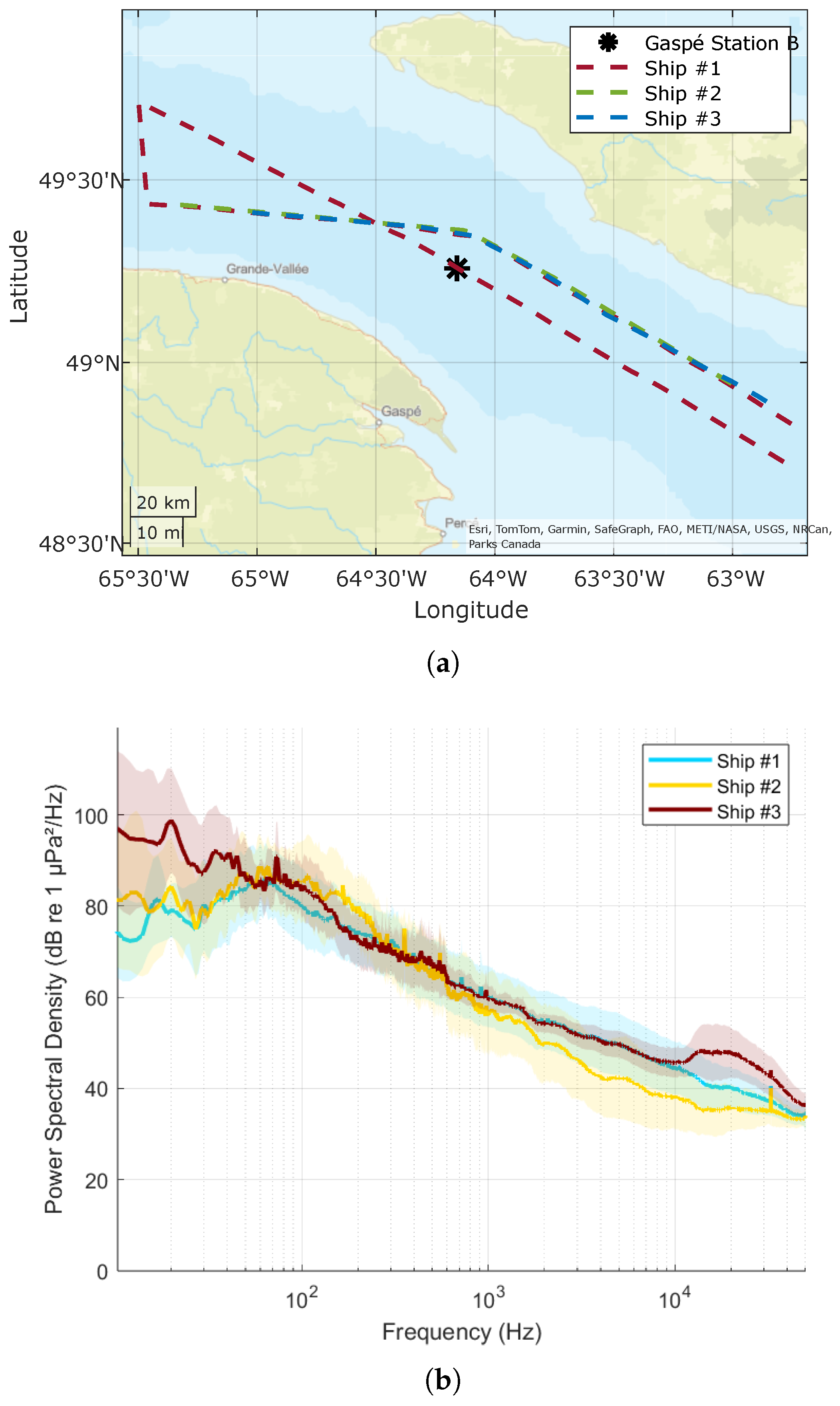
To assess the accuracy of shipping activity detection, three ships were chosen for tracking using the AIS dataset. The PSDs when the ships passed around Gaspé Station B in 2019 were recorded, as shown in Figure 13b. Relevant AIS data for these ships is compiled in

Table 4. AIS information of three ships.

Number	Duration	Class
1	14 September 2019 17:03:31 to 6 October 2019 21:39:09	Cargo
2	11 October 2019 08:48:48 to 11 October 2019 19:12:38	Passenger
3	18 October 2019 11:23:07 to 18 October 2019 18:22:41	Tanker

. The prominent peak observed in the frequency range of 49 to 79 Hz serves as a clear indicator of heavy shipping activity in the region, aligning with established patterns of maritime traffic. Interestingly, the identified peaks around 20 Hz offer compelling evidence for the presence of fin whales, which are known for emitting acoustic signals within this frequency range. This demonstrates that the algorithm can detect multiple sources within the one-minute spectrum. These distinctive spectral features not only confirm the heavy shipping dynamics but also highlight the coexistence of marine life, specifically fin whales, in the study area. This detailed frequency analysis enhances our understanding of the acoustic environment, enabling an assessment of both shipping and marine life dynamics in the vicinity of Gaspé Station B.

4.5. Classifier Performance

The performance evaluation of the proposed classification algorithm requires the computation of precision (positive predictive value), which is given by

$$\mathrm{Precision}={\displaystyle \frac{n_{TP}}{n_{TP}+n_{FP}}},$$

(20)

where $n_{TP}$ represents the number of true positives, $n_{FP}$ represents the number of false positives, and $n_{FN}$ represents the number of false negatives. Recall (sensitivity or the true predictive rate) is expressed as

$$\mathrm{Recall}={\displaystyle \frac{n_{TP}}{n_{TP}+n_{FN}}},$$

(21)

while the ${\mathrm{F}}_{\gamma }$ score (the harmonic mean of precision and recall) is expressed as

$$F_{\gamma }={\displaystyle \frac{(1+{\gamma }^2)·\mathrm{Precision}·\mathrm{Recall}}{({\gamma }^2·\mathrm{Precision})+\mathrm{Recall}}}$$

(22)

Note that $\gamma$ is a parameter that controls the relative importance of precision and recall in the evaluation of a model’s performance. When $\gamma =1$, it is equivalent to the F1 score, giving equal weight to precision and recall. When $\gamma <1$, it emphasizes precision more; when $\gamma >1$, it emphasizes recall more. The Matthews Correlation Coefficient (MCC) is specifically designed to account for the four essential components of a confusion matrix and is calculated using

$$\begin{array}{cc}\hfill \mathrm{MCC}& ={\displaystyle \frac{n_{TP}·n_{TN}-n_{FP}·n_{FN}}{\sqrt{(n_{TP}+n_{FP})(n_{TP}+n_{FN})}}}·\hfill \\ \hfill & {\displaystyle \frac{1}{\sqrt{(n_{TN}+n_{FP})(n_{TN}+n_{FN})}}},\hfill \end{array}$$

(23)

where $n_{TN}$ represents the number of true negatives.

Table 5. Classification results in % for the proposed algorithm.

Source Type	Precision	Recall	${\mathbf{F}}_1$	MCC	${\mathbf{F}}_{0.5}$	Occurrence
Flow noise	91.30	79.24	84.84	71.37	88.60	510
Heavy rain	72.09	100	83.78	77.40	76.35	112
Light rain	81.81	100	90	89.47	84.90	150
Fin whale	100	77.78	78.9	77.5	94.59	30
Whistle	92.38	70.58	80	77.57	86.95	173
Clicks	93.75	99.8	96.77	96.26	94.93	112
Shipping activity	90.03	78.73	83.04	69.83	87.55	1048

provides a wide overview of the performance percentages achieved by our classification algorithm across various sound source types. The evaluation metrics include precision, recall, the ${\mathrm{F}}_1$ score, the Matthews Correlation Coefficient (MCC), and the ${\mathrm{F}}_{0.5}$ Score. Additionally, the column “Occurrence” displays the frequency of each source in the manual data collection.

The algorithm demonstrates good precision in identifying several sound sources. Notably, it excels in precision for “Fin whale” (100%), “Clicks” (93.75%), “Whistle” (92.38%), and “Flow noise” (91.30%). This indicates a high degree of accuracy in classifying instances as positive for these specific sound sources.

“Heavy rain” and “Light rain” achieve perfect recall (100%), implying that the algorithm successfully identifies all positive instances of classifying rain sounds.

“Clicks” exhibit a balanced performance with an ${\mathrm{F}}_1$ score of 96.77%, showcasing a harmonious trade-off between precision and recall. This suggests that the algorithm maintains a good balance between minimizing false positives and false negatives for “Clicks.”

The Matthews Correlation Coefficient (MCC) values further emphasize the algorithm’s effectiveness. “Clicks” and “Light rain” stand out with MCC values of 96.26% and 89.47%, respectively. These values indicate a strong correlation between the algorithm’s predictions and the actual classifications, reinforcing its reliability.

The ${\mathrm{F}}_{0.5}$ score, which places more emphasis on precision, highlights the algorithm’s proficiency across different sound sources. “Fin whale” and “Clicks” particularly excel in this metric, with scores of 94.59% and 94.93%, respectively.

In summary, Table 5 reflects a good overall performance of the proposed classification algorithm in sound source identification. The high precision, recall, and balanced ${\mathrm{F}}_1$ scores across various sound sources indicate the algorithm’s versatility and effectiveness in diverse audio environments. These results underscore its potential for practical applications in sound classification scenarios. We acknowledge that performance metrics for certain classes are not reported in the table because of the low sample sizes for those classes in those datasets.

5. Quantifying the Wind Speed

While satellite-based measurements are expected to play a significant role in monitoring essential climate variables, certain factors necessitate in situ observations, such as their availability to aid in the interpretation and calibration of satellite data. The measurement of surface wind speed encounters challenges posed by destructive surface wave fields on buoys. An alternative method involves leveraging wind-generated ambient sound at ocean depth for more powerful observations. This concept was introduced by Vagle et al. [63]. Their quantitative algorithm utilizes the sound level at 8 kHz, and wind speed estimation, denoted as $v_{w,vagel}$ in m/s, is expressed as

$$\begin{array}{cc}\hfill v_{w,vagle}& ={\displaystyle \frac{{10}^{\frac{{\mathrm{SPL}}_8}{20}}+104.3}{53.91}},\hfill \end{array}$$

(24)

where ${\mathrm{SPL}}_8$ denotes the sound level at 8 kHz. This relationship is valid within the range of $3.3<v_{w,vagle}<15$ m/s. Above 15 m/s, the influence of bubble clouds absorbing sound causes an underestimation of wind speed in the 8 kHz signal. Conversely, in wind conditions below 2 m/s, where wave breaking is absent, no acoustic signal is available for measuring wind speed. The most recently proposed quantitative wind speed relationship by Nystuen is calculated as a third-order polynomial in terms of ${\mathrm{SPL}}_8$, and the speed estimate $v_{w,nystuen}$ in m/s is expressed as

$$\begin{array}{cc}\hfill v_{w,nystuen}& =a_0·{\left({\mathrm{SPL}}_8\right)}^3+a_1·{\left({\mathrm{SPL}}_8\right)}^2+a_2·{\mathrm{SPL}}_8+a_3,\hfill \end{array}$$

(25)

where the coefficients were defined to be $a_0=0.0005$, $a_1=-0.0310$, $a_2=0.4904$, and $a_3=2.0871$ [4].

In this work, a relationship between wind speed and a third-order polynomial in terms of the PSD at 6 kHz is proposed, and the value also depends on the depth of the recorder. Specifically, the estimated wind speed $v_{w,proposed}$ is expressed as

$$\begin{array}{cc}\hfill v_{w,proposed}& =b_0·{\left({\mathrm{PSD}}_6\right)}^3+b_1·{\left({\mathrm{PSD}}_6\right)}^2+b_2·{\mathrm{PSD}}_6+b_3·h,\hfill \end{array}$$

(26)

where h represents the depth of the recorder. The coefficients $b_0$, $b_1$, $b_2$, and $b_3$ are estimated to be $-2.309178\times {10}^{-5}$, $5.852897\times {10}^{-3}$, $-1.102547\times {10}^{-1}$, and $1.661\times {10}^{-4}$, respectively.

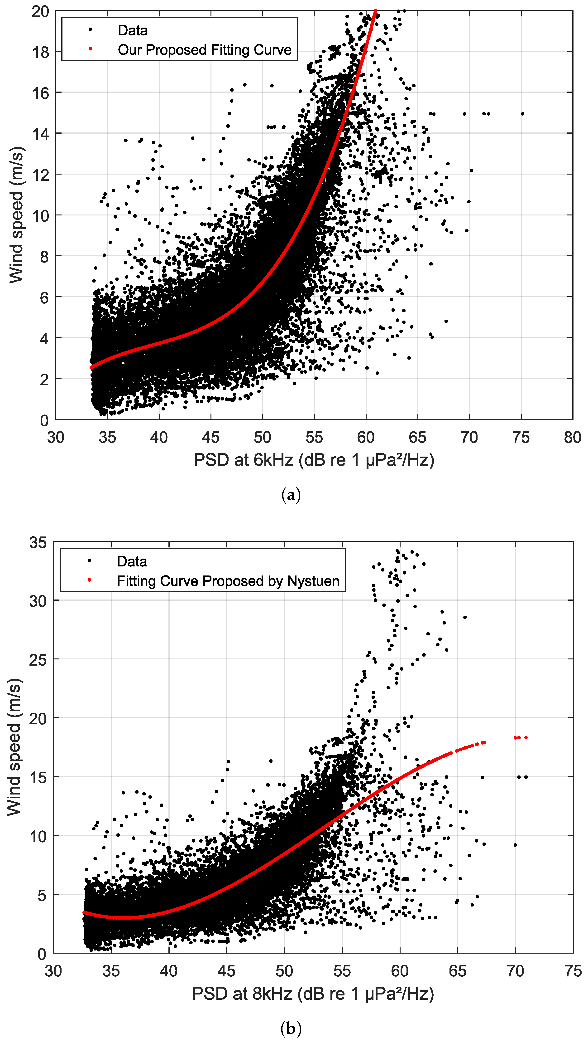
Figure 14 compares the PSD trends at 6 kHz using Equation (26) and at 8 kHz using Equation (25) with the corresponding actual wind speed. The red curves delineate the estimated wind speed derived from both the proposed algorithm (Equation (26)) and Nystuen’s algorithm (Equation (25)). As observed from Figure 14, the PSD at 6 kHz performs better in tracking wind speed trends than that at 8 kHz, which displays outliers, causing the estimated wind speed to deviate from the actual data. This observation validates that the proposed algorithm can outperform Nystuen’s algorithm in deep water conditions.

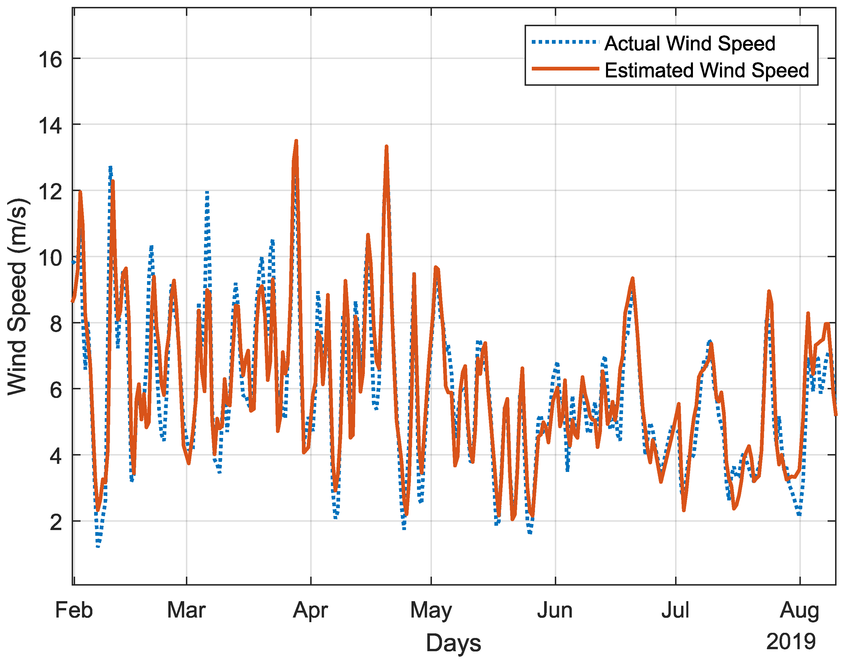
The proposed algorithm, incorporating a depth-dependent coefficient, introduces a level of flexibility for fitting, enhancing its performance. Additionally, the PSDs at 6 kHz capture more features of the wind speed, enhancing the algorithm’s performance, as illustrated in Figure 15. This figure shows a comparison between the 24 h averaged wind speed as estimated by the proposed algorithm and the actual 24 h averaged wind speed obtained from the ERA5 data spanning from February to August 2019 in the Blake Plateau. The comparison of root mean square (RMS) error among three wind speed estimation algorithms for deep water sites reveals distinct levels of accuracy. The proposed algorithm stands out with an RMS error of 1.1 m/s, indicating the smallest average discrepancy between predicted and observed wind speeds. In contrast, Vagle’s algorithm exhibits a higher error of 1.5 m/s, suggesting less precise estimations. Nystuen’s algorithm falls in between with an RMS error of 1.22 m/s, offering a moderate level of accuracy.

Model for the Ambient Sound Level Underwater from Wind (MASLUW)

To estimate wind speed from the PSD, it is necessary to remove PSD data influenced by specific soundscapes. PSDs predicted to contain heavy shipping, light shipping, light rain, heavy rain, moderate rain, whistles, sperm clicks, and whale clicks are excluded, as these soundscapes, particularly in the 6 to 8 kHz range, can interfere with accurate wind speed estimation. Consequently, an alternative method is employed, which does not rely on soundscape prediction. This approach estimates wind speed based on parameters such as water depth, sensor depth, sound speed profile, and sediment type, represented by grain size.

MASLUW [64] is a model for estimating ambient sound levels and spatial coherence using Harrison’s frequency domain formulas [65]. It generates time-series data through Fourier synthesis, incorporating surface and seabed reflection loss, ray-based propagation, and random time-series generation. The model maintains spatial coherence crucial for sonar array processing. MASLUW’s surface noise-level model uses Ainslie’s formulas [66] based on wind speed. It includes seabed reflection loss from Jensen et al. [67], ray-based propagation for accurate sound-level predictions, and seawater absorption models. The spatial coherence is computed using singular value decomposition (SVD), ensuring realistic time-series data for sonar performance modeling. The spectral density of the areic dipole source factor, $K^{\mathrm{Wind}}$, is calculated based on the frequency in kilohertz (F) [66]:

$$\begin{array}{cc}\hfill K^{\mathrm{Wind}}& ={\displaystyle \frac{{10}^{4.12}\times {\hat{v}}_{\mathrm{APL}}^{2.24}}{(1.5+F^{1.59})\times {10}^{0.1\times \delta }}}\mathsf{\mu }{\mathrm{Pa}}^2 {\mathrm{Hz}}^{-1}\hfill \end{array}$$

(27)

$$\begin{array}{cc}\hfill \delta & =\left\{\begin{array}{cc}0\hfill & \mathrm{if} \Delta T<1\hfill \\ 0.26\times {(\Delta T-1)}^2\hfill & \mathrm{if} \Delta T\ge 1\hfill \end{array}\right.\hfill \end{array}$$

where $\Delta T$ is the temperature difference in degrees Celsius:

$$\begin{array}{cc}\hfill \Delta T& ={\hat{T}}_{\mathrm{air}}-{\hat{T}}_{\mathrm{water}}\hfill \end{array}$$

(28)

${\hat{v}}_{\mathrm{APL}}$ is related to wind speed $v_{10}$ (wind speed at 10 m above the water surface in m/s) according to

$$\begin{array}{c}\hfill {\hat{v}}_{\mathrm{APL}}=\max (v_{10},1)\end{array}$$

(29)

The model compares predicted sound levels with ERA5 data, incorporating environmental factors such as water depth, sediment type, and sound speed profile. It is designed to accurately predict wind-related noise and spatial correlations, which is essential for improving sonar system performance.

First, the slopes of the averaged spectrum against ${log}_{10}\left(\mathrm{Frequency}\right)$ between 4 and 15 kHz are calculated, along with the coefficient of determination ($R^2$) for the data and the fitted line. The analysis proceeds only for hours where the $R^2$ value exceeds 0.95, indicating a strong linear fit. Additionally, the slope must fall between −13 and −19 dB/decade, allowing for a tolerance around the expected slope of −16 dB/decade. For the minutes that meet these criteria, the mean PSD at 6 kHz, 5 kHz, and 4 kHz is extracted for comparative analysis.

To generate the reference PSD data, MASLUW was executed for wind speeds ranging from 3 to 15 m/s in increments of 0.25 m/s, with $\varphi$ values from −2 to 6 [68], also spaced at 0.25 increments.

The analysis utilized the average monthly sound speeds, sound speed profiles (SSPs), and sediment-type data extracted from the DECs 2 Beta tool for September and October 2019, as shown in Figure 16. The bathymetry subfigure indicates that the sediment in the area is predominantly sandy, with a grain size parameter of $\varphi =1.5$. These characteristics play a crucial role in understanding sound propagation in the region, as both sound speed and sediment type significantly influence acoustic interactions with the seafloor.

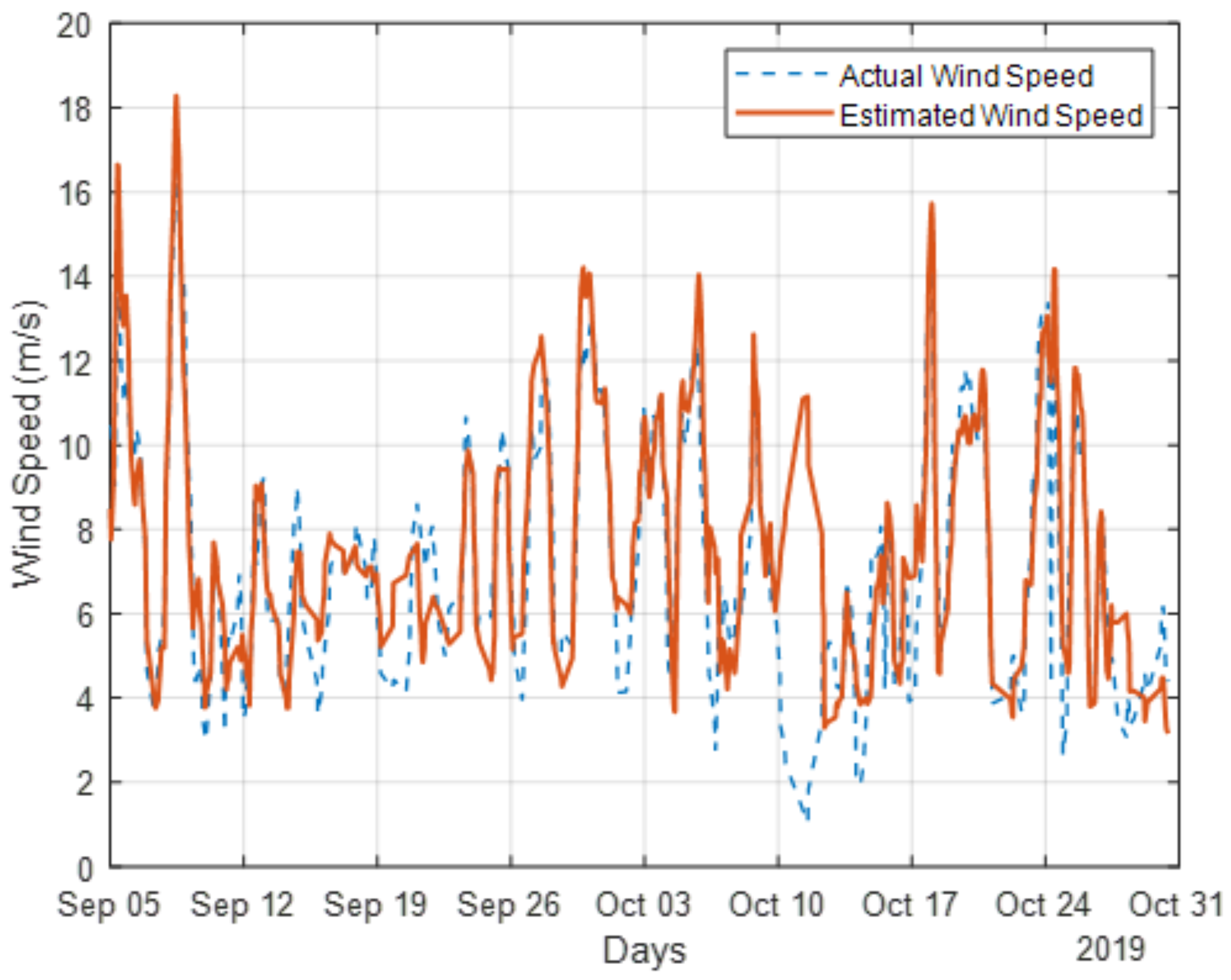
Figure 17 presents a comparison between the hourly averaged wind speed estimated by the MASLUW model and the actual hourly averaged wind speed recorded at Gaspe (Site B) during the period from September to October 2019. The estimated wind speed values from the MASLUW model demonstrate a high level of agreement with the actual measurements, with an overall error of 1.08 m/s. While the overall alignment between the MASLUW estimates and actual data is strong, slight discrepancies may be observed at higher wind speeds or during rapid fluctuations in atmospheric conditions. These deviations could be due to limitations in model resolution or external factors influencing wind patterns, which are not captured in the PSD data.

6. Conclusions

This study introduced an algorithm designed to identify common sound sources in underwater soundscapes, providing valuable insights into their presence within the marine environment. This algorithm employs easily computed metrics, specifically one-minute spectral kurtosis and power spectral density levels, offering a practical and efficient means of identifying and quantifying specific features in the local soundscape.

Aligned with the core mission of the Global Ocean Observation System (GOOS), the proposed algorithm offers an accessible means of quantifying the contributors to the marine soundscape, which will contribute to monitoring climate change and sustaining ocean health. The performance of the algorithm was evaluated through an automated soundscape classification system developed from extensive, long-term acoustic recordings across diverse depths and locations, employing sampling frequencies of at least 64 kHz. The algorithm employed an empirically tuned approach, initially detecting peaks in the one-minute spectrum indicative of various acoustic phenomena such as rainfall, drizzle, heavy and light shipping, and biological signals. The subsequent manual review of a sample of detections further refined the algorithm through the Genetic Optimization algorithm, enhancing its accuracy and reliability.

The classification results demonstrate the algorithm’s high accuracy, affirming its effectiveness in accurately categorizing underwater soundscapes. This study incorporated a range of performance metrics, including precision, recall, F1 scores, and the Matthews Correlation Coefficient (MCC), to evaluate the algorithm’s efficacy across different sound source types. The detailed analysis revealed noteworthy achievements in specific metrics for diverse sources, demonstrating the algorithm’s strong overall performance in sound source classification. Additionally, the wind speed estimation component utilized a cubic function that incorporated the PSD at 6 kHz and the recording depth, along with the MASLUW method, showing strong agreement with satellite data, particularly for wind speeds below 15 m/s.