


One-Way Wave Operator


Independent Researcher, D-42799 Leichlingen, Germany
Acoustics 2022, 4(4), 885-893; https://doi.org/10.3390/acoustics4040053
Submission received: 7 July 2022
/
Revised: 26 September 2022
/
Accepted: 27 September 2022
/
Published: 10 October 2022
(This article belongs to the Special Issue Elastic Wave Scattering in Heterogeneous Media)
Abstract
:The second-order partial differential wave Equation (Cauchy’s first equation of motion), derived from Newton’s force equilibrium, describes a standing wave field consisting of two waves propagating in opposite directions, and is, therefore, a “two-way wave equation”. Due to the second order differentials analytical solutions only exist in a few cases. The “binomial factorization” of the linear second-order two-way wave operator into two first-order one-way wave operators has been known for decades and used in geophysics. When the binomial factorization approach is applied to the spatial second-order wave operator, this results in complex mathematical terms containing the so-called “Dirac operator” for which only particular solutions exist. In 2014, a hypothetical “impulse flow equilibrium” led to a spatial first-order “one-way wave equation” which, due to its first order differentials, can be more easily solved than the spatial two-way wave equation. To date the conversion of the spatial two-way wave operator into spatial one-way wave operators is unsolved. By considering the one-way wave operator containing a vector wave velocity, a “synthesis” approach leads to a “general vector two-way wave operator” and the “general one-way/two-way equivalence”. For a constant vector wave velocity the equivalence with the d’Alembert operator can be achieved. The findings are transferred to commonly used mechanical and electromagnetic wave types. The one-way wave theory and the spatial one-way wave operators offer new opportunities in science and engineering for advanced wave and wave field calculations.
1. Introduction, Two-Way Wave Equation
In the 18th century the advances in physics and mathematics lead to the constitution of the second-order partial differential wave Equation [1], which is commonly used as the default starting point for wave and wave field calculations in science and engineering.
An elastic medium with cartesian unit vectors , coordinates [m], the local elasticity modulus E() [Pa] and local density [kg/m3], allows for the propagation of longitudinal and transversal waves with the local displacement (time t [s]). The vector wave velocity [m/s] has the norm . The standing wave field of two opposite waves is governed by a wave equation resulting from Newton’s force equilibrium at a volume element with inertia force [N/m3] and divergence force [N/m3] (stress tensor [Pa]) leading to the “two-way” wave equation, also known as “Cauchy’s first equation of motion” [2]):
Two-way wave equations can be expressed by the d’Alembert wave operator, which is named after the French polymath Jean le Rond d’Alembert (1717–1783) and usually be defined as □ [m−2]. Here, the operator, multiplied with () as can be found in the literature, is named the “two-way wave operator” □ to better distinguish it:
Multiplication of Equation (1) by , insertion of material law and consideration of the time invariance of the elasticity modulus () yields the second order vector two-way wave equation with the “combined field variable” :
The “binomial factorization” has been known for decades and describes the decomposition of the one-dimensional wave equation into two so-called “one-way” waves propagating in opposite directions [3,4]. However, the binomial factorization of the spatial two-way wave operator results in the expression:
The assumption might have been, that a spatial scalar two-way wave operator can be factorized into scalar one-way wave operators as in the linear case, but the vector character of the one-way wave operator with vector wave velocity (see below) was not considered. The “Dirac operator” [5] also leads to complex calculations without general solutions [6]. In this work, instead of the binomial factorization, a “synthesis approach” is chosen, i.e., two opposite spatial one-way wave operators are coupled and in order to derive a synthesized “general two-way wave operator”. Results are transferred to other wave types.
2. One-Way Wave Equation and One-Way Wave Operators
In 2014, Bschorr constituted a hypothetical tensor impulse flow equilibrium with the kinetic impulse flow [Hy/sm2] and the potential impulse flow by stress tensor [Hy/sm2] at field point [7]. For transversal waves, the shear modulus G [Pa] is relevant and the displacements are orthogonal to the wave propagation direction. The impulse unit Huygens [Hy] = [kg m/s] was introduced in [8,9]. The tensor one-way wave equations, also valid for inhomogeneous and anisotropic media, of a longitudinal and transversal wave traveling in direction are as follows [10,11] (unit tensor ):
These wave equations can be solved for inhomogeneous and anisotropic* media (* in the anisotropic case E,G have to be tensors). For lossy media a complex elasticity [shear] modulus can be used ([-] loss factor,).
To date, no symbol for the first order one-way wave operator has been defined in analogy to the second order D’Alembert wave operator □. Therefore, a rotated box symbol, i.e., the “Diamond” symbol ◇ is chosen (Unicode: U+25C7, U+20DF; LaTeX: “∖Diamond”; textual representation: angle brackets “”). Signs (“”, “”, “” etc.) or numbers can mark the wave directions, for example, ,, ,.
With the Diamond symbol ◇ and index “L” for longitudinal and index “T” for transversal waves the definitions of the spatial “one-way wave operators” follow as:
![Acoustics 04 00053 i001]()

Scalar multiplication of equations with , insertion of the material law E[G], time invariance of E[G] and use of the newly introduced wave operator symbol results in the one-way wave equations depending on the “combined field variable” []:
![Acoustics 04 00053 i002]()

3. One-Way/Two-Way Equivalence: Longitudinal Waves
Two one-way wave operators will be coupled by scalar multiplication to derive a “synthesized” two-way operator to establish the equivalence. For further calculations, the vector wave velocity is splitted as a product of its norm c and the tangential unit vector :
Although a longitudinal wave has dilatational and deviatoric components, transverse components cancel each other. Considering exemplary straight wave propagation along , the pathway coordinate is . For the combined field variable the solution approach is (wave number k [1/m] , [1/s] circular frequency, displacement amplitude -dir.):
The time derivative of the displacement and the expression are determined (, , ; wave travels in direction, i.e., ) and the sum is calculated:
![Acoustics 04 00053 i003]()

The sum is zero, i.e., the solution approach is correct. By coupling of two one-way operators a synthesized two-way wave operator will be derived. Thereby is a product of two “directional differential operators” as described by Lagally [12]. It follows:
![Acoustics 04 00053 i004]()

The last expression, which considers a non-constant vector wave velocity, is hereby defined as the “general longitudinal two-way wave operator” (due to its “one-way origin” a box symbol with a small diamond is chosen, index “L” for longitudinal waves):
The “general longitudinal one-way/two-way equivalence” follows as:
![Acoustics 04 00053 i005]()

For a constant vector wave velocity, i.e., , follows the transformation [12] (, omitted, ), leading to the “special one-way/two-way equivalence”:
![Acoustics 04 00053 i006]()

In sum, the synthesis of two one-way wave operators provides a general longitudinal vector two-way wave operator with vector wave velocity . Double scalar multiplication leads to the d’Alembert operator being only valid for . The binomial factorization approach of the spatial d’Alembert operator, Equation (4), does not consider the complexity due to the sequence of two directional differential operators. Physically important is: .
4. One-Way/Two-Way Equivalence: Transversal Waves
For transversal waves, instead of the elasticity modulus E the shear modulus G is used. The displacement variable, lying in a normal plane to the wave velocity , is with constant unit vector (). For exemplary straight propagation of a transversal wave along , the pathway coordinate is again and for the combined field variable the solution approach is ( here: displacement amplitude in direction of ):
The time derivative of the displacement and the gradient are determined (, , ; here in direction, ) and the sum is calculated:
It follows (, , ):
![Acoustics 04 00053 i007]()

The sum is zero, i.e., the solution approach is correct. By coupling of two one-way operators a synthesized two-way wave operator can be derived. Thereby is the transversal pendant to the directional differential operator [12]. It follows:
![Acoustics 04 00053 i008]()

The last expression, which considers a non-constant vector wave velocity, is hereby defined as the “general transversal two-way wave operator” (due to its “one-way origin” a box symbol with a small diamond is chosen, index “T” for transversal waves):
The “general transversal one-way/two-way equivalence” results:
![Acoustics 04 00053 i009]()

In [10], the transversal stress tensor has been expressed as . With shear modulus G [Pa], unit matrix the following relation is valid:
![Acoustics 04 00053 i010]()

For a constant vector wave velocity and , analogous to Equation (19), the “special one-way/two-way equivalence” with the d’Alembert operator is derived:
![Acoustics 04 00053 i011]()

The synthesis of two one-way wave operators provides a general transversal vector two-way wave operator with the vector wave velocity , Equation (26). In analogy to the longitudinal case it is possible to transform the synthesized general two-way wave operator into the d’Alembert operator with a scalar wave velocity for and .
5. One-Way/Two-Way Equivalence: Comparison of One- and Three-Dimensional Case
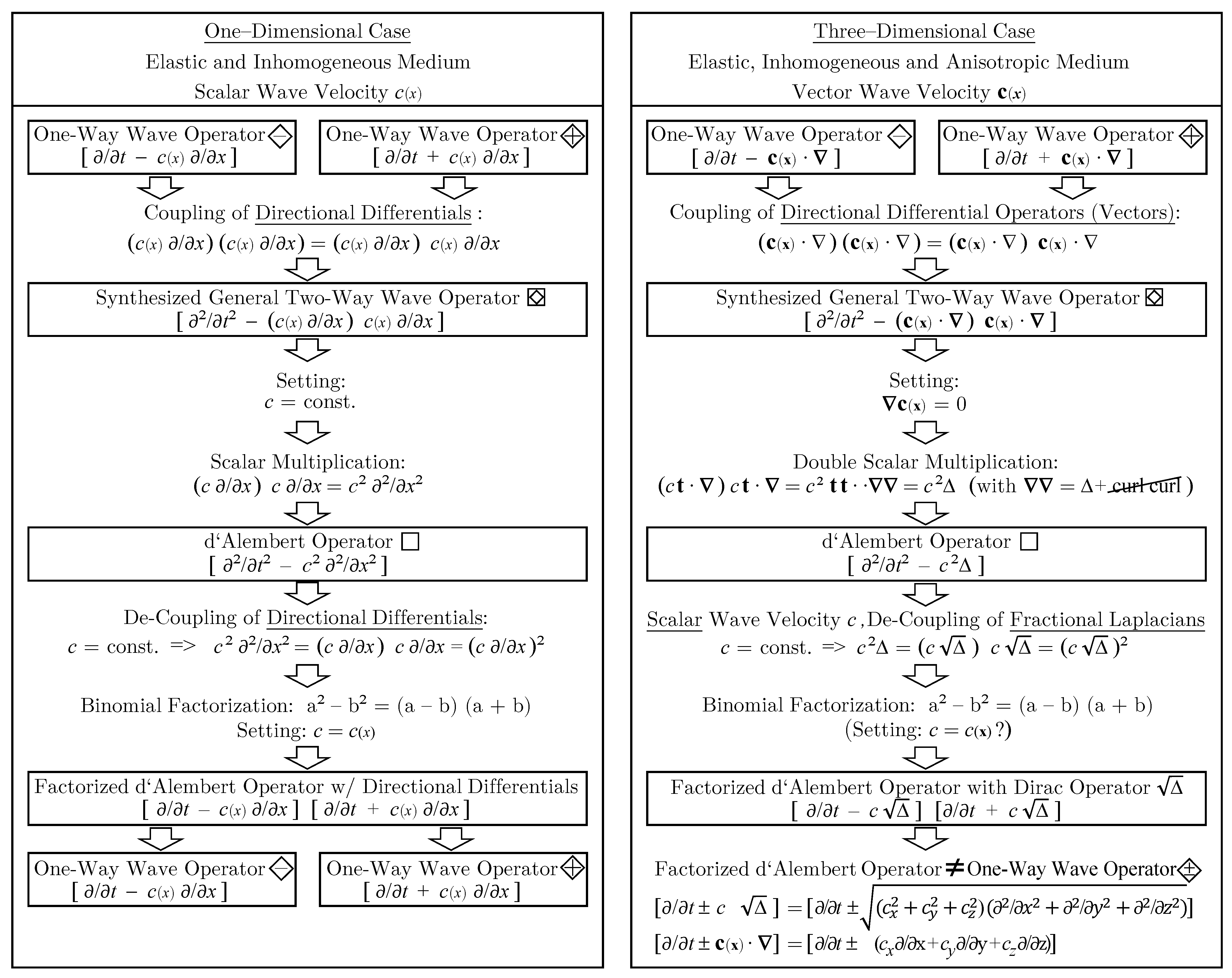
After the spatial one-way/two-way equivalence has been established for longitudinal and transversal waves in the three-dimensional case, the relevant steps of the synthesis and the binomial factorization are compared with the one-dimensional case. As shown in Figure 1, the transformations are similar and require analogous settings of the wave velocity. The comparison also shows that the quantity of the wave velocity (scalar, vector) is crucial.
6. One-Way/Two-Way Equivalence: Other Mechanical and Electromagnetic Waves
The longitudinal and transversal wave equations, often serve as the blueprint for a other wave types [7,11]. The established one-way/two-way equivalence of longitudinal and transversal waves can be transferred to other mechanical and electromagnetic waves. In Table 1, different wave types are listed for plane waves or standing wave fields with constant wave velocity in homogeneous and isotropic media.
Equivalence is established between two coupled one-way wave operators and the two-way d’Alembert wave operator, that are applied to the respective field variables. Beside the governing wave equations also the solutions and the wave velocities are given. The analytical solutions for inhomogeneous or anisotropic media can be determined with the one-way wave equations by stepwise calculation of the pathway.
7. Discussion
For analytical three-dimensional wave (field) calculations the spatial two-way wave equation is commonly taken as the default starting point. As can be seen above, the conventional two-way wave equation is only valid for a constant wave velocity (). Due to this, calculations of wave paths in inhomogeneous or anisotropic media are performed by numerical approximations. However, with one-way wave equations stepwise analytical calculations of wave paths in inhomogeneous or anisotropic media are possible.
The synthesized general vector two-way wave operator also shows that complex standing wave fields can be calculated by simple coupling of one-way wave operators. For complex tasks this is an interesting alternative to the d’Alembert operator approach. To derive the standing wave field solutions, the solutions of the individual one-waves have to be superposed. Boundary conditions can be considered for the single waves.
With the one-way/two-way equivalence for wave fields in homogeneous media, Cauchy’s first equation of motion [2] resulting from Newton’s force equilibrium, see Equation (1), can be also derived from an impulse flow equilibrium by coupling of two one-way operators and performing the double scalar multiplication (requiring ):
Thus, for plane wave propagation in homogeneous media the force-based and the impulse-based approaches lead to expressions that can be converted into each other.
If a two-way wave equation can be factorized, it is an indication that the two-way wave equation is correct. For example, the well-known Webster second-order two-way horn equation for wave propagation in semi-infinite horns can not be factorized. It can be shown, that its validity is limited to conical horns (corresponding to a spherical radiation). It also predicts “artefacts” like an infinite wave velocity at a so-called cut-off frequency [14]. Vice versa, in complex cases it might be easier to find a one-way wave equation and to synthesize the respective two-way wave equation than to physically derive it.
To further investigate and experimentally prove the validity of the one-way theory, precision measurements of wave propagation in inhomogeneous or anisotropic media can be conducted and compared with the results of the analytical one-way predictions and respective numerical approximations based on the two-way theory (if available).
Table 2 compares aspects of the one-way and general/special two-way approaches. Derived by synthesis the general two-way approach has the same solutions as the respective one-way wave equations (without any limitation regarding the vector wave velocity).
The one-way wave equation was hypothetically constituted on the basis of an impulse flow equilibrium [7], but it could also be derived from the impedance theorem [15]. A measurement with a semi-infinite exponential horn [16] confirmed, that waves propagate through at/under the “cut-off frequency” with the local wave velocity, as predicted by the one-way theory. This is in contrast to the “Webster horn equation” predicting a local wave velocity with infinite values at the cut-off frequency and no real wave propagation below cut-off frequency. The PDE factorization of mechanical and electromagnetic wave equations could be achieved as well [11]. The mathematical conversion of two vector one-way wave operators into a vector two-way wave operator and the one-way/two-way equivalence is a mathematical proof of the one-way theory. Table 3 gives a respective overview.
8. Conclusions
The definition of the one-way wave operator symbol ◇ is an important cornerstone for the one-way wave theory. The symbol allows for its analogous usage and representation in formulas, as the d’Alembert operator □ does for the conventional two-way wave theory.
The “synthesis” of two opposite one-way wave operators leads to a synthesized “general two-way wave operator”, and the “general one-way/two-way equivalence” can be established. Instead of solving the general two-way wave equation the solutions of the individual one-way wave equations can be used for the single wave propagation. In case of standing waves the solutions of two one-way wave equations can be superposed taking the respective border conditions or impedances into account for the single waves.
The equivalence with the d’Alembert operator is only possible in the special case of a constant vector wave velocity, because the sequence of two directional differential operators has to be considered. It follows, that for a constant vector wave velocity also the force-based Cauchy’s first equation of motion can be synthesized from two coupled impulse-based one-way wave operators. General and special one-way/two-way equivalences of the wave operators are transferred to other mechanical and electromagnetic wave types.
The comparison of the synthesis with the spatial binomial factorization shows, that factorization does not take into consideration the vector character of the one-way wave operator leading to the mentioned sequence of the directional differential operators. The terms resulting from the factorization do not describe physically propagating waves and also significantly differ from the respective one-way wave operator expressions. The conduction of alternative calculations based on the one-way wave operators and their synthesis potentially improves the understanding of complex wave phenomenas.
The one-way wave operators and the respective one-way wave equations provide mathematical advantages and reduce calculation efforts due to their first-order differentials. The consideration of the vector wave velocity results in unambiguous solutions and allows for the calculation of wave paths in inhomogeneous and/or anisotropic media. The one-way/two-way equivalence provides new insights for science and engineering, and the one-way wave operators may support advanced wave and wave field calculations.
Funding
This research received no external funding.
Data Availability Statement
Not applicable.
Conflicts of Interest
The author declares no conflict of interest.
References
- Garber, E. The Language of Physics, The Calculus and the Development of Theoretical Physics in Europe, 1750–1914; Springer Science & Business Media: New York, NY, USA, 1999. [Google Scholar]
- Truesdell, C.A. Cauchy and the modern mechanics of continua. Rev. D’Histoire Sci. 1992, 45, 22. [Google Scholar] [CrossRef]
- Arfken, G.B.; Weber, H.J.; Harris, F.E. Mathematical Methods for Physicists, 7th ed.; Academic Press: Waltham, MA, USA; Oxford, UK, 2012; pp. 409–413. [Google Scholar]
- Strauss, W. Partial Differential Equations; John Wiley & Sons, Inc.: Hoboken, NJ, USA, 2008; pp. 33–35. [Google Scholar]
- Dirac, P.A.M. The quantum theory of the electron, I,II. Proc R. Soc. Lond. 1928, 117, 610–624. [Google Scholar]
- Lamoureux, M.P. The mathematics of PDEs and the wave equation. In Proceedings of the Seismic Imaging Summer School, University of Calgary, Calgary, AB, Canada, 7–11 August 2006; p. 7. [Google Scholar]
- Bschorr, O. Deviationswellen in Festkörpern. In Proceedings of the DAGA 2014—40th German Annual Conference of Acoustics, Oldenburg, Germany, 10–13 March 2014; pp. 80–81. [Google Scholar]
- Falk, G.; Ruppel, W. Mechanik. Relativität. Gravitation. Die Physik des Naturwissenschaftlers, 3rd ed.; Springer-Verlag: Berlin/Heidelberg, Germany; New York, NY, USA, 1983. [Google Scholar]
- Hermann, F. Skripten zur Experimentalphysik; Universität Karlsruhe: Karlsruhe, Germany, 1997; p. 8. [Google Scholar]
- Bschorr, O.; Raida, H.-J. Transversal One-Way Wave Equation. In Proceedings of the DAGA 2020—45th German Annual Conference of Acoustics, Hannover, Germany, 16–19 March 2020; pp. 1075–1076. [Google Scholar]
- Bschorr, O.; Raida, H.-J. Factorized One-Way Wave Equations. Acoustics 2021, 3, 717–722. [Google Scholar] [CrossRef]
- Lagally, M. Vorlesungen über Vektor-Rechnung; Akademische Verlagsgesellschaft Geest & Portig KG: Leipzig, Germany, 1964; p. 69. [Google Scholar]
- Baysal, E.; Koslo, D.D.; Sherwood, J.W.C. A two-way nonreflecting wave equation. Geophysics 1984, 49, 132–141. [Google Scholar] [CrossRef] [Green Version]
- Bschorr, O.; Raida, H.-J. One-Way Vibration Absorber. Acoustics 2022, 4, 554–563. [Google Scholar] [CrossRef]
- Bschorr, O.; Raida, H.-J. One-Way Wave Equation Derived from Impedance Theorem. Acoustics 2020, 2, 12. [Google Scholar] [CrossRef]
- Raida, H.-J.; Bschorr, O. Konventionelles Kräftegleichgewicht vs hypothetisches Impulsflussgleichgewicht. In Proceedings of the DAGA 2018—44th German Annual Conference of Acoustics, Munich, Germany, 19–22 March 2018; pp. 828–831. [Google Scholar]
Figure 1.
Synthesis of two one-way wave operators and the subsequent binomial factorization. One-dimensional case: The synthesis starts with the multiplication of the one-way operators and their differentials, and the “general two-way wave operator” for the linear case results which respects the sequence of the differentials for a variable wave velocity . A respective wave equation has the same solutions as two one-way wave equations. The setting leads to the d’Alembert operator [13]. With the factorization the operators can be separated, but only for a constant wave velocity due to the sequence of the differentials. Three-dimensional case: The synthesis begins, as in the one-dimensional case, with the multiplication of the one-way operators and their directional differential operators. The spatial “general two-way wave operator” with the specific sequence of operators results. The restriction to or is necessary to perform the double scalar multiplication and derive the d’Alembert operator. Keeping the wave velocity as a scalar quantity, the binomial factorization results in two mathematical terms containing the time derivative and the scalar wave velocity multiplied with the Dirac operator. These terms do not describe propagating physical waves. The individual terms significantly differ from the one-way wave operators due to .

Table 1.
Equivalence between two coupled opposing spatial one-way and two-way wave operators, the general two-way wave equation and the two-way wave equation with the d’Alembert operator being valid (*) for the wave propagation in homogeneous media with or (field variable # = {,,,,}, on basis of the table given in [11]). The one-dimensional wave equations are listed for comparison. The wave solutions are given for plane waves traveling with wave velocity in -direction, i.e., for . The transversal waves oscillate in the and direction. For other wave propagation directions, the orthogonally oscillating directions (, ) can be adjusted accordingly.
 |
Designation: cartesian unit vectors and coordinates , s [m] = vector, scalar elastical displacement; [m/s] = particle velocity; [m/s2] = particle acceleration; [m/s] = vector wave velocity; ω [rad/s] = angular frequency; k [rad/m] = wave number. = amplitude; E [Pa] = elasticity modulus; G [Pa] = shear modulus; ρ [kg/m3] = density; φ [°] = angle; T [N] = tensile stress; h [m] = duct wall thickness; D [m] = duct diameter; m [kg/m] = mass distribution per meter; EJ [Pa m4] = bending stiffness; U [V] = electrical voltage; I [A] = electric current; E [V/m] = electric field strength; H [A/m] = magnetic field strength; C [As/Vm] = capacity per unit length; L [Vs/Am] = inductivity per unit length; ϵ [As/Vm] = dielectricity constant; μ [Vs/Am] = permeability constant.
Table 2.
Spatial one-way/two-way approaches, longitudinal (, omitted).
| One-Way | “General” Two-Way | “Special” Two-Way () | |
|---|---|---|---|
| Wave operator |  | ||
| Wave equation |  | ||
| Physical concept | impulse flow equilibrium | 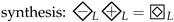 | force equilibrium |
| Wave equation type | 1st order PDE | 2nd order PDE | 2nd order PDE |
| Wave velocity quantity | vector | vector | scalar |
| Wave velocity gradient | possible | possible | (homogeneous media only) |
| Local wave velocity | can be non-local (→ “artefact”) | ||
| Inhomogeneous media | analytical solution | ← use “One-Way” solution | numerical approximation |
| Anisotropic media | analytical solution | ← use “One-Way” solution | numerical approximation |
| Standing wave field | yes (superposition) | ← use “One-Way” solution | yes |
| Unique solutions | yes | ← use “One-Way” solution | ambigous: |
| Mathematical complexity | low | high | high |
| Computation efforts/time | low | high | high |
Table 3.
Derivation of one-way wave equation; proof by alternative derivation, measurement etc.
| Physical Approach | Result |
|---|---|
| Impulse flow equilibrium [7] | tensor one-way wave equation: |
| Derivation from impedance [15] | scalar one-way wave equation: (; ; ; ) |
| Exponential horn measurement [16] | one-way predictions confirmed; no cut-off frequency ; for |
| PDE factorization [11] | one-way wave equations derived for mechanical and electromagnetic waves |
| One-way/two-way equivalence | conversion of spatial one-way wave operators into two-way wave operator, d’Alembertian |
Publisher’s Note: MDPI stays neutral with regard to jurisdictional claims in published maps and institutional affiliations. |
© 2022 by the author. Licensee MDPI, Basel, Switzerland. This article is an open access article distributed under the terms and conditions of the Creative Commons Attribution (CC BY) license (https://creativecommons.org/licenses/by/4.0/).
Share and Cite
MDPI and ACS Style
Raida, H.-J. One-Way Wave Operator. Acoustics 2022, 4, 885-893. https://doi.org/10.3390/acoustics4040053
AMA Style
Raida H-J. One-Way Wave Operator. Acoustics. 2022; 4(4):885-893. https://doi.org/10.3390/acoustics4040053
Chicago/Turabian StyleRaida, Hans-Joachim. 2022. "One-Way Wave Operator" Acoustics 4, no. 4: 885-893. https://doi.org/10.3390/acoustics4040053