The available conventional fatigue model for assessing the corrosion fatigue failures of magnesium mount structural castings is not quite accurate, as the formation of corrosion pits is random in nature and the empirical equations derived from specimen samples are largely in a linear format [
1,
2]. Generally, casting shrinkage and porosity in as-cast magnesium alloys can especially act as stress concentration sites for fatigue crack initiation. In addition to the typical aging issue, oxide inclusions are induced under corrosive environmental conditions. These preferential sites for fatigue crack initiation are related to the formation of pits on the surface, particularly at tensile fiber stress locations. When a magnesium mount structural casting is exposed to a corrosive environment, both anodic and cathodic reactions are happening, with the resulting released hydrogen gas playing a major role in environmental assisted cracking [
1,
2,
3,
4].
Magnesium dissolution in an aqueous solution is an anodic reaction, whilst hydrogen evolution is a cathodic reaction. Hydrogen could diffuse into the magnesium matrix through corrosion pit formation and then cause hydrogen embrittlement, which could significantly reduce the mechanical strength of magnesium alloys. Thus, although the size of the pits is smaller than that of oxide inclusions on fracture surfaces, fatigue cracks can still preferentially nucleate at pits, even at the lower stress amplitude in a NaCl solution than in air.
2.1. Fatigue Life of Magnesium Structural Casting Model for Corrosion
The difference in the fatigue life of magnesium structural casting materials with and without corrosive environmental conditions has been assessed via the available literature to create a material database for assessing field-related technical variances, as also reported in available internal sources [
1,
2,
3].
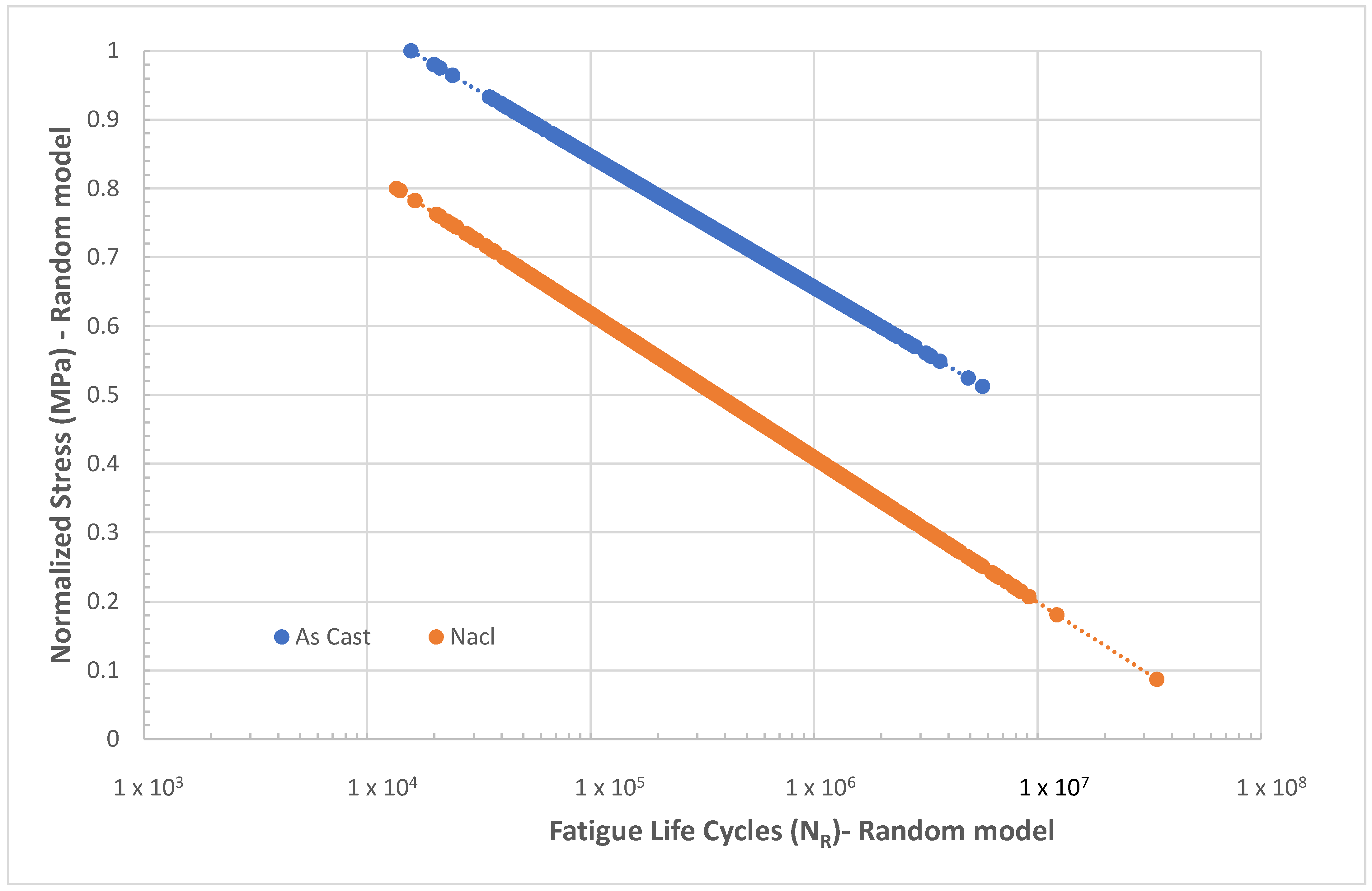
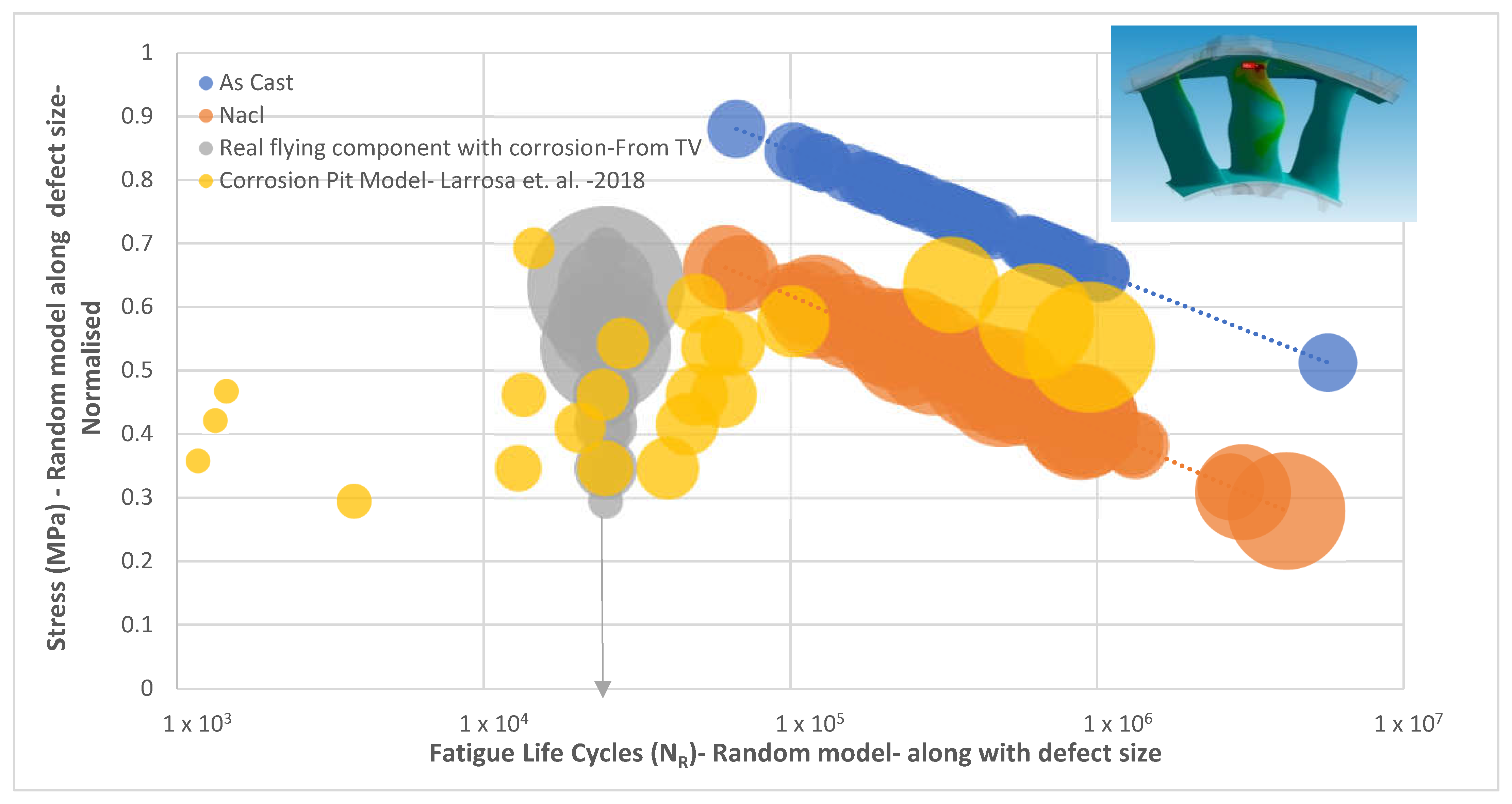
The fatigue life of the as-cast and NaCl solution exposed to a magnesium structure is shown in
Figure 3, taken from Reference [
1], along with the defect sizes, which vary from a minimum of 0.18 mm to a maximum of 7.4 mm in equivalent spherical diameter.
Figure 3 also shows internal Rolls Royce material data for a magnesium cast structure without any corrosion defects (as-cast condition), which coincides with the lower range of fatigue life reported in some cases [
1,
2]. This fatigue strength over a corrosive environmental condition generally can also be degraded over time, which is not considered here for simplification purposes.
The empirical relationship of the corrosion fatigue life of a magnesium structural casting could be obtained from this available experimental data. This fatigue life information is for finite corrosion pit data and has some limitations on being applied directly in solving the field corrosion pit issue for magnesium structural castings. There is a need for an efficient model that addresses the random nature of fatigue, corrosion (pit), and load scenarios. Otherwise, the industry is left only with a rational approach, which is inefficient sometimes. The following section proposes a stochastic corrosion fatigue model.
2.2. Stochastic Process and Random Variable Formulation
In order to explain the problem quantitatively and investigate the regularities of the random phenomenon, it is common practice to introduce a mathematical formulation that brings the randomness together with an appropriate measure of the possibilities of occurrences of various uncertain outcomes of an experiment. Such a model forms a basic system for a probability model in which the main notions are defined as follows:
Sample space: This is defined as the collection of all possible outcomes from the experiments.
Random event: An event that can happen in an unpredictable way.
Probability: The probability of the event.
The sample space is denoted as Ω, which contains all the possible or elementary outcomes of an observation denoted as γ, which satisfies γ ∈ Ω. Let ξ be denoted as the family of subsets of Ω, described as the family of random events with which the probability of event P is defined. The probability of event P is described here as the probability of reaching the required fatigue life at a critical porosity fraction. The probability of event P is a function whose arguments are random events that are an element of ξ, so that it follows the following three axioms of modern probability [
2,
3]:
It is clear that in experiments on random phenomena, various outcomes or elementary events can occur. In many situations, they are represented by the real number X (γ). It is also possible that a real number can be assigned to each elementary event; γ ∈ Ω. X(γ) is called a random variable, which is defined as a real-valued function X = X(γ), γ ∈ Ω, defined on the sample space Ω, such that for every real number ‘x’, the probability is defined as
The existence of the probability of event {γ: X (γ) ≤ x} ensures that the probability of any finite or countable infinite combination of such events is well defined as P {x1 < X (γ) ≤ x2}.
The probabilistic behavior of a random variable X (γ) is completely and uniquely specified by the cumulative distribution function F
X (x), which is defined as
By definition, the distribution function always exists and is a non-negative and non-decreasing function of the real variable ‘x’.
Property 1. From the property’s cumulative distribution function, it follows that Property 2. For any two real numbers a, b such that a < b, the probability is computed as Property 3. The function fX (x) is non-negative. Integrating the density function on an event gives us the probability of the event. This property can be proved easily since the probability density function is the derivative of the cumulative distribution function. As this cumulative function is a non-decreasing function, its derivative can never be negative.
2.2.1. Single Random Variables: Formulations
The basic probability model for a single random variable is defined in this section.
Assume that a random variable X (γ) is termed as a continuous random variable if its probability distribution function F
X (x) has a density function, such that
where ‘U’ is defined as any dummy variable. The function f
X (x) is called the probability density function of the random variable X (γ). Hence,
Further properties of probability density function are
Physically, when the random samples are drawn from the sample space Ω, it is essential to compute the mean and standard deviation of these random samples so that the probability density function could be derived based on the type of distribution function it follows. When the random samples are repeated ‘N’ times, by having the X as random variables and x as real set numbers, among N experiments, the real value x
i can be repeated as n
i times, and the average or mean is calculated as
Intuitively, the quantity of
is none other than measuring the probability of obtaining the result x
i over N experiments. Then, Equation (9) can be re-written as
N is random samples, which are infinitely growing, and X is the random variable, which is sometimes equal to the real number x
i; the ratio
goes to an infinitesimally small quantity, which represents f
x(x
i). dx at point x
i. The mean or average value of a random variable is defined as an operator called the expectation operator, E(X).
The notation E (.) stands for the average value operator, commonly called a mathematical expectation. Equation (11) is a similitude of the center of gravity equation, which is defined as a summation of the product of each area strip to the length of the strips divided by the total area of the body. The denominator of Equation (11) represents the total area of the probability density function, which is unity. Hence, Equation (11) becomes
Equation (12) is also called the average or mean value of the random variables X (γ), which is denoted as μX.
The variance of random variables X(γ) is defined as
The square root of Equation (13) is called the standard deviation of the random variables.
The ratio of variance to mean provides a coefficient of variation, which normalizes the spread of occurrence of real numbers from the random variables X(γ).
Ideally, Equation (15) represents the standard deviation of random variables, which is the difference between the mean square value and the square of the mean of random variables. Physically, σX measures the dispersion of the experimental results around its average value. When σX is small, the probability density function of X is a curve concentrated around its mean. When σX is large, this curve flattens and gets wider.
By the same means, the moments of any order n can be introduced:
and the order ‘n’ centered moments are formulated by
The characteristic function is an important analytical tool that enables us to analyze the sum of independent random variables. Moreover, this function contains all the necessary information specific to the random variables X.
2.2.2. Bivariate and Multivariate Random Variables: Formulations
The basic probability model when there are two or more random variables is defined in this section by the above description, which is based on a single random variable. This means it is also possible to generalize the above equations for the multi-dimensional case. It is focused now instead of on random variables to on random vectors.
Let X be a two-dimensional random vector X = (X
1, X
2). The joint cumulative distribution function of the random variables X
1 and X
2 are also called the cumulative distribution function of the random vector X, which is defined as being similar to Equations (1) and (4).
Defined directly from the probability of axioms, single random variables are alternatively changed as
0 ≤ P {x1 ≤ X (γ) ≤ x2} ≤ 1, for each A∈ ξ;
P(Ω) = 1, or FX1, X2 (+∞, +∞) = 1;
FX1, X2 (x1, −∞) = 0 and FX1, X2 ( −∞, x2) = 0;
For any countable collection of mutually disjoint events, A1, A2, … An in ξ:
As with the case of a single random variable, in the vector case, it is necessary to build a function called the joint probability density function of the variables X
1 and X
2 such that with the integration of these two events in the sample space, the conditional probability is obtained as
It is now essential to bring the basic fundamental properties of the conditional probability of events, which gives
The condition for Equation (22) is that X1 and X2 are independent random variables, and then the joint probability density function of the two independent random variables is given by the product of their respective marginal densities.
Similarly, the mean, variance, moments, and centered order of moments are also defined for bivariate random variables.
The joint moments of order n and m for the X
1 and X
2 random variables are
The centered ordered n, m moments are
Among the centered moments, the most important parameter is called covariance between the two random variables X1 and X2.
Equation (27) is called the variance–covariance matrix of the (X1, X2) vector. If these two random variables are independent of each other, then their covariance is zero. If their correlation value is zero, then these variables are said to be orthogonal.
The correlation coefficient between the two random variables X
1, and X
2 is calculated as
For the transformation of n-dimensional random vectors, the Jacobian matrix of coordinates mapping is used. The stochastic equation, which may be used to describe the time-dependent corrosion process, should consist of two main parameters that describe the fluctuation in environmental conditions and the microscopical structural behavior of the material. The correlation of the microscopic mechanisms of corrosion with its macroscopic statistical nature is needed for the development of a stochastic corrosion fatigue equation. The macroscopic mechanisms of the corrosion of the material can be derived by referencing the empirical equation from experiments. The microscopical structural behavior of the material can be determined with two factors: the consideration of fluctuations in the environment and the average background of the structure superimposed by inhomogeneous fluctuations due to a variety of inherent defects.
The stochastic equation is used to describe the process of corrosion, as presented in the above stochastic process with a random variable as the pit formation with respect to fatigue life and stress (loading). Because fluctuations in the environment or the microscopic structure led to stochastic variations in the corrosion rate, it should obey the above-mentioned stochastic corrosion fatigue model along with the experimentally obtained empirical equations (as presented in the next section).


