A Stochastic Corrosion Fatigue Model for Assessing the Airworthiness of the Front Flanges of Fleet Aero Engines Using an Automated Data Analysis Method

Abstract

Corrosion, combined with cyclic loading, is inevitable and becomes a challenging problem, even when inherently corrosion-protected materials have been selected and applied based on established in-house experience. Aero engine mount structures are exposed to dusty and salty environmental conditions during both operational and non-operational periods. It is becoming tough to predict the remaining useful corrosion fatigue life due to the unascertainable material strength degradations under service conditions. As such, a rationalized approach is currently being used to assess their structural integrity, which produces more wastages of the flying parts. This paper presents a novel approach for predicting corrosion fatigue by proposing a random-parameter model in combination with validated experimental data. The two-random-parameter model is employed here with the probability method to determine the time-independent corrosion fatigue life of a magnesium structural casting, which is used heavily in engine front-mount aircraft systems. This is also correlated with experimental data from the literature, validating the proposed stochastic corrosion fatigue model that addresses the technical variances that occur during service to increase optimal mount structure usage using an automated data system.

1. Introduction

Magnesium structural castings are potential candidate materials for applications in automobile and aerospace industries due to their abundant availability and low cost. However, in real service conditions, the structural components often suffer from corrosive attack due to exposure to harsh environments, aggravating magnesium structural casting aging. There are many previous studies on magnesium structural castings and their fatigue corrosion strength [1,2]. However, accurate models that predict the fatigue life of magnesium structural castings in corrosive environments are still limited [1]. In the aerospace industry, in particular, static components of aero engines manufactured from magnesium cast alloys are sometimes evaluated conservatively to maintain their airworthiness during service. Magnesium structural castings are more prone to corrosive attack, along with operational fatigue load, compared to other structural castings [3]. Building a corrosion fatigue model for the on-wing condition of aircraft engine structural components is crucial and in demand, as this would help to optimize effective fleet planning. Additionally, it could also mean reducing engine maintenance and consequently decreasing costs. For every flight from January 2012 to December 2020, most of the environmental contaminants that aggravated corrosive attack were salt, sand, dust, SO₂, and SO₄, which, due to the lack of a corrosion fatigue model, incurred a loss of approximately GBP 7.5 million worth of damage [2,4,5,6]. With data quenching through internal flight information facts for a contamination model with actual flight cycles, compared with other conditions’ effects on corrosion fatigue failure mode, a salty environment is the worst in deteriorating the structural integrity of static engine components. The severity of environmental salt exposure for Rolls Royce engines with various operators can be observed in Figure 1 compared to dusty conditions (different-colored lines indicate different airlines) [2].

There are also numerous aspects that need to be addressed in terms of technical variance during regular and frequent maintenance visits for magnesium structural casting-based aero engine mount components. Out of all of these technical variances gathered over the last eight years, 27% are based on corrosion in structural castings for one engine type program. Of these, 18% are based on corrosion fatigue issues and have a magnesium structural casting as an intermediate structure, as shown in Figure 2.

The current paper aims to provide a novel stochastic corrosion fatigue model for assessing these technical variances in a quantitative manner to optimize the remaining useful life period of structural castings; it overcomes the conventional approaches—such as rationalization, pragmatic analysis, and qualified methods—by limiting damage size (corrosion pits) so that the scrapping of the engine mount structure can be better controlled in robust way.

2. Corrosion Fatigue Model

The available conventional fatigue model for assessing the corrosion fatigue failures of magnesium mount structural castings is not quite accurate, as the formation of corrosion pits is random in nature and the empirical equations derived from specimen samples are largely in a linear format [1,2]. Generally, casting shrinkage and porosity in as-cast magnesium alloys can especially act as stress concentration sites for fatigue crack initiation. In addition to the typical aging issue, oxide inclusions are induced under corrosive environmental conditions. These preferential sites for fatigue crack initiation are related to the formation of pits on the surface, particularly at tensile fiber stress locations. When a magnesium mount structural casting is exposed to a corrosive environment, both anodic and cathodic reactions are happening, with the resulting released hydrogen gas playing a major role in environmental assisted cracking [1,2,3,4].

Magnesium dissolution in an aqueous solution is an anodic reaction, whilst hydrogen evolution is a cathodic reaction. Hydrogen could diffuse into the magnesium matrix through corrosion pit formation and then cause hydrogen embrittlement, which could significantly reduce the mechanical strength of magnesium alloys. Thus, although the size of the pits is smaller than that of oxide inclusions on fracture surfaces, fatigue cracks can still preferentially nucleate at pits, even at the lower stress amplitude in a NaCl solution than in air.

2.1. Fatigue Life of Magnesium Structural Casting Model for Corrosion

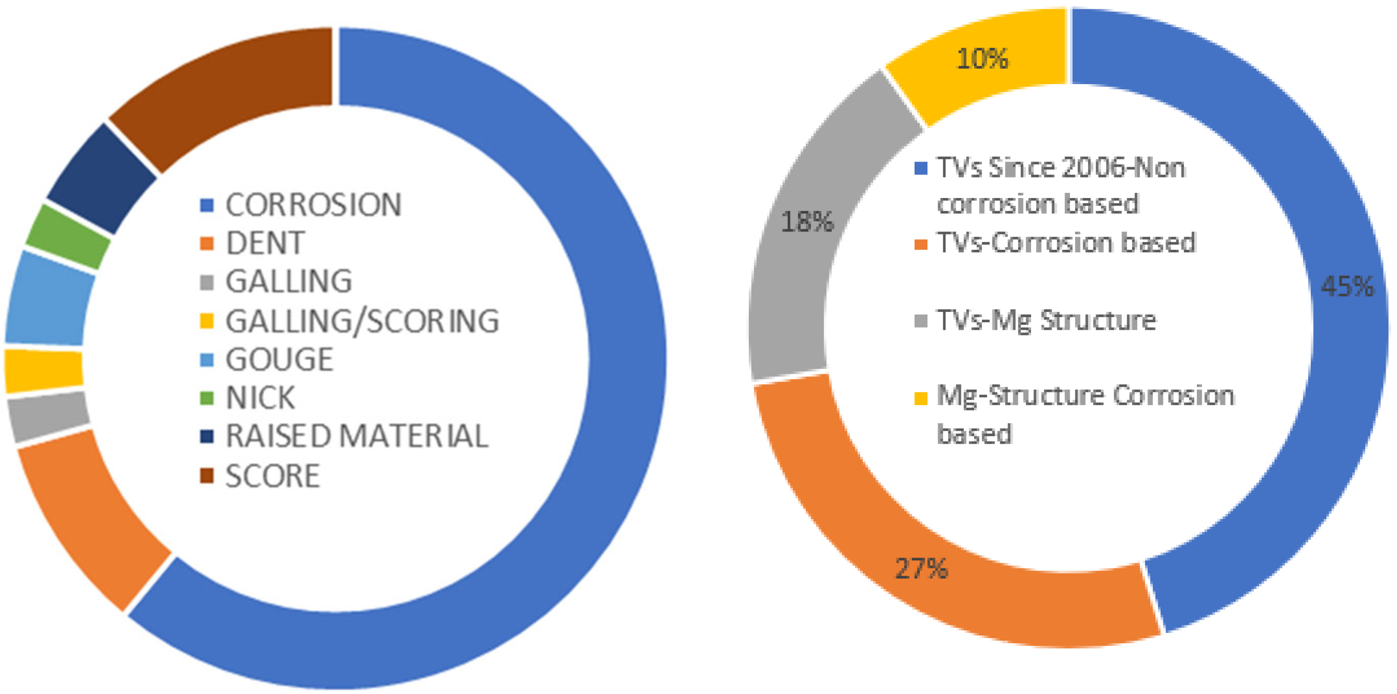
The difference in the fatigue life of magnesium structural casting materials with and without corrosive environmental conditions has been assessed via the available literature to create a material database for assessing field-related technical variances, as also reported in available internal sources [1,2,3].

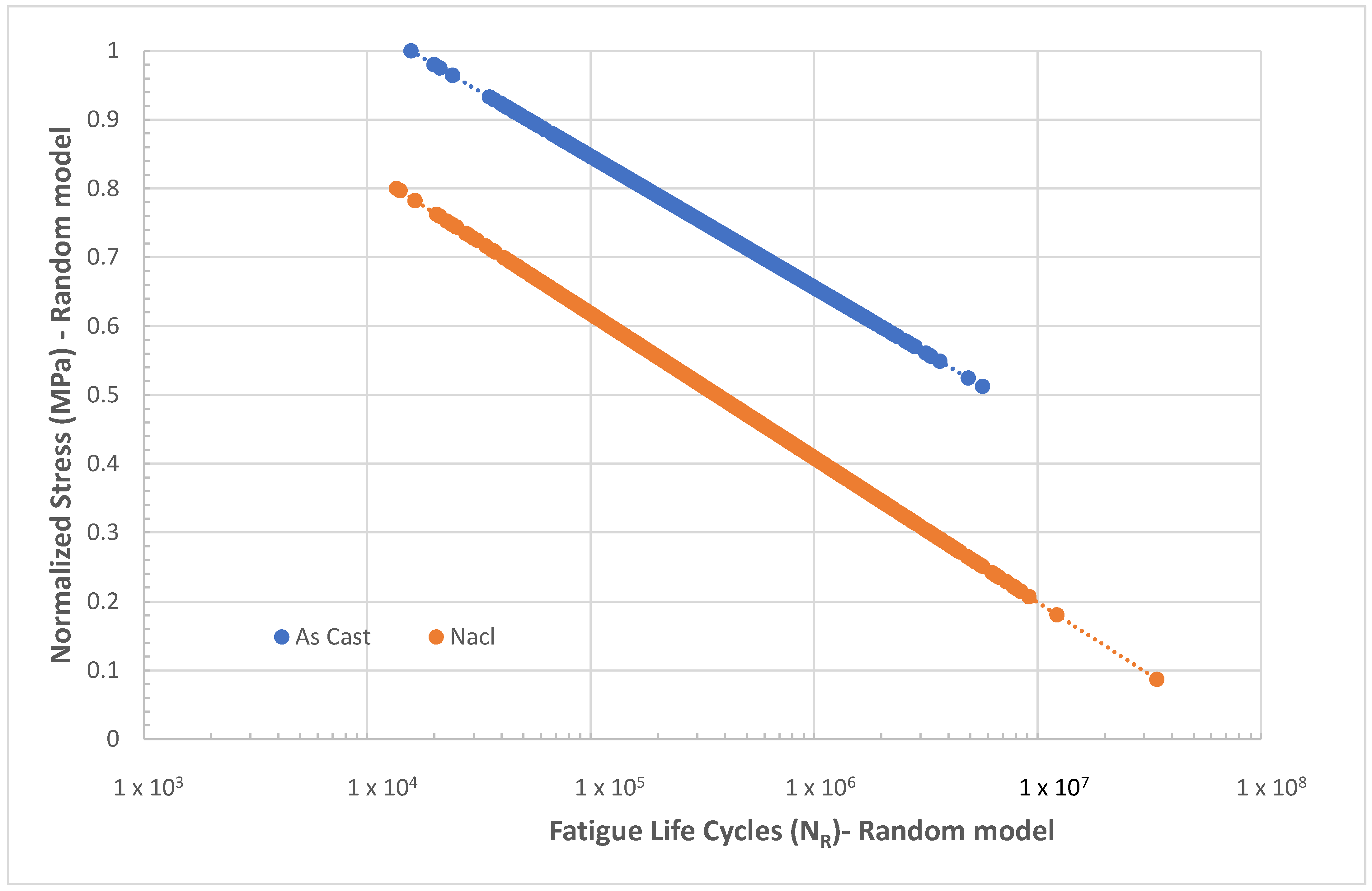
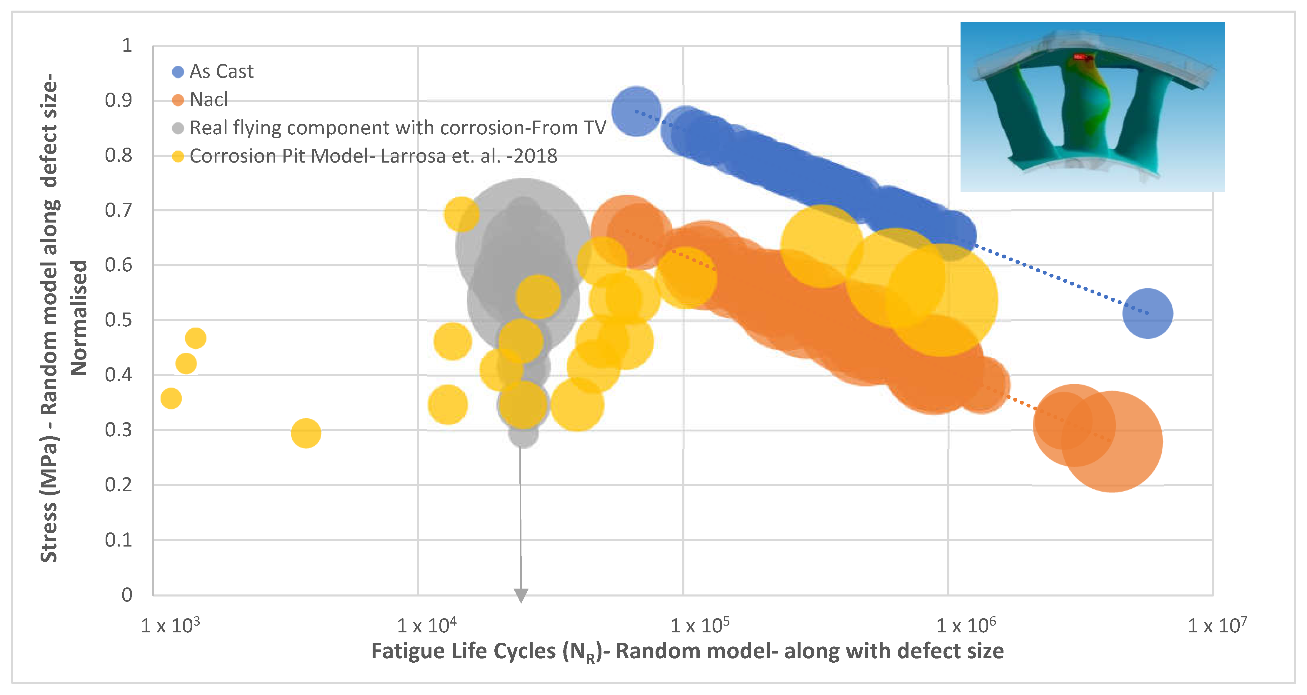
The fatigue life of the as-cast and NaCl solution exposed to a magnesium structure is shown in Figure 3, taken from Reference [1], along with the defect sizes, which vary from a minimum of 0.18 mm to a maximum of 7.4 mm in equivalent spherical diameter. Figure 3 also shows internal Rolls Royce material data for a magnesium cast structure without any corrosion defects (as-cast condition), which coincides with the lower range of fatigue life reported in some cases [1,2]. This fatigue strength over a corrosive environmental condition generally can also be degraded over time, which is not considered here for simplification purposes.

The empirical relationship of the corrosion fatigue life of a magnesium structural casting could be obtained from this available experimental data. This fatigue life information is for finite corrosion pit data and has some limitations on being applied directly in solving the field corrosion pit issue for magnesium structural castings. There is a need for an efficient model that addresses the random nature of fatigue, corrosion (pit), and load scenarios. Otherwise, the industry is left only with a rational approach, which is inefficient sometimes. The following section proposes a stochastic corrosion fatigue model.

2.2. Stochastic Process and Random Variable Formulation

In order to explain the problem quantitatively and investigate the regularities of the random phenomenon, it is common practice to introduce a mathematical formulation that brings the randomness together with an appropriate measure of the possibilities of occurrences of various uncertain outcomes of an experiment. Such a model forms a basic system for a probability model in which the main notions are defined as follows:

Sample space: This is defined as the collection of all possible outcomes from the experiments.

Random event: An event that can happen in an unpredictable way.

Probability: The probability of the event.

The sample space is denoted as Ω, which contains all the possible or elementary outcomes of an observation denoted as γ, which satisfies γ ∈ Ω. Let ξ be denoted as the family of subsets of Ω, described as the family of random events with which the probability of event P is defined. The probability of event P is described here as the probability of reaching the required fatigue life at a critical porosity fraction. The probability of event P is a function whose arguments are random events that are an element of ξ, so that it follows the following three axioms of modern probability [2,3]:

• 0 ≤ P(A) ≤ 1, for each A ∈ ξ.
• P(Ω) = 1.
• For any countable collection of mutually disjoint events, A₁, A₂, … A_n in ξ:

  P{ ∪ A_n} = Σ P(A_n)

It is clear that in experiments on random phenomena, various outcomes or elementary events can occur. In many situations, they are represented by the real number X (γ). It is also possible that a real number can be assigned to each elementary event; γ ∈ Ω. X(γ) is called a random variable, which is defined as a real-valued function X = X(γ), γ ∈ Ω, defined on the sample space Ω, such that for every real number ‘x’, the probability is defined as

P{Ω: X(γ) ≤ x }

The existence of the probability of event {γ: X (γ) ≤ x} ensures that the probability of any finite or countable infinite combination of such events is well defined as P {x₁ < X (γ) ≤ x₂}.

The probabilistic behavior of a random variable X (γ) is completely and uniquely specified by the cumulative distribution function F_X (x), which is defined as

F_X (x) = P {X (γ) ≤ x}

(1)

By definition, the distribution function always exists and is a non-negative and non-decreasing function of the real variable ‘x’.

Property 1. 

From the property’s cumulative distribution function, it follows that

F_X (−∞) = 0; and F_X (+∞) = 1

(2)

Property 2. 

For any two real numbers a, b such that a < b, the probability is computed as

P {a < X ≤ b) = F_X (b) − F_X (a).

(3)

Property 3. 

The function f_X (x) is non-negative. Integrating the density function on an event gives us the probability of the event. This property can be proved easily since the probability density function is the derivative of the cumulative distribution function. As this cumulative function is a non-decreasing function, its derivative can never be negative.

2.2.1. Single Random Variables: Formulations

The basic probability model for a single random variable is defined in this section.

Assume that a random variable X (γ) is termed as a continuous random variable if its probability distribution function F_X (x) has a density function, such that

$$F_X\left(x\right)={\int }_{-\infty }^x{f}_x\left(U\right).dU$$

(4)

where ‘U’ is defined as any dummy variable. The function f_X (x) is called the probability density function of the random variable X (γ). Hence,

$${\displaystyle \frac{d{F}_X\left(x\right)}{dx}}=f_X\left(x\right)$$

(5)

Further properties of probability density function are

$$f_X\left(x\right)\ge 0$$

(6)

$${\int }_a^b{f}_X\left(x\right)dx=F_X\left(b\right)-F_X\left(a\right)$$

(7)

$${\int }_{-\infty }^{+\infty }f\left(x\right)dx=1$$

(8)

Physically, when the random samples are drawn from the sample space Ω, it is essential to compute the mean and standard deviation of these random samples so that the probability density function could be derived based on the type of distribution function it follows. When the random samples are repeated ‘N’ times, by having the X as random variables and x as real set numbers, among N experiments, the real value x_i can be repeated as n_i times, and the average or mean is calculated as

$$\overline{X}={\sum }_{i=1}^N\left({\displaystyle \frac{n_i}{N}}\right)x_i$$

(9)

Intuitively, the quantity of ${\displaystyle \frac{n_i}{N}}$ is none other than measuring the probability of obtaining the result x_i over N experiments. Then, Equation (9) can be re-written as

$$\overline{X}={\sum }_{i=1}^N{x}_i.P\left(X=x_i\right)$$

(10)

N is random samples, which are infinitely growing, and X is the random variable, which is sometimes equal to the real number x_i; the ratio ${\displaystyle \frac{n_i}{N}}$ goes to an infinitesimally small quantity, which represents f_x(x_i). dx at point x_i. The mean or average value of a random variable is defined as an operator called the expectation operator, E(X).

$$E\left[X\right]={\displaystyle \frac{{\int }_{-\infty }^{+\infty }X.f_X\left(x\right)dx}{{\int }_{-\infty }^{+\infty }{f}_X\left(x\right)dx}}$$

(11)

The notation E (.) stands for the average value operator, commonly called a mathematical expectation. Equation (11) is a similitude of the center of gravity equation, which is defined as a summation of the product of each area strip to the length of the strips divided by the total area of the body. The denominator of Equation (11) represents the total area of the probability density function, which is unity. Hence, Equation (11) becomes

$$E\left[X\right]={\int }_{-\infty }^{+\infty }X. f_X\left(x\right)dx$$

(12)

Equation (12) is also called the average or mean value of the random variables X (γ), which is denoted as μ_X.

The variance of random variables X(γ) is defined as

$$E\left[{\left(X-{\mu }_X\right)}^2\right]={\int }_{-\infty }^{+\infty }{\left(X-{\mu }_X\right)}^2.f_X\left(x\right)dx$$

(13)

The square root of Equation (13) is called the standard deviation of the random variables.

$${\sigma }_X^2=E\left[{\left(X-{\mu }_X\right)}^2\right]={\int }_{-\infty }^{+\infty }{\left(X-{\mu }_X\right)}^2.f_X\left(x\right)dx$$

(14)

$${\sigma }_X^2=E\left[X^2\right]-{\mu }_X^2$$

(15)

The ratio of variance to mean provides a coefficient of variation, which normalizes the spread of occurrence of real numbers from the random variables X(γ).

Ideally, Equation (15) represents the standard deviation of random variables, which is the difference between the mean square value and the square of the mean of random variables. Physically, σ_X measures the dispersion of the experimental results around its average value. When σ_X is small, the probability density function of X is a curve concentrated around its mean. When σ_X is large, this curve flattens and gets wider.

By the same means, the moments of any order n can be introduced:

$$M_X^n=E\left[X^n\right]={\int }_{-\infty }^{+\infty }{X}^n{f}_X\left(x\right)dx$$

(16)

and the order ‘n’ centered moments are formulated by

$$C_X^n=E\left[{\left(X-{\mu }_X\right)}^n\right]={\int }_{-\mathrm{\infty }}^{+\mathrm{\infty }}{\left(X-{\mu }_X\right)}^n{f}_X\left(x\right)dx$$

(17)

The characteristic function is an important analytical tool that enables us to analyze the sum of independent random variables. Moreover, this function contains all the necessary information specific to the random variables X.

2.2.2. Bivariate and Multivariate Random Variables: Formulations

The basic probability model when there are two or more random variables is defined in this section by the above description, which is based on a single random variable. This means it is also possible to generalize the above equations for the multi-dimensional case. It is focused now instead of on random variables to on random vectors.

Let X be a two-dimensional random vector X = (X₁, X₂). The joint cumulative distribution function of the random variables X₁ and X₂ are also called the cumulative distribution function of the random vector X, which is defined as being similar to Equations (1) and (4).

F_{X1, X2} (x₁, x₂) = P {x₁ ≤ X (γ) ≤ x₂}

(18)

Defined directly from the probability of axioms, single random variables are alternatively changed as

• 0 ≤ P {x₁ ≤ X (γ) ≤ x₂} ≤ 1, for each A∈ ξ;
• P(Ω) = 1, or F_{X1, X2} (+∞, +∞) = 1;
• F_{X1, X2} (x₁, −∞) = 0 and F_{X1, X2} ( −∞, x₂) = 0;
• For any countable collection of mutually disjoint events, A₁, A₂, … A_n in ξ:

P{ ∪ A_n} = Σ P(A_n)

As with the case of a single random variable, in the vector case, it is necessary to build a function called the joint probability density function of the variables X₁ and X₂ such that with the integration of these two events in the sample space, the conditional probability is obtained as

$$\begin{array}{cc}{F}_{X1, X2}\left(x_1,x_2\right)=\hfill & \iint f_{X1, X2}\left(x_1,x_2\right)d{x}_{1}d{x}_2\hfill \\ & =P(\left\{x_1<X_1\le x_1+d{x}_1 and x_2<X_2\le x_2+d{x}_2\right\}\hfill \end{array}$$

(19)

This also allows

$$f_{X1,X2}\left(x_1,x_2\right)={\displaystyle \frac{{\partial }^2{F}_{X1,X2}\left(x_1,x_2\right)}{\partial x_1\partial x_2}}$$

(20)

$$F_{X1, X2}\left(x_1,x_2\right)={\int }_{-\infty }^{x_1}{\int }_{-\infty }^{x_2}{f}_{X1, X2}\left(u,v\right)dudv$$

(21)

It is now essential to bring the basic fundamental properties of the conditional probability of events, which gives

$$f_{X1, X2}\left(x_1,x_2\right)=f_{X1 }\left(x_1\right).f_{X2 }\left(x_2\right)$$

(22)

The condition for Equation (22) is that X₁ and X₂ are independent random variables, and then the joint probability density function of the two independent random variables is given by the product of their respective marginal densities.

Similarly, the mean, variance, moments, and centered order of moments are also defined for bivariate random variables.

$$E\left[X\right]={\int }_{-\infty }^{+\infty }{\int }_{-\infty }^{+\infty }{X.f}_{X1, X2}\left(u,v\right)du.dv$$

(23)

$${\sigma }_X^2=E\left[{\left(X-{\mu }_X\right)}^2\right]={\int }_{-\infty }^{+\infty }{\left(X-{\mu }_X\right)}^2.f_{X1, X2}\left(u,v\right)du.dv$$

(24)

The joint moments of order n and m for the X₁ and X₂ random variables are

$$M_{X1, X2}^{n,m}=E\left[X_1^n{X}_2^m\right]={\int }_{-\infty }^{+\infty }{\int }_{-\infty }^{+\infty } X_1^n{X}_2^m{f}_{X1, X2}\left(u,v\right)du.dv$$

(25)

The centered ordered n, m moments are

$$\begin{array}{c}{C}_{X1, X2}^{n,m}=E\left[{\left(X_1-{\mu }_X\right)}^n{\left(X_2-{\mu }_X\right)}^m\right] \hfill \\ ={\int }_{-\infty }^{+\infty }{\int }_{-\infty }^{+\infty } {\left(X_1-{\mu }_{X1}\right)}^n{{\left(X_2-{\mu }_{X2}\right)}^{m}f}_{X1, X2}\left(u,v\right)du.dv\hfill \end{array}$$

(26)

Among the centered moments, the most important parameter $C_{X_1{X}_2}^{\mathrm{1,1}}$ is called covariance between the two random variables X₁ and X₂.

The matrix is

$$\left[\begin{array}{cc}{C}_{X_1{X}_1}^{\mathrm{1,1}}& C_{X_1{X}_2}^{\mathrm{1,1}}\\ C_{X_2{X}_1}^{\mathrm{1,1}}& C_{X_2{X}_2}^{\mathrm{1,1}}\end{array}\right]$$

(27)

Equation (27) is called the variance–covariance matrix of the (X₁, X₂) vector. If these two random variables are independent of each other, then their covariance is zero. If their correlation value is zero, then these variables are said to be orthogonal.

The correlation coefficient between the two random variables X₁, and X₂ is calculated as

$$\rho ={\displaystyle \frac{C_{X_1{X}_2}^{\mathrm{1,1}}}{{\sigma }_{X_1}{\sigma }_{X_2}}}$$

(28)

For the transformation of n-dimensional random vectors, the Jacobian matrix of coordinates mapping is used. The stochastic equation, which may be used to describe the time-dependent corrosion process, should consist of two main parameters that describe the fluctuation in environmental conditions and the microscopical structural behavior of the material. The correlation of the microscopic mechanisms of corrosion with its macroscopic statistical nature is needed for the development of a stochastic corrosion fatigue equation. The macroscopic mechanisms of the corrosion of the material can be derived by referencing the empirical equation from experiments. The microscopical structural behavior of the material can be determined with two factors: the consideration of fluctuations in the environment and the average background of the structure superimposed by inhomogeneous fluctuations due to a variety of inherent defects.

The stochastic equation is used to describe the process of corrosion, as presented in the above stochastic process with a random variable as the pit formation with respect to fatigue life and stress (loading). Because fluctuations in the environment or the microscopic structure led to stochastic variations in the corrosion rate, it should obey the above-mentioned stochastic corrosion fatigue model along with the experimentally obtained empirical equations (as presented in the next section).

2.3. Stochastic Corrosion Fatigue (SCF) Model

Let the stress amplitude (S_a) have a cumulative density function (CDF) of F_Sa; then, the lifetime size of corrosion pits (N*C_P) has a CDF of F_NCP, and the relationship between these two CDFs is established for NaCl as

$${\mathrm{F}}_{{\mathrm{S}}_{\mathrm{a}}}={\mathrm{F}}_{\mathrm{N}{\mathrm{C}}_{\mathrm{P}}}{\left({\displaystyle \frac{{\mathrm{S}}_{\mathrm{a}}}{1062.1}}\right)}^{1/-0.197}$$

(29)

The probability distribution function is derived from the above equation by

$${\mathrm{f}}_{{\mathrm{S}}_{\mathrm{a}}}={\displaystyle \frac{\mathrm{d}}{\mathrm{d}\mathrm{x}}}\left({\mathrm{F}}_{{\mathrm{S}}_{\mathrm{a}}}\right)$$

(30)

The mean and variance have also been formulated for each dependent and independent random variable [2].

$$\mathrm{E}\left[{\mathrm{S}}_{\mathrm{a}}\right]=1062.1\ast \mathrm{E}{\left[\mathrm{N}\right]}^{-0.197}\ast \mathrm{E}{\left[{\mathrm{C}}_{\mathrm{P}}\right]}^{-0.197}$$

(31)

$${\mathsf{\mu }}_{{\mathrm{S}}_{\mathrm{a}}}=1062.1\ast {\mathsf{\mu }}_{\mathrm{N}}^{-0.197}\ast {\mathsf{\mu }}_{{\mathrm{C}}_{\mathrm{P}}}^{-0.197}$$

(32)

$${\mathsf{\sigma }}_{{\mathrm{S}}_{\mathrm{a}}}^2={1062.1}^2\ast \left[{\mathsf{\sigma }}_{\mathrm{N}{\mathrm{C}}_{\mathrm{P}}}^2\right]$$

(33)

Now, with the available probabilistic parameters and based on the Monte Carlo random model technique, the range of experimental parameters is sampled 1000 times, as is shown in Figure 4.

3. Implementation of SCF Model to Technical Variances

If the grain boundary near the free surface is not very well protected by an oxide layer, oxygen gas or other embrittling species may diffuse along the boundary and react with grain boundary precipitates [1]. Under this influential condition of loads, stress spikes at the cavities are present around the grain boundary precipitates, which are accelerated by repeated environmental exposure of the structures during their services.

A combination of surface diffusion and slip step oxidation promotes the enhanced kinematic irreversibility of cyclic slip that causes earlier fatigue cracks to nucleate in the absence of other mechanisms. This step is also accelerated by porosities and voids in magnesium structural casting.

Preferential oxidation at certain microstructural sites, such as at the intersection of a grain boundary with a free surface, causes microscopic stress concentrations (notches) to develop. The micro-notches elevate the local stresses and promote crack nucleation. The expected high-stress profile features are also identified for these structures, and, based on field experience, the identified stress corrosion features are assessed for their corrosion fatigue life to avoid any premature failures.

The fleet reported corrosion fatigue defects and corresponding fatigue life to be cleared for the required life mission, and at the experienced fatigue loading conditions, the reported technical variances are assessed based on the proposed stochastic fatigue model for corrosion (SFC), as is shown in Figure 5, instead of any qualitative-based assessment, which is the conventional method that has usually been followed.

Commonly, the evaluation of these issues regarding the technical variance of corrosion on magnesium structural castings is carried out based on individual assessment with a rational qualitative basis. This proposed SCF model will bring not only a new concept with a quantitative approach, but also the remaining useful life period is calculated more effectively based on the evidence collected with experimental data.

Figure 5 gives the real flying fleet corrosive data within the specification of the randomly generated fatigue life of known corrosive defects that was calculated with the proposed stochastic corrosive fatigue model with a normalized stress plot of the engine support structure. Since it has been cleared for the required number of flight cycles, the real-world corrosion-attacked components are at a constant life curve but with various bubble sizes that indicate the corrosion sizes with varying fatigue strength. The analytical corrosion model that has been derived out in Appendix A, shows also good correlations in comparison with experiments as well as proposed stochastic corrosion fatigue model.

The following results were obtained from the presented stochastic corrosion fatigue model with actual fleet data of an aero engine of front flanges raised for technical variances.

Figure 6 provides the real raw data of corrosion pit size that was observed from the fleet (relevant to Figure 2 of internal TV database) with a probability distribution plot along with two different distribution functions to be compared. Figure 7 uses the largest extreme value distribution functions to generate random numbers within the defined stochastic model, as proposed in an earlier section for assessing the fleet corrosion problems of front-mount flange Mg structural castings. In this way, Figure 7 categorizes the acceptance limits and ranges within an operational scope in automatically designed data.

Figure 6 and Figure 7 provide the real-time quantitative data analysis set from the SCF model on magnesium structural casting in actual fleet engine data, which not only saves time and costs but also provides a robust model for the calculation of remaining useful life. The arrows indicate the current requirements for the airworthiness of the part.

4. Conclusions

In this study, corrosion from real field experiments due to service issues on a magnesium structural casting of an engine mount critical structure was analyzed and assessed based on available qualitative assessment methods, which resulted in rejection of the part despite it having potential for a longer period of usage. This was challenged and addressed by proposing a real-time automated data analysis system that was proposed based on a stochastic corrosion fatigue model. This model was developed and validated based on corrosion-related fatigue data from the literature as well as from in-house material data sets. This paper brings not only a novel approach to predicting corrosion fatigue by proposing a random-parameter model in combination with experimental data but also effectively solves the two-random-parameter model with the probability method to determine the time-independent corrosion fatigue life of magnesium structural castings used heavily in mount structures. The same is also correlated with experimental data from the literature for validating the proposed stochastic corrosion fatigue model to address the technical variance that occurs while the part is in service. In the future, this model can be improved by implementing time-dependent parameters for corrosion pit formation along with a real-time simulation of pits due to corrosion fatigue.

References

1. Wang, S.D.; Xu, D.K.; Wang, B.J.; Han, E.H.; Dong, C. Effect of corrosion attack on the fatigue behaviour of an as-cast Mg-7%Gd-5%Y-1%Nd-0.5%Zr alloy. Mater. Des. 2015, 84, 185–193. [Google Scholar] [CrossRef]
2. Narayanan, G. Probabilistic fatigue model for cast alloys of aero engine applications. Int. J. Struct. Integr. 2021, 12, 454–469. [Google Scholar] [CrossRef]
3. Haiyun, H. Stochastic theory of fatigue corrosion. Phys. Lett. A 1999, 261, 217–225. [Google Scholar] [CrossRef]
4. Urbano, J.; Golowin, A.; Löhnert, S.; Bestle, D. Mechanical Integrity of Steel Discs with Corrosion Pits. MATEC Web Conf. 2018, 165, 04012. [Google Scholar] [CrossRef]
5. Larrosa, N.; Akid, R. Corrosion Fatigue: A review of damage tolerance models. Int. Mater. Rev. 2018, 63, 283–308. [Google Scholar] [CrossRef]
6. Mao, M.; Zhang, X.; Tu, S.; Xuan, F. Prediction of crack initiation life due to corrosion pits. J. Aircr. 2014, 51, 805–810. [Google Scholar] [CrossRef]
7. Ishihara, S.; Saka, S.; Nan, Z.Y. Prediction of corrosion fatigue lives of aluminium alloy on the basis of corrosion pit growth law. Fatigue Fract. Eng. Mater. Struct. 2006, 29, 472–480. [Google Scholar] [CrossRef]
Figure 1. Amount of total contamination by dust (above) and salt exposure (below) in aero engines over cycles for different airline operators over the past eight years.
Cmd 06 00032 g001
Figure 2. Technical variances of corrosion problems and related magnesium casting support structure.
Cmd 06 00032 g002
Figure 3. Stress–life curve for as-cast versus NaCl-exposed Mg cast alloy [1].
Cmd 06 00032 g003
Figure 4. Stress–life curve for as-cast versus NaCl-exposed Mg cast alloy from random model with experimental raw data (#1000 random samples).
Cmd 06 00032 g004
Figure 5. Fleet technical variance of corrosive fatigue loading condition of engine intermediate magnesium cast structure along with SFC model [5].
Cmd 06 00032 g005
Figure 6. Real data set for Mg corrosion pit formation from fleet data of engine intermediate magnesium cast structure along with SFC model.
Cmd 06 00032 g006aCmd 06 00032 g006b
Figure 7. Stochastic corrosion fatigue model assessment on fleet technical variance based on proposed automated quantitative data analysis method for airworthiness purposes.
Cmd 06 00032 g007aCmd 06 00032 g007b
Disclaimer/Publisher’s Note: The statements, opinions and data contained in all publications are solely those of the individual author(s) and contributor(s) and not of MDPI and/or the editor(s). MDPI and/or the editor(s) disclaim responsibility for any injury to people or property resulting from any ideas, methods, instructions or products referred to in the content.