Article

Stochastic Analysis of Electron Transfer and Mass Transport in Confined Solid/Liquid Interfaces

Helmholtz-Zentrum Berlin für Materialien und Energie GmbH, Institute for Solar Fuels, Hahn-Meitner-Platz 1, D-14109 Berlin, Germany
Surfaces 2020, 3(3), 392-407; https://doi.org/10.3390/surfaces3030029
Submission received: 6 July 2020 / Revised: 3 August 2020 / Accepted: 5 August 2020 / Published: 8 August 2020

Abstract

:
Molecular-level understanding of electrified solid/liquid interfaces has recently been enabled thanks to the development of novel in situ/operando spectroscopic tools. Among those, ambient pressure photoelectron spectroscopy performed in the tender/hard X-ray region and coupled with the “dip and pull” method makes it possible to simultaneously interrogate the chemical composition of the interface and built-in electrical potentials. On the other hand, only thin liquid films (on the order of tens of nanometers at most) can be investigated, since the photo-emitted electrons must travel through the electrolyte layer to reach the photoelectron analyzer. Due to the challenging control and stability of nm-thick liquid films, a detailed experimental electrochemical investigation of such thin electrolyte layers is still lacking. This work therefore aims at characterizing the electrochemical behavior of solid/liquid interfaces when confined in nanometer-sized regions using a stochastic simulation approach. The investigation was performed by modeling (i) the electron transfer between a solid surface and a one-electron redox couple and (ii) its diffusion in solution. Our findings show that the well-known thin-layer voltammetry theory elaborated by Hubbard can be successfully applied to describe the voltammetric behavior of such nanometer-sized interfaces. We also provide an estimation of the current densities developed in these confined interfaces, resulting in values on the order of few hundreds of nA·cm−2. We believe that our results can contribute to the comprehension of the physical/chemical properties of nano-interfaces, thereby aiding to a better understanding of the capabilities and limitations of the “dip and pull” method.

Graphical Abstract

1. Introduction

The development of in situ/operando characterization tools aiming to directly probe solid/liquid interfaces [1,2,3,4,5,6,7,8] has greatly advanced our comprehension of molecular-level processes occurring at these interfaces, such as specific adsorption of ions, charge transfer dynamics and electrical (Galvani) potential formation. Several spectroscopic methods based on photon in/photon out and photon in/electron out approaches have been developed and successfully applied to investigate electrified solid/liquid interfaces. In recent years, ambient pressure X-ray photoelectron spectroscopy (AP-XPS) has proven to be a powerful in situ characterization technique, since it offers elemental and chemical sensitivity, while simultaneously making it possible to measure local built-in electrical potentials under realistic working conditions [9,10,11,12,13,14,15,16,17,18]. The extension of AP-XPS to high photon energies (and, therefore, high photoelectron KEs) [7,8,9,10,11,12,13,14,15,16,17,19] is particularly suited for investigating solid/liquid interfaces. First, the reduced scattering of high-energy photoelectrons by gas molecules provides detectable signal intensity at relatively high gas pressures, up to and beyond the vapor pressure of water at room temperature (~25 mbar). Second, photoelectrons with a KE between 2000 and 10,000 eV have an inelastic mean free path (IMFP) in water between approximately 5 and 20 nm, enabling the investigation of solid/liquid junctions through electrolyte layers with thicknesses on the same order as the IMFP [7,8,9].
The key factor for investigating solid/liquid interfaces using electron detection is therefore the preparation of (stable) liquid films thick enough to be representative of a realistic interface, but thin enough to allow photoelectrons ejected from the interfacial region to penetrate and emerge from the liquid on their path to the photoelectron analyzer [7]. Currently, two different preparation and investigation approaches are used, which differ from each other by the side of the interface through which the X-ray incidence and electron detection are performed [20]. In the first approach, the latter are carried out on the “solid side” of the junction using membranes composed of few graphene layers supporting the solid phase, the latter typically in the form of finely dispersed nanoparticles [21,22,23,24]. This method offers the great advantage of allowing gases or liquids to flow through the system, thereby providing facile mass transport. The disadvantage is that only thin solid films can be investigated since the photo-emitted electrons must travel through the solid phase/graphene membrane to reach the photoelectron analyzer [7]. In the second approach, the X-ray incidence and electron detection are instead conducted on the “liquid side” of the solid/liquid interface. This requires the preparation of a thin liquid layer atop the solid surface [20]. This method allows investigating a broader range of solid materials of arbitrary thickness, and it is, therefore, particularly important for photoelectrochemical (PEC) interfaces, where the thickness of the semiconducting photoanode/cathode must match the diffusion length of the photo excited charge carriers (typically spanning from tens to hundreds of nm). In addition, such approach is applicable to fundamental investigations of interfaces such as the simultaneous probing of the electrical potential distribution within the solid (i.e., band-bending) and the liquid side of the junction (the double/diffuse layer) [11,15,25].
The preparation of liquid layers characterized by a thickness on the order of few tens of nanometer that are stable for the duration of the measurements (often several hours) is not straightforward. So far, three experimental procedures have been developed to obtain such “free-surface” liquid layers [7]: the “emersion technique” (known also as ‘’dip and pull”) [9,26,27,28,29], “the tilted sample” procedure [30], and the “offset droplet” method [31]. These techniques, widely used within the AP-XPS community, share, however, two limitations: first, they can only be used with solid samples characterized by wettable surfaces. More specifically, the contact angle ψ at the liquid meniscus must be smaller than 90° (thus indicating relatively intense interactions between the solid and the liquid). Second, the mass transport in the liquid along the direction parallel to the solid surface is severely limited in these thin liquid films, which limits the electrochemical current densities that can be reached during the in situ experiments [7,32,33]. Therefore, due to the described limitations and the corresponding experimental challenges (e.g., control and stability of nm-thick liquid layers), a detailed experimental electrochemical investigation of such thin electrolyte layers is still lacking.
This work therefore aims at characterizing the electrochemical behavior of solid/liquid interfaces in confined spaces, where the diffusion of reactants is limited to the direction orthogonal to the interface. The investigation has been performed using a stochastic modeling of (i) the electron transfer (ET) between a solid surface and a one-electron redox couple and (ii) its diffusion in solution. The simulations, carried out using the freely available Kinetiscope program package [34], were performed for both non-confined and confined geometries in order to provide a benchmark for our simulations and therefore to highlight the true electrochemical properties of nano-sized interfaces. The voltammetric response of such confined interfaces was investigated in terms of the electrolyte layer thickness, the standard reaction rate, the potential scan rate, and the transfer coefficient. Our findings show that the electrochemical behavior of these “confined interfaces” can be described in terms of the well-known thin-layer voltammetry theory elaborated by Hubbard [35], due to the mass transport limitations along the direction parallel to the solid/liquid interface. Therefore, we find that the electrochemical current is not limited by the diffusion of reactants, but is instead controlled by the reaction rate itself at the electrode. We also provide an estimation of the current densities developed in such confined spaces, resulting on the order of few hundreds of nA·cm−2 at most. In particular, and in agreement with the Hubbard’s model, we find that the current density is a linear function of the thickness of the liquid layer atop the solid surface. Our findings are general and valid for one-electron redox couples in both aqueous and non-aqueous media.
We believe that our results can contribute to the comprehension of the true physical/chemical properties of solid/liquid interfaces where the liquid side is characterized by thicknesses of few tens of nanometers.

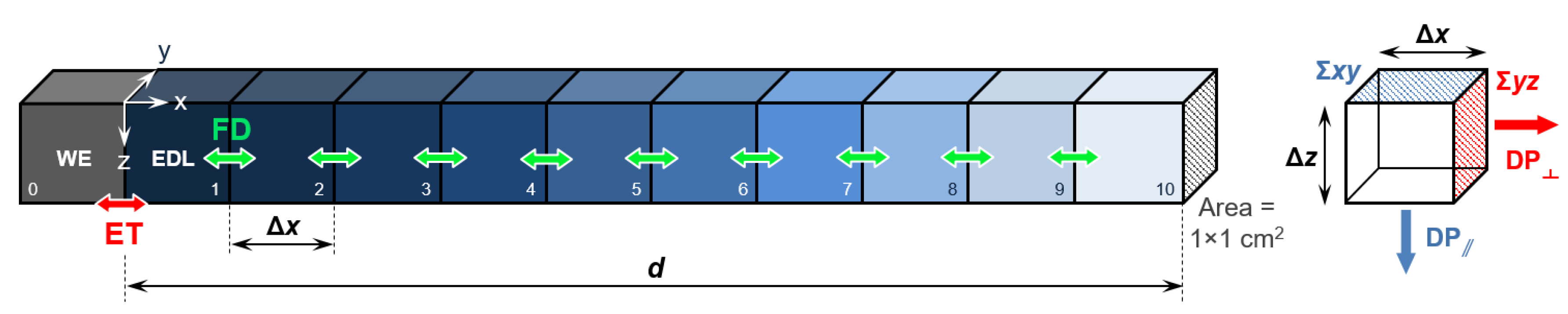
2. Methods: Stochastic Simulation Details

The stochastic simulations reported in this work were generated using the freely available Kinetiscope program package, developed by F.A. Houle and W.D. Hinsberg [34]. Merging and extending the previous numerical codes CKS and VSIM [34,36,37], Kinetiscope makes it possible to treat the electron transfer (ET) and the Fick diffusion (FD) at the molecular level via a random walk through the reaction event space, instead using the more typical approach involving deterministic-coupled differential equations. This approach was therefore chosen to carry out the simulations reported in this work because it is particularly useful to simulate small volumes (as it is the case with confined liquids) containing a small number of molecules [38]. An extensive description of the software and tutorials explaining how to simulate different reactive environments (including the “three dimensional scheme with electrochemistry” example) can be found on the web page [34] and in refs. [36,37,39].
The simulated electrochemical medium was a solution at room temperature (r.t., 298 K) containing a symmetric monovalent supporting electrolyte (e.g., C+A) at a concentration (ionic strength, I) of 0.1 M (0.1 mol·L−1). Under these conditions, the Debye length (k−1) for the electrolyte (describing the electrostatic screening of the charges in solution) can be calculated as follows (Equation (1)) [40]:
k−1 = [εr·ε0·RT/(2 × 103·F2·I)]½
εr and ε0 are the relative and vacuum (8.854 × 10⁻¹² F·m−1) dielectric permittivity, respectively. F and R are the Faraday constant (9.64853 × 10⁴ C·mol−1) and the molar gas constant (8.31447 J·mol−1·K−1), respectively. T is the temperature (in K). For a 0.1 M aqueous solution at r.t (εr water = 80.2 [41]), k−1 = 0.96 nm. The quantity 3·k−1 (2.88 nm), which is the distance in the solution at which the electrostatic potential due to the charged electrode is reduced to 5% of its value at the electrode surface, can be thereby taken as the thickness of the electrical double layer (EDL). Within the Gouy–Chapman–Stern model [40], the definition of the EDL given in this study comprises the Stern and the diffuse layer. Please note that within this definition, the thickness of the EDL is also equivalent to the separation at which the electrostatic interaction between the charge density at the electrode surface and an elementary charge is comparable in magnitude to the thermal energy, kBT (equal to about 25.7 meV (4.12 × 10⁻²¹ J) at r.t.).
The simulations in Kinetiscope were carried out as schematically reported in Figure 1, with the solid/liquid interface parametrized as discrete square volume elements [34] with surface area of 1 × 1 cm2. The first element (0) is the working electrode (WE). The elements from 1 to 10 represent the electrolyte solution atop the electrode surface, with element 1 simulating the EDL.
The simulated molecular probe was a one-electron redox couple with a diffusion coefficient D at r.t. equal to 0.5 × 10⁻⁵ cm2·s−1 for both the oxidized and reduced species. The redox couple obeys the following electrochemical equilibrium at zero overpotential (i.e., at E°) (Equation (2)):
O + e R
O and R indicate the oxidized and reduced species in solution, respectively.
For the “bulk interface” simulations, the liquid element size perpendicular to the electrode surface exponentially expands from 2.88 × 10⁻⁷ cm (2.88 nm) for the element 1 to 1.0 × 10⁻¹ cm for the element 10. The total thickness of the liquid electrolyte d was therefore equal to 1320 µm. This value was chosen to ensure that the liquid layer thickness was larger than the diffusion layer thickness l for all the investigated potential sweep ranges (either in the anodic or cathodic direction starting from the equilibrium potential E° of the redox couple) and scan rates. The values of l for all the different simulated conditions are reported in Table 1, and have been determined using the following relation (Equation (3)) [38]:
l = 6·(D·Δt)½
For the “confined interface” simulations, we investigated three electrolyte layer thicknesses (d): 10, 20, and 30 nm. These values are in line with the typical values achieved experimentally when performing “dip and pull” measurements [7,8,9,10,11,12,13,14,15,19,20]. In this case, the Δx dimensions of liquid elements 2–10 were identical and set at a fixed value for the different liquid layer thicknesses simulated in this work (Table 2).
As reported in Figure 1, two transfer paths were then introduced between the liquid elements: the ET path between the WE (element 0) and the redox couple present in the element 1 (EDL) and the FD path between the different liquid elements (1–10). The stochastic simulations were then performed by setting the voltammetric pattern and following the solute concentration and current flowing through the WE as a function of time. The simulations of the “bulk” (and “confined”) interfaces were performed setting the number of Monte Carlo trajectories to 1 × 10⁸ (and 1 × 10⁵, respectively).
The electrochemical kinetics of the ET path were implemented in Kinetiscope using the Butler–Volmer model. The relation between the current density flowing through the electrode at the time t and the overpotential between the latter and the bulk electrolyte has the following form (Equation (4)) [38]:
J (x = 0, t) = Fk0·[CO (x = 0, texp [−αηF/RT] − CR(x = 0, t)·exp [(1 − α) ηF/RT]
k0 is the standard rate constant (in cm·s−1). The transfer coefficient α (which is a dimensionless number) represents a measure of the symmetry of the reaction energy barrier (ΔG). For α = ½ the barrier is symmetric. For 0 ≤ α < ½ the activated complex (or transition state) is closer to the product R, whereas when ½ > α ≥ 1 the activated complex is closer to the reagents O + e [42].
η is the overpotential (in V), while CO(0,t) and CR(0,t) are the concentrations (in mol·L−1) of the oxidized and reduced species at the electrode surface (x = 0) at the time t. The simulations were performed setting a concentration of 0.5 mM at x = 0 for both the reduced R and oxidized O species, at the equilibrium potential of the redox couple E° at t = 0. The total concentration of the redox couple in solution at each time t of the simulation was therefore equal to 1.0 mM. Different values and combinations of k0 and α were investigated, as described in the “Results and Discussion” section.
Let us now describe how the diffusion of the redox couple was treated in the stochastic simulations. It is possible to identify two diffusional pathways (DP): parallel (DP, along the z direction in Figure 1) and orthogonal to the sample surface (DP⫠, along the x direction in Figure 1). It should be realized, however, that the time scale for the diffusion along the DP path is some orders of magnitude longer compared to that for the DP⫠ path, and therefore it can be ignored. To demonstrate that, we use Fick’s first law of diffusion (Equation (5)) [38]:
J (x, y, z) = n/(Σ·∆t) = −D·∇C(x, y, z)
where J represents the diffusional flux, which is the number of moles of redox couple (n) contained in a volume V that flows through the liquid layer cross-section (Σ) within the time ∆t. ∇C(x, y, z) is the concentration gradient in the solution that drives the diffusion. After rearrangement, Equation (5) leads to the following expression for the diffusional time scale (Equation (6)), where the concentration gradient is approximated to its finite difference along the x, y, or z direction:
t = |n/Σ·1/D·[∇C(x, y, z)]−1| ~ |n/Σ·1/D·[ΔC(x, y, z)x, y, z]−1|
For the calculation, we take into account a liquid layer thickness d and a lateral dimension of the electrode of 30 × 10−7 cm (30 nm) and 1.0 cm, respectively. Therefore, n = 3 × 10⁻¹² mol (for a redox couple concentration C of 1.0 mM = 1 × 10⁻⁶ mol·cm3), and the electrolyte layer cross-section Σxy (Σyz) on the xy (yz) plane is equal to 30 × 10−7 cm × 1.0 cm = 3 × 10⁻⁶ cm2 (1.0 cm × 1.0 cm = 1.0 cm2). We then define ∆t (∆t⫠) as the time needed to completely deplete the redox couple in the liquid layer having DP (DP⫠) as the only active diffusion pathway (Δz = 1 cm and Δx = 30 × 10−7 cm, respectively, see Figure 1). We found values for ∆t and ∆t⫠ of 2 × 10⁵ s and 1.8 × 10⁻⁶ s, respectively, thereby justifying the choice of considering the DP⫠ as the only active pathway for the redox couple diffusion in solution during the simulations.
The diffusion of the redox couple along the direction x between the liquid elements (DP⫠) was modeled using the Fick’s second law (Equation (7)), which describes how diffusion causes the concentration of the solutes to change with respect to time under the assumption of mass conservation (absence of chemical reactions in solution) [38]:
∂CO,R(x, t)/∂t = D·∂2CO,R(x, t)/∂x2
For each investigated set of parameters, we simulated cyclic voltammograms (CVs) with the initial and final potential fixed at η = 0.0 V (i.e., at the equilibrium potential of the redox couple, E°), acquiring a current value every 0.1 s. The initial concentration of the oxidized (O) and reduced species (R) in solution was set to 0.5 mM, for a total concentration of the redox couple equal to 1.0 mM.
To benchmark the outputs obtained for the “confined interface”, we also simulated the voltammetric response of a conventional “bulk interface” (d = 1320 µm) under the application of the overpotential with different scan rates. The results for a symmetric (α = 0.5), reversible ET process (k0 = 1.0 cm·s−1) are reported in Figure 2a. The anodic and cathodic peaks, exhibiting a typical asymmetric line shape, do not shift by varying the scan rate as expected from a purely reversible ET. This is also confirmed by the peak-to-peak separation (Δpp) equal to 59.16 ± 0.25 mV, in agreement with the separation expected at r.t. (T = 298 K) for one electron, Nernstian-reversible ET (ln10·RT/F ≈ 2.303·RT/F = 59.13 mV) [43]. The anodic (cathodic) current density at the peak maxima (minima) is proportional to the square root of the scan rate v, as reported in Figure 2b, and in line with the Randles–Sevcik equation for planar, semi-infinite diffusion conditions (Equation (8)) [38]:
jpA,C = 0.4463·(F3/RT)½·D½·C(x = 0)O,R·v½
Figure 2c reports the simulated CVs for a symmetric (α = 0.5), non-reversible ET (k0 = 1.0 × 107 cm·s−1) as a function of the potential scan rate. In contrast to the fast ET, the Δpp between the anodic and cathodic branch of the cyclic voltammetry increases by increasing the scan rate, with the Δpp significantly exceeding the quantity 2.303·RT/F = 59.13 mV as expected from an irreversible redox couple (Δpp passes from 545 mV at a scan rate of 25 mV·s−1 to 650 mV at 200 mV·s−1). Additionally, in this case, the simulations are in agreement with the experimental results [44,45], showing that the anodic and cathodic peak currents obey Equation (8) as well (Figure 2d).

3. Results and Discussion

Now that the simulation methodology has been validated, we proceed to characterize the voltammetric response of the “confined interface”. For this, we use the well-known thin film voltammetry theory outlined by A. T. Hubbard in 1969 [35]. Our aim was to verify whether this model, which has been successfully used to describe electrochemical systems with liquid film thicknesses spannig from tens to hundreds of μm [35,43,46], can also be used to qualitatively and quantitatively describe nanometer-sized interfaces. We start by briefly summarizing the main points and equations of Hubbard’s model.
First of all, to help discriminating between the “bulk” and “confined” regimes, and to remove the dependency from the choice of the electrolyte layer thickness and potential scan rate, we introduce the “Hubbard number” H. This is defined as the ratio between the electrolyte layer thickness and the potential scan rate (Hd/v). For instance, for the simulations reported in Figure 2 (with d = 1320 µm), H went from 5.28 cm·V−1·s at a scan rate of 25 mV·s−1 to 0.66 cm·V−1·s at 200 mV·s−1. For the simulations of a “confined interface” with d = 30 nm, H ranges instead from 1.2 × 10⁻⁴ cm·V−1·s at a scan rate of 25 mV·s−1 to 1.5 × 10⁻⁵ cm·V−1·s at 200 mV·s−1.
If H ≤ 0.5 cm·V−1·s, Equation (8) does not hold and must be substituted by the Hubbard relations. For a reversible (k0 >> 4 × 10⁻³ cm·s−1 [35]) monoelectronic ET, the oxidation and reduction peaks are centered at the equilibrium potential of the redox couple (η = 0), and are characterized by a full-width at half-maximum (FWHM) equal to 3.530·RT/F = 90.6 mV at r.t. (T = 298 K) [43]. The peak current density jp is found to be linearly dependent on the thickness of the liquid layer (d), the concentration of reactants at the electrode surface (C(x = 0)O,R), and the potential scan rate (v) [35] (Equation (9)):
jpA,CRev = ± ¼·F2/(RTd·C(x = 0)O,R·v
Notably, the Hubbard’s model predicts that for an irreversible monoelectronic ET the peak current density jp depends also on the transfer coefficient α (Equation (10)):
jpA,CIrr = ± α/2.718·F2/(RTd·C(x = 0)O,R·v
This is of particular interest for fundamental investigations of electrochemical reactions, since it makes it possible to access to the symmetry of the reagent and product free energy curves around the reaction energy barrier. For an irreversible ET, the potential at which the oxidation and reduction peaks are centered shifts according to Equation (11):
ηp A,CIrr = ± RT/(αF)·ln [(RTk0)/(αFdv)]
Note that Equation (11) holds when k0 ≤ 1.0 × 105 cm·s1 and ηp C,A ≥ 100 mV [35].
Taking our cue from Hubbard’s findings, we conducted a series of stochastic simulations where the “confined interface” was investigated in terms of the electrolyte layer thickness d, the standard reaction rate k0, the potential scan rate v, and the transfer coefficient α.

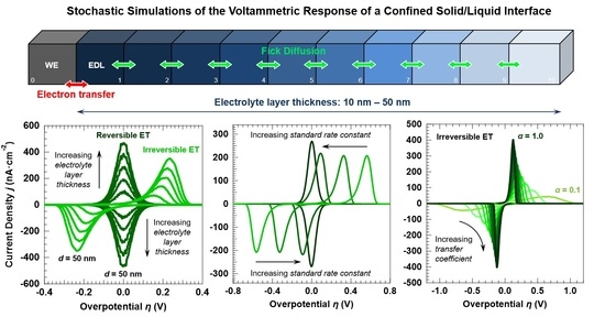
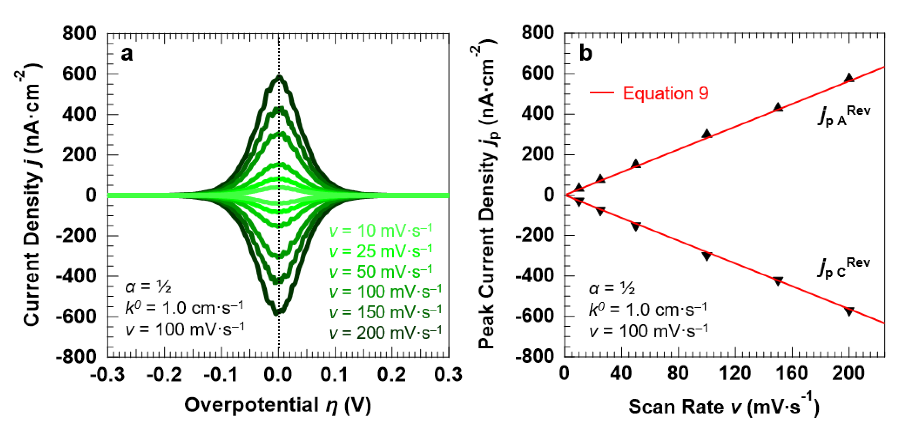
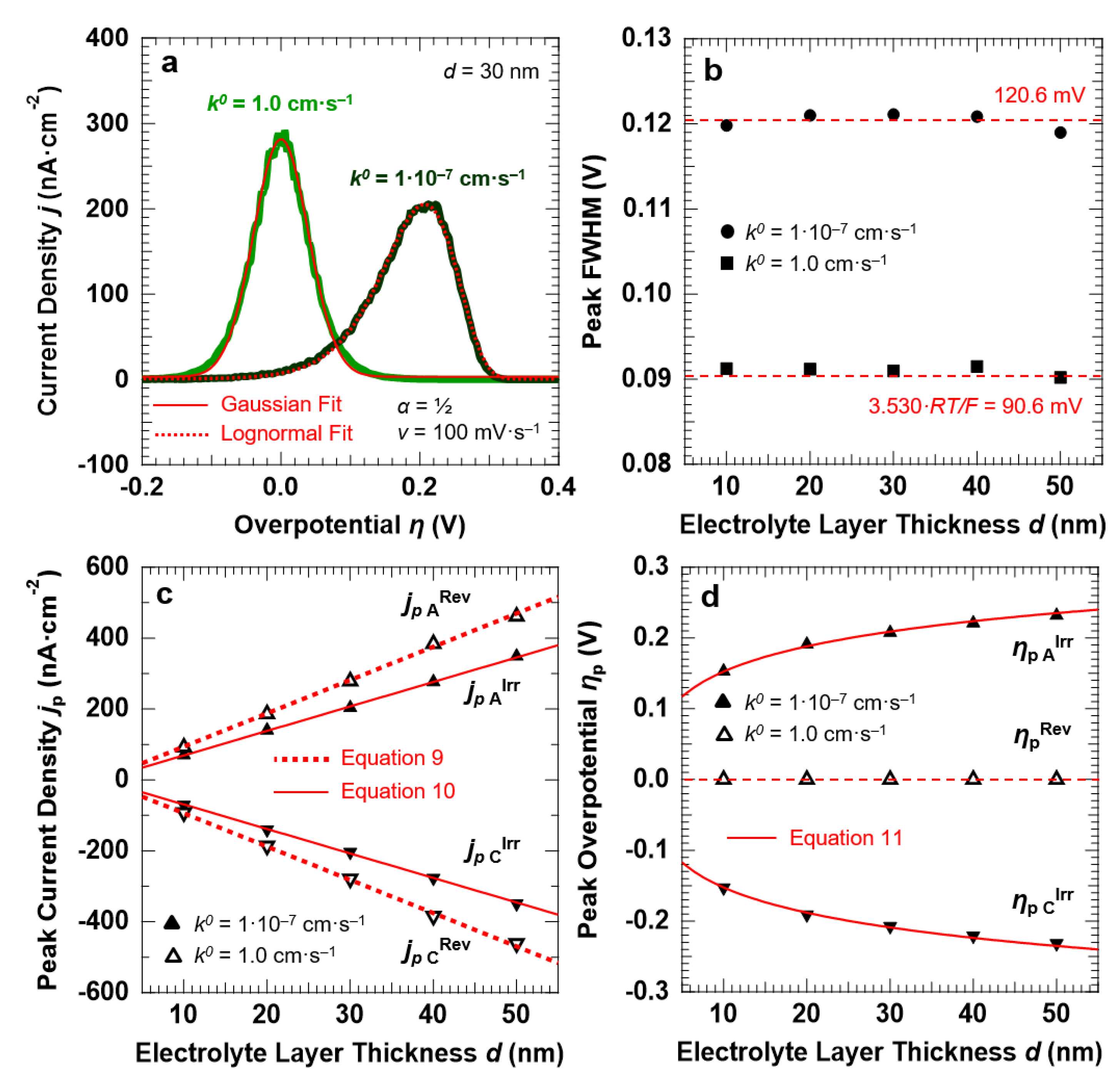
3.1. Voltammetric Response of the “Confined Interface” for a Symmetric (α = ½) ET as a Function of d (v = 100 mV·s1)

First, we focus our attention on the influence of the electrolyte layer thickness, d, on the voltammetric response of the “confined interface”. We carried out a series of simulations for two reaction kinetics, considering a reversible (fast) and an irreversible (sluggish) ET (k0 equal to 1.0 cm·s1 and 1.0 × 107 cm·s1, respectively). For both kinetics, we simulated a symmetric (α = ½) energy barrier. The CVs for the reversible and irreversible ET simulated at a scan rate of 100 mV·s1 are shown in Figure 3a,b, respectively, as a function of d (equal to 10, 20, 30, 40, and 50 nm).
For the reversible ET process (k0 = 1.0 cm·s−1), the anodic and cathodic peaks are symmetric around the standard potential of the redox couple (η = 0). This is confirmed by the fact that the peaks can be fitted with a single Gaussian function, as reported in Figure 4a for the anodic peak simulated for d = 30 nm and v = 100 mV·s−1. For the irreversible ET process (k0 = 1.0 × 10⁻⁷ cm·s−1), the voltammetric peaks are instead well-separated and exhibit a pronounced asymmetric tail at low overpotentials. The anodic peak reported in Figure 4a, obtained for the irreversible ET with d = 30 nm and v = 100 mV·s−1, shows that the line shape can be reproduced by using a Lognormal function. A decrease in the reaction rate not only induces an asymmetry of the peak line shape, but also causes a broadening of the voltammetric features (Figure 4b). A FWHM of 90.6 ± 1.4 mV is found for k0 = 1.0 cm·s−1, as expected for a Nernstian-reversible ET process at r.t [43]. For k0 = 1.0 × 10⁻⁷ cm·s−1, the peak FWHM for both the anodic and cathodic peaks is instead equal to 120.6 ± 1.2 mV.
Figure 4c shows the peak current density jp as a function of the electrolyte layer thickness, for the reversible and irreversible ET processes. The trend is linear in both cases, in agreement with the functional dependency outlined by Equations (10) and (11), respectively. Furthermore, the current density slightly decreases when passing from reversible to irreversible ET, with the corresponding ratio equal to 1.32. This is in agreement with the peak current density that results from the Hubbard’s model: Equations (9) and (10) provide, in fact, a ratio equal to 2.718/(4·α) = 1.36, for a symmetric energy barrier (α = ½).
Finally, the peak overpotential ηp (Figure 4d) is centered at η = 0 V for all the investigated d values for the reversible ET, whereas it shows a logarithmic dependency from d for k0 = 1.0 × 107 cm·s1, in agreement with Equation (11).

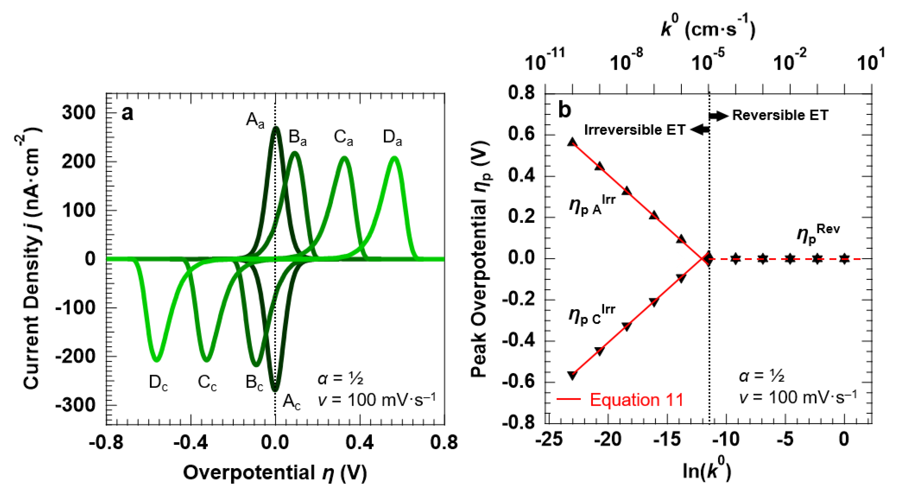
3.2. Voltammetric Response of the “Confined Interface” (d = 30 nm) for a Symmetric ET (α = ½) as a Function of k0

We simulated the electrochemical properties of the “confined interface” over a wide range of reaction kinetics, namely 10 orders of magnitude in k0, with a symmetric energy barrier (α = ½). Figure 5a reports the simulated CVs (at a fixed scan rate of 100 mV·s−1) for a reversible (A: k0 = 1.0 × 102 cm·s−1) and three irreversible ET processes (B: k0 = 1.0 × 106 cm·s−1, C: k0 = 1.0 × 108 cm·s−1, and D: k0 = 1.0 × 1010 cm·s−1).
Two observations can be made by comparing the reversible and the irreversible ET processes. First, the current density decreases when passing from reversible to irreversible ET, with the corresponding ratio equal to 1.32, as discussed above. For the irreversible ET process, we also observe that the peak current density remains constant for each simulated value of k0, in agreement with Equation (10). Second, strongly asymmetric anodic/cathodic peaks characterize the irreversible ET, as discussed above. The FWHM increases from 90.6 ± 1.3 mV (3.53·RT/F = 90.6 mV [43]) for the reversible ET to 120.6 ± 1.1 mV for all k0 < 1.0 × 105 cm·s−1. k0 = 1.0 × 105 cm·s−1 can therefore be taken as a value separating the reversible from the irreversible ET. This is confirmed by the negligible Δpp for k0 > 1.0 × 105 cm·s1, whereas for k0 < 1.0 × 105 cm·s1 the peak separation increases with decreasing reaction rates (Figure 5b). For values of k0 < 1.0 × 105 cm·s1, the trend of the overpotential ηp C,AIrr at which the voltammetric peaks are centered is linear with the natural logarithm of k0, in agreement with Hubbard’s model for an irreversible ET processes occurring in a confined environment (Equation (11)) [35].

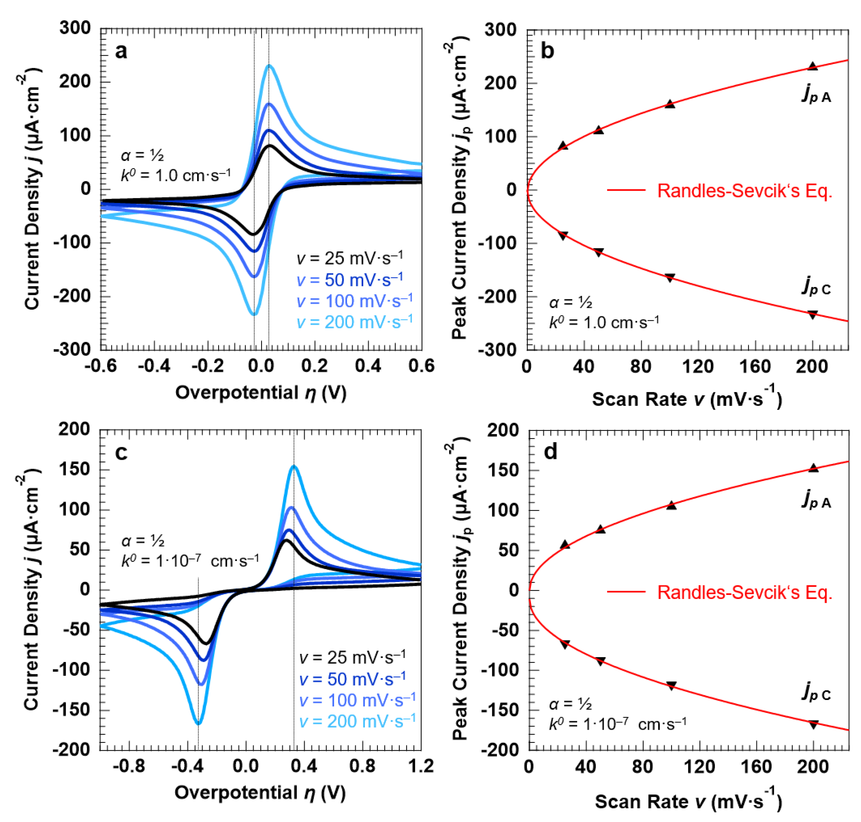
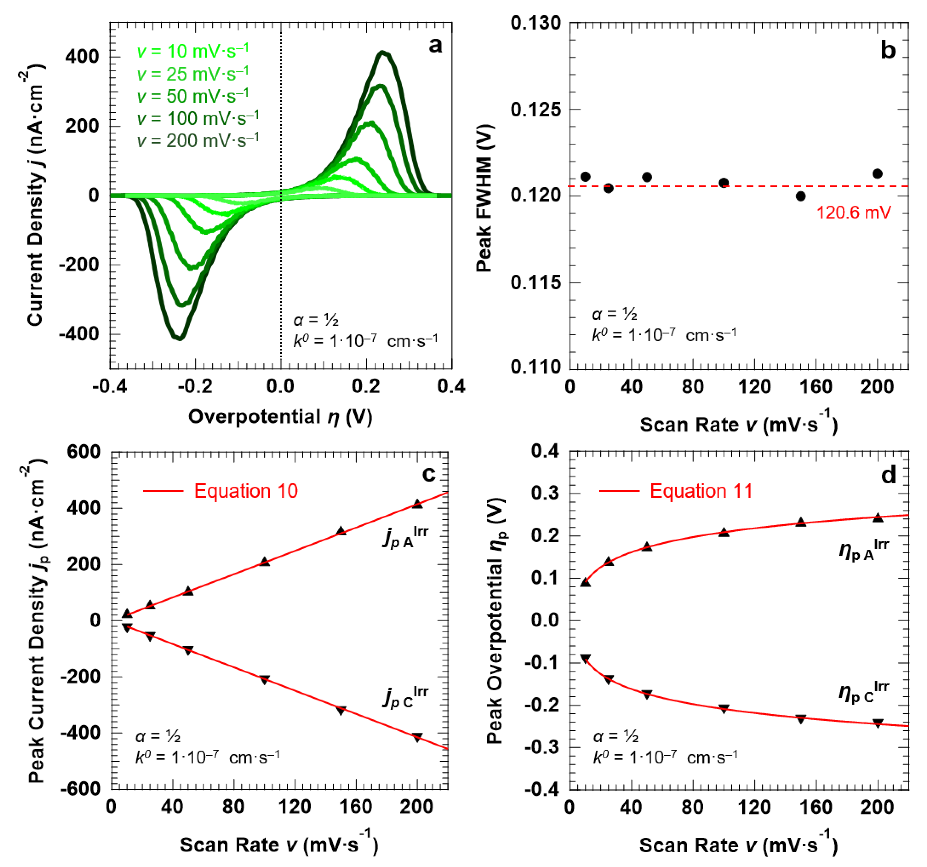
3.3. Voltammetric Response of the “Confined Interface” (d = 30 nm) for a Symmetric (α = ½) ET as a Function of v

We begin the analysis by simulating a (Nernstian-reversible) fast ET process between the redox couple in solution and the electrode surface, with α = 0.5 and k0 = 1.0 cm·s−1. To simulate the “confined interface”, the thickness of the electrolyte layer was set to 30.0 nm. The corresponding voltammetric response of the interface under the application of the overpotential with different scan rates is reported in Figure 6a. As expected for a reversible ET process, the line shape of the voltammetric peaks is purely Gaussian (with a FWHM of 90.6 ± 1.1 mV) and no separation exists between the anodic and cathodic peaks, which are centered at the equilibrium potential of the redox couple (η = 0 V, E = E°) irrespective of the scan rate. As Figure 6b shows, the current density at the anodic and cathodic peaks increases linearly with the potential scan rate, in line with the Hubbard’s model for a reversible ET (Equation (9)).
Let us now describe the “confined interface” for a symmetric (α = ½), irreversible ET (k0 = 1.0 × 107 cm·s1) as a function of the scan rate. The simulated CVs are reported in Figure 7a. The FWHM of both the anodic and cathodic peaks remains constant at around 120.6 ± 1.3 mV, thereby ruling out any effect of the scan rate on the broadening of the voltammetric waves. Finally, in agreement with Equations (10) and (11), the peak current density jp (Figure 7c) and overpotential ηp (Figure 7d) show a linear and logarithmic dependency on the scan rate, respectively.

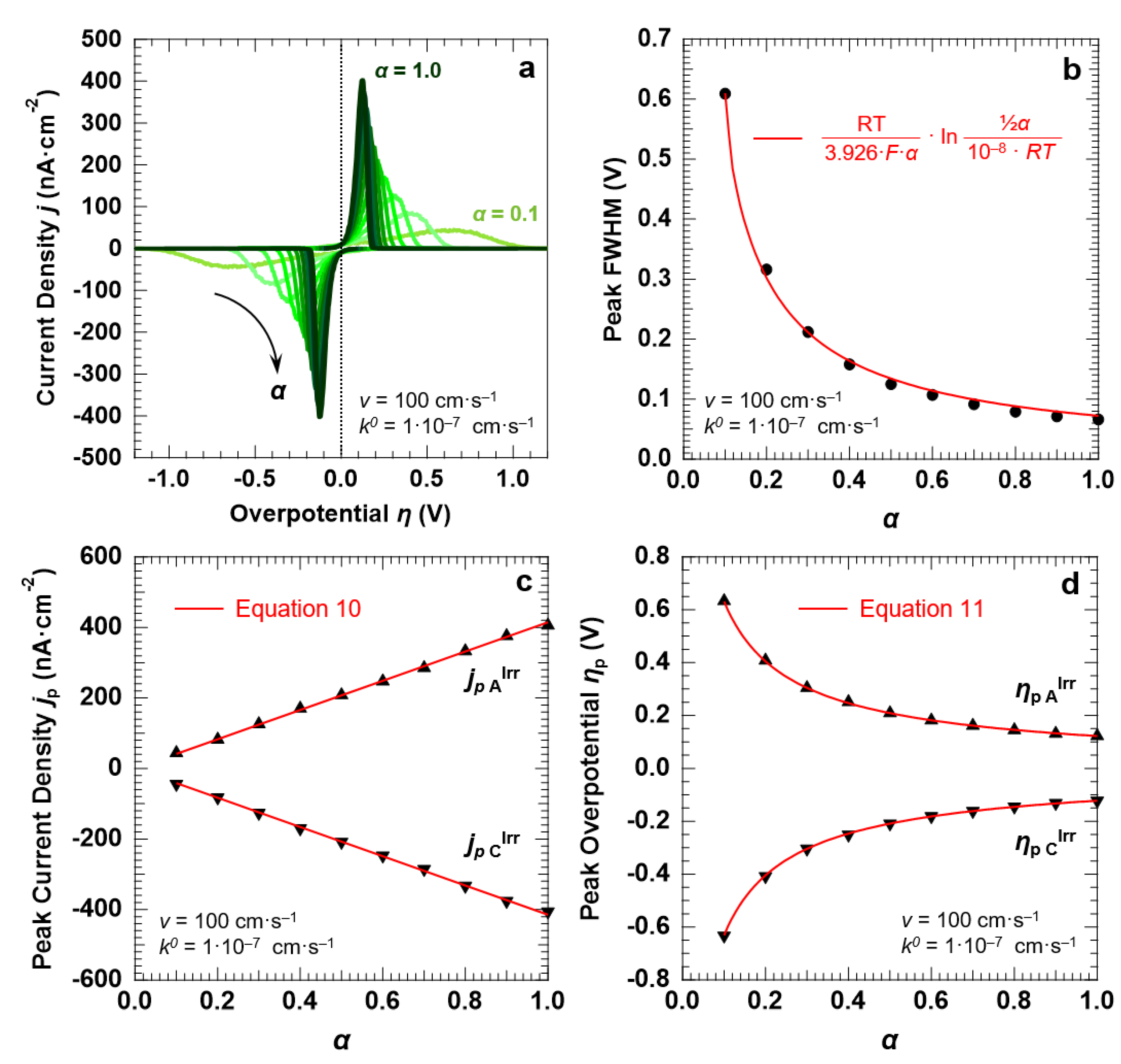
3.4. Voltammetric Response of the “Confined Interface” (d = 30 nm) for an Irreversible ET (k0 = 1.0 × 107 cm·s1) as a Function of α

Finally, to explore the influence of α on the voltammetric response of the “confined interface” (for d = 30 nm), we performed a series of simulations of an irreversible ET process (k0 = 1.0 × 107 cm·s1) with α spanning a range of 0.1–1.0 and a fixed potential scan rate of 100 mV·s1. The simulated CVs are reported in Figure 8a. It is clear that α has a strong influence on the FWHM, the magnitude, and the potential at which the voltammetric waves are centered. The FWHM of both the anodic and cathodic peaks decreases when α increases (Figure 8b). We found that the trend can be fitted with the following function (Equation (12)):
FWHMp A,C = RT/(3.926·F·α)·ln [½α/(10−8·RT)]
Note that for α = ½ Equation (12) provides a value of 120.6 mV, in agreement with the findings reported in the previous sections. With regard to the peak current density, Figure 8c shows that jp is directly proportional to α, in agreement with the predictions of the Hubbard’s model (Equation (10)). Similarly, the trend of the peak overpotential ηp as a function of α is well described by Equation (11), as shown by Figure 8d.

4. Conclusions

In conclusion, in this work we described the electrochemical properties of solid/liquid interfaces where the electrolyte layer thickness is limited to a few tens of nanometers. The investigation was performed using stochastic modeling of the electron transfer between a solid surface and a one-electron redox couple and its diffusion in solution. The following points summarize our findings and link them to existing experimental results obtained using in situ AP-XPS coupled with the “dip and pull” technique.
  • We show that the electrochemical response of nanometer-sized interfaces can be described with the thin-layer voltammetry theory originally elaborated by Hubbard for liquid layer thicknesses spanning from tens to hundreds of micrometers. For both space scales, the common dominant factor is that the diffusion of reactants is confined to the direction orthogonal to the interface. This is in agreement with our recent experimental work where the oxygen evolution reaction (OER) was investigated on a poly crystalline Pt surface immersed in 1.0M KOH aqueous solution [32]. Under those conditions, the hydroxyl anions present in the solution were depleted from the thin liquid layer due to the ongoing oxidation to molecular oxygen, eventually causing the loss of potential control at the interface [32]. We concluded that the applied overpotential (~700 mV with respect to the thermodynamic water oxidation potential, +1.23 V vs. RHE) sustained an electrolyte consumption rate in the thin electrolyte layer that was not counterbalanced on the same time scale by the diffusion rate from the macroscopic liquid meniscus.
  • We investigated the confined interface by simulating reversible and irreversible electron transfer processes as a function of the liquid layer thickness. For irreversible electron transfers, we find that the current density and the line shape of the voltammetric features are strongly dependent on the symmetry of the reactant and product free energy curves around the energy barrier. In addition, for both types of electron transfers, we observe that the current density is a linear function of the liquid layer thickness, and that the peak current density values are on the order of hundreds of nA·cm2 at most. It is noteworthy to compare this value with the one experimentally retrieved using two different working electrode configurations, as reported in ref. [13]: the first preserved the usual “dip and pull” geometry [7,13], while in the second one the bottom part of the sample immersed in the electrolyte was masked to approximate the current density reached at the “confined interface” [13]. We determined a current density ratio between the two experimental configurations of about 3, with the current density for the “masked” working electrode reaching some hundreds of μA·cm2 at most [13]. The discrepancy between this value and the one obtained in this work from the stochastic simulations can be easily explained in terms of the macroscopic liquid meniscus still present on the “masked” electrode, ensuring the necessary electrochemical continuity between the electrolyte layer on the sample and the bulk solution [13]. We use the capillary length as a “yardstick” to characterize the curvature of the meniscus, finding a value of about 4 mm for the liquid water/water vapor interface at r.t [47]. Therefore, although showing an expected decreasing trend when passing from a “bulk” to a “confined interface”, the current density values found in ref. [13] are dominated by the presence of the meniscus and do not capture the true properties of electrolyte layers with thicknesses limited to few tens of nanometers.
We believe that our results provide information about the fundamental electrochemical properties of electrolyte layers at the nanometer scale. Our approach and the corresponding results are general and valid for both aqueous and non-aqueous media. In particular, we believe that this study can contribute to a better understanding of the results obtained so far using the “dip and pull” method. In addition, we think that the findings described in this work can be beneficial for planning future experimental investigations using the same approach. For instance, the fact that the electrochemical current in such “confined interfaces” is ultimately limited by the reaction rate at the electrode opens up the possibility of directly investigating reaction kinetics coupling the “dip and pull” method with in situ time-resolved spectroscopies.

Funding

This research received no external funding.

Acknowledgments

The author thankfully acknowledges Francis A. Houle for the valuable discussions about Kinetiscope and its use to study chemical and electrochemical equilibria. Valuable discussions with David E. Starr, Roel van de Krol and Fatwa F. Abdi are also thankfully acknowledged.

Conflicts of Interest

The author declares no conflict of interest.

References

  1. Salmeron, M.; Schlögl, R. Ambient pressure photoelectron spectroscopy: A new tool for surface science and nanotechnology. Surf. Sci. Rep. 2008, 63, 169–199. [Google Scholar] [CrossRef] [Green Version]
  2. Crumlin, E.J.; Bluhm, H.; Liu, Z. In situ investigation of electrochemical devices using ambient pressure photoelectron spectroscopy. J. Electr. Spectr. Relat. Phenom. 2013, 190, 84–92. [Google Scholar] [CrossRef]
  3. Liu, X.; Yang, W.; Liu, Z. Recent progress on synchrotron-based in-situ soft X-ray spectroscopy for energy materials. Adv. Mater. 2014, 26, 7710–7729. [Google Scholar] [CrossRef] [PubMed]
  4. Crumlin, E.J.; Liu, Z.; Bluhm, H.; Yang, W.; Guo, J.; Hussain, Z. X-ray spectroscopy of energy materials under in situ/operando conditions. J. Elect. Spectr. Relat. Phenom. 2015, 200, 264–273. [Google Scholar] [CrossRef] [Green Version]
  5. Roy, K.; Artiglia, L.; van Bokhoven, J.A. Ambient Pressure Photoelectron Spectroscopy: Opportunities in Catalysis from Solids to Liquids and Introducing Time Resolution. Chem. Cat. Chem. 2018, 10, 666–682. [Google Scholar] [CrossRef]
  6. Lewerenz, H.-J.; Lichterman, M.F.; Richter, M.H.; Crumlin, E.J.; Hu, S.; Axnanda, S.; Favaro, M.; Drisdell, W.; Hussain, Z.; Brunschwig, B.S.; et al. Operando analyses of solar fuels light absorbers and catalysts. Electrochim. Acta 2016, 211, 711–719. [Google Scholar] [CrossRef] [Green Version]
  7. Favaro, M.; Abdi, F.F.; Crumlin, E.J.; Liu, Z.; van de Krol, R.; Starr, D.E. Interface science using ambient pressure hard X-ray photoelectron spectroscopy. Surfaces 2019, 2, 8. [Google Scholar] [CrossRef] [Green Version]
  8. Liu, Z.; Bluhm, H. Liquid/solid interfaces studied by ambient pressure HAXPES. In Hard X-ray Photoelectron Spectroscopy (HAXPES), 1st ed.; Woicik, J., Ed.; Springer: Cham, Switzerland, 2016; pp. 447–466. ISBN 978-3-319-24043-5. [Google Scholar]
  9. Axnanda, S.; Crumlin, E.J.; Mao, B.; Rani, S.; Chang, R.; Karlsson, P.G.; Edwards, M.O.M.; Lundqvist, M.; Moberg, R.; Ross, P.N.; et al. Using “tender” X-ray ambient pressure X-ray photoelectron spectroscopy as a direct probe of solid-liquid interface. Sci. Rep. 2015, 5, 9788. [Google Scholar] [CrossRef]
  10. Karslıoğlu, O.; Nemšák, S.; Zegkinoglou, I.; Shavorskiy, A.; Hartl, M.; Salmassi, F.; Gullikson, E.M.; Ng, M.L.; Rameshan, C.; Rude, B.; et al. Aqueous solution/metal interfaces investigated in operando by photoelectron spectroscopy. Faraday Discuss. 2015, 180, 35–53. [Google Scholar] [CrossRef] [Green Version]
  11. Favaro, M.; Jeong, B.; Ross, P.N.; Yano, J.; Hussain, Z.; Liu, Z.; Crumlin, E.J. Unravelling the electrochemical double layer by direct probing of the solid/liquid interface. Nat. Commun. 2016, 7, 12695. [Google Scholar] [CrossRef]
  12. Favaro, M.; Drisdell, W.S.; Marcus, M.A.; Gregoire, J.M.; Crumlin, E.J.; Haber, J.A.; Yano, J. An operando investigation of (Ni–Fe–Co–Ce)Ox system as highly efficient electrocatalyst for oxygen evolution reaction. ACS Catal. 2017, 7, 1248–1258. [Google Scholar] [CrossRef] [Green Version]
  13. Favaro, M.; Valero-Vidal, C.; Eichhorn, J.; Toma, F.M.; Ross, P.N.; Yano, J.; Liu, Z.; Crumlin, E.J. Elucidating the alkaline oxygen evolution reaction mechanism on platinum. J. Mater. Chem. A 2017, 5, 11634–11643. [Google Scholar] [CrossRef] [Green Version]
  14. Favaro, M.; Yang, J.; Nappini, S.; Magnano, E.; Toma, F.M.; Crumlin, E.J.; Yano, J.; Sharp, I.D. Understanding the oxygen evolution reaction mechanism on CoOx using operando ambient-pressure X-ray photoelectron spectroscopy. J. Am. Chem. Soc. 2017, 139, 8960–8970. [Google Scholar] [CrossRef] [PubMed] [Green Version]
  15. Shavorskiy, A.; Ye, X.; Karslıoğlu, O.; Poletayev, A.D.; Hartl, M.; Zegkinoglou, I.; Trotochaud, L.; Nemšák, S.; Schneider, C.M.; Crumlin, E.J.; et al. Direct mapping of band positions in doped and undoped hematite during photoelectrochemical water splitting. J. Phys. Chem. Lett. 2017, 8, 5579–5586. [Google Scholar] [CrossRef] [Green Version]
  16. Calvillo, L.; Fittipaldi, D.; Rüdiger, C.; Agnoli, S.; Favaro, M.; Valero-Vidal, C.; Di Valentin, C.; Vittadini, A.; Bozzolo, N.; Jacomet, S.; et al. Carbothermal Transformation of TiO2 into TiOxCy in UHV: Tracking Intrinsic Chemical Stabilities. J. Phys. Chem. C 2014, 118, 22601–22610. [Google Scholar] [CrossRef]
  17. Stoerzinger, K.A.; Favaro, M.; Ross, P.N.; Yano, J.; Liu, Z.; Hussain, Z.; Crumlin, E.J. Probing the Surface of Platinum during the Hydrogen Evolution Reaction in Alkaline Electrolyte. J. Phys. Chem. B 2018, 122, 864–870. [Google Scholar] [CrossRef] [Green Version]
  18. Gokturk, P.A.; Camci, M.T.; Suzer, S. Lab-based operando x-ray photoelectron spectroscopy for probing low-volatile liquids and their interfaces across a variety of electrosystems. J. Vac. Sci. Technol. A 2020, 38, 040805. [Google Scholar] [CrossRef]
  19. Novotny, Z.; Aegerter, D.; Comini, N.; Tobler, B.; Artiglia, L.; Maier, U.; Moehl, T.; Fabbri, E.; Huthwelker, T.; Schmidt, T.J.; et al. Probing the solid–liquid interface with tender x rays: A new ambient-pressure x-ray photoelectron spectroscopy endstation at the Swiss Light Source. Rev. Sci. Instrum. 2020, 91, 023103. [Google Scholar] [CrossRef]
  20. Starr, D.E.; Favaro, M.; Abdi, F.F.; Bluhm, D.; Crumlin, E.J.; van de Krol, R. Combined soft and hard X-ray ambient pressure photoelectron spectroscopy studies of semiconductor/electrolyte interfaces. J. Elect. Spectr. Relat. Phenom. 2017, 221, 106–115. [Google Scholar] [CrossRef] [Green Version]
  21. Velasco-Vélez, J.J.; Pfeifer, V.; Hävecker, M.; Wang, R.; Centeno, A.; Zurutuza, A.; Algara-Siller, G.; Stotz, E.; Skorupska, K.; Teschner, D.; et al. Atmospheric pressure X-ray photoelectron spectroscopy apparatus: Bridging the pressure gap. Rev. Sci. Instrum. 2016, 87, 053121. [Google Scholar] [CrossRef]
  22. Velasco-Vélez, J.J.; Pfeifer, V.; Hävecker, M.; Weatherup, R.S.; Arrigo, R.; Chuang, C.-H.; Stotz, E.; Weinberg, G.; Salmeron, M.; Schlögl, R.; et al. Photoelectron spectroscopy at the graphene-liquid interface reveals the electronic structure of an electrodeposited cobalt/graphene electrocatalyst. Angew. Chem. Int. Ed. 2015, 54, 14554–14558. [Google Scholar] [CrossRef] [PubMed] [Green Version]
  23. Rik, M.; Frevel, L.; Velasco-Vélez, J.J.; Plodinec, M.; Knop-Gericke, A.; Schlögl, R. The Oxidation of Platinum under Wet Conditions Observed by Electrochemical X-ray Photoelectron Spectroscopy. J. Am. Chem. Soc. 2019, 141, 6537–6544. [Google Scholar] [CrossRef] [PubMed]
  24. Velasco-Velez, J.-J.; Mom, R.V.; Sandoval-Diaz, L.-E.; Falling, L.J.; Chuang, C.-H.; Gao, D.; Jones, T.E.; Zhu, Q.; Arrigo, R.; Roldan Cuenya, B.; et al. Revealing the Active Phase of Copper during the Electroreduction of CO2 in Aqueous Electrolyte by Correlating In Situ X-ray Spectroscopy and In Situ Electron Microscopy. ACS Energy Lett. 2020, 5, 2106–2111. [Google Scholar] [CrossRef] [PubMed]
  25. Lichterman, M.F.; Hu, S.; Richter, M.H.; Crumlin, E.J.; Axnanda, S.; Favaro, M.; Drisdell, W.; Hussain, Z.; Mayer, T.; Brunschwig, B.S.; et al. Direct observation of the energetics at a semiconductor/liquid junction by operando X-ray photoelectron spectroscopy. Energy Environ. Sci. 2015, 8, 2409–2416. [Google Scholar] [CrossRef] [Green Version]
  26. Kolb, D.M.; Hansen, W.N. Electroreflectance spectra of emersed metal electrodes. Surf. Sci. 1979, 79, 205–211. [Google Scholar] [CrossRef]
  27. Hansen, W.N. Electrode resistance and the emersed double layer. Surf. Sci. 1980, 101, 109–122. [Google Scholar] [CrossRef]
  28. Kolb, D.M.; Rath, D.L.; Wille, R.; Hansen, W.N. An ESCA study on the electrochemical double layer of emersed electrodes. Ber. Bunsenges. Phys. Chem. 1983, 87, 1108. [Google Scholar] [CrossRef]
  29. Siegbahn, H. Electron spectroscopy for chemical analysis of liquids and solutions. J. Phys. Chem. 1985, 89, 897–909. [Google Scholar] [CrossRef]
  30. Weingarth, D.; Foelske-Schmitz, A.; Wokaun, A.; Kötz, R. In situ electrochemical XPS study of the Pt/[EMIM][BF4] system. Electrochem. Comm. 2011, 13, 619–622. [Google Scholar] [CrossRef]
  31. Booth, S.G.; Tripathi, A.M.; Strashnov, I.; Dryfe, R.A.W.; Walton, A.S. The offset droplet: A new methodology for studying the solid/water interface using X-ray photoelectron spectroscopy. J. Phys. Condens. Matter 2017, 29, 454001. [Google Scholar] [CrossRef] [Green Version]
  32. Stoerzinger, K.A.; Favaro, M.; Ross, P.N.; Hussain, Z.; Liu, Z.; Yano, J.; Crumlin, E.J. Stabilizing the meniscus for operando characterization of platinum during the electrolyte-consuming alkaline oxygen evolution reaction. Top. Catal. 2018, 61, 2152–2160. [Google Scholar] [CrossRef] [Green Version]
  33. Favaro, M.; Abdi, F.F.; Lamers, M.; Crumlin, E.J.; Liu, Z.; van de Krol, R.; Starr, D.E. Light-induced surface reactions at the bismuth vanadate/potassium phosphate interface. J. Phys. Chem. B 2018, 122, 801–809. [Google Scholar] [CrossRef] [PubMed]
  34. Kinetiscope Web Site. Available online: http://hinsberg.net/kinetiscope/index.html (accessed on 7 August 2020).
  35. Hubbard, A.T. Study of the kinetics of electrochemical reactions by thin-layer voltammetry: I. Theory. J. Electroanal. Chem. 1969, 22, 165–174. [Google Scholar] [CrossRef]
  36. Houle, F.A.; Hinsberg, W.D.; Morrison, M.; Sanchez, M.I.; Wallraff, G.; Larson, C.; Hoffnagle, J. Determination of coupled acid catalysis-diffusion processes in a positive-tone chemically amplified photoresist. J. Vac. Sci. Technol. B Microelectron. Nanometer Struct. Process. Meas. Phenom. 2000, 18, 1874. [Google Scholar] [CrossRef]
  37. Houle, F.A.; Hinsberg, W.D.; Sanchez, M.I. Kinetic Model for Positive Tone Resist Dissolution and Roughening. Macromolecules 2002, 35, 8591–8600. [Google Scholar] [CrossRef]
  38. Bard, A.J.; Faulkner, L.R. Electrochemical Methods, 2nd ed.; John Wiley & Sons Inc.: Hoboken, NJ, USA, 2001; Appendix B; ISBN 13 978-0-471-04372-0. [Google Scholar]
  39. Wiegel, A.A.; Wilson, K.R.; Hinsberg, W.D.; Houle, F.A. Stochastic methods for aerosol chemistry: A compact molecular description of functionalization and fragmentation in the heterogeneous oxidation of squalane aerosol by OH radicals. Phys. Chem. Chem. Phys. 2015, 17, 4398–4411. [Google Scholar] [CrossRef] [PubMed] [Green Version]
  40. Lee, L.L. Molecular Thermodynamics of Electrolyte Solutions; World Scientific Publishing Co. Pte. Ltd.: Singapore, 2008; Chapter 11; ISBN 13 978-981-281-418-0. [Google Scholar]
  41. Archer, G.G.; Wang, P. The Dielectric Constant of Water and Debye-Hückel Limiting Law Slopes. J. Phys. Chem. Ref. Data 1990, 19, 371–411. [Google Scholar] [CrossRef] [Green Version]
  42. Bauer, H.H. The electrochemical transfer-coefficient. J. Electroanal. Chem. Interf. Electrochem. 1968, 16, 419–432. [Google Scholar] [CrossRef]
  43. Salbeck, J. An electrochemical cell for simultaneous electrochemical and spectroelectrochemical measurements under semi-infinite diffusion conditions and thin-layer conditions. J. Electroanal. Chem. 1992, 340, 169–195. [Google Scholar] [CrossRef]
  44. Favaro, M.; Perini, L.; Agnoli, S.; Durante, C.; Granozzi, G.; Gennaro, G. Electrochemical behavior of N and Ar implanted highly oriented pyrolytic graphite substrates and activity toward oxygen reduction reaction. Electrochim. Acta 2013, 88, 477–487. [Google Scholar] [CrossRef]
  45. Favaro, M.; Agnoli, S.; Cattelan, M.; Moretto, A.; Durante, C.; Leonardi, S.; Kunze-Liebhäuser, J.; Schneider, O.; Gennaro, A.; Granozzi, G. Shaping graphene oxide by electrochemistry: From foams to self-assembled molecular materials. Carbon 2014, 77, 405–415. [Google Scholar] [CrossRef]
  46. Botasini, S.; Mendez, E. Limited Diffusion and Cell Dimensions in a Micrometer Layer of Solution: An Electrochemical Impedance Spectroscopy Study. Chem. Electro. Chem. 2017, 4, 1891–1895. [Google Scholar] [CrossRef]
  47. Boucher, E.A. Capillary phenomena: Properties of systems with fluid/fluid interfaces. Rep. Prog. Phys. 1980, 43, 497–546. [Google Scholar] [CrossRef]
Figure 1. Solid/liquid interface parametrization used in this work. The elements from 1 to 10 represent the electrolyte solution atop the WE surface (element 0), with element 1 simulating the EDL. The colored arrows indicate electron transfer (ET) and Fick diffusion (FD) between the different elements. The right inset reports the schematization of the two possible diffusion pathways (DP), parallel and orthogonal to the interface.
Surfaces 03 00029 g001
Figure 2. Simulation results of a symmetric (α = 0.5), Nernstian-reversible (k0 = 1.0 cm·s−1 (a,b) and irreversible ET (k0 = 1.0 × 10⁻⁷ cm·s−1 (c,d) for a “bulk interface” (d = 1320 µm). For both set of simulations, the initial concentration of the oxidized and reduced species in solution was set to 0.5 mM, for a total concentration of the redox couple equal to 1.0 mM. (a,c) and (b,d) report the simulated cyclic voltammograms and the corresponding peak current densities as a function of the potential scan rate v. For both ET processes, the simulations show that the peak current density obeys the Randles–Sevcik equation.
Surfaces 03 00029 g002
Figure 3. Simulation results for a symmetric (α = ½) ET between the redox couple in solution and the electrode surface, as a function of d (at a fixed scan rate v of 100 mV·s−1); (a) reversible ET (k0 = 1.0 cm·s−1); (b) irreversible ET (k0 = 1.0 × 10⁻⁷ cm·s−1). For both sets of simulations, the initial concentration of the oxidized and reduced species in solution was set to 0.5 mM, for a total concentration of the redox couple equal to 1.0 mM.
Surfaces 03 00029 g003
Figure 4. (a): Anodic peaks and corresponding Gaussian and Lognormal fits for a reversible (k0 = 1.0 cm·s−1) and irreversible ET (k0 = 1.0 × 10⁻⁷ cm·s−1), respectively. The simulations were carried out for a symmetric energy barrier (α = ½) and setting d = 30 nm and v = 100 mV·s−1. Trends of the peak FWHM (b), current density jp (c), and overpotential ηp (d) as a function of the electrolyte layer thickness d (symbols). The figures also report the corresponding predictions of the Hubbard’s model (red lines).
Surfaces 03 00029 g004
Figure 5. Simulation results for a symmetric ET (α = ½) between the redox couple in solution and the electrode surface, with d = 30.0 nm. (a) CVs simulated at a scan rate v of 100 mV·s−1, as a function of the standard rate constant k0 (A: k0 = 1.0 × 10⁻² cm·s−1, B: k0 = 1.0 × 10⁻⁶ cm·s−1, C: k0 = 1.0 × 10⁻⁸ cm·s−1, D: k0 = 1.0 × 10⁻¹⁰ cm·s−1). (b) Overpotentials ηp A and ηp C at which the anodic and cathodic waves are centered as a function of k0 and its natural logarithm (full symbols). The solid red lines describe the ηp AIrr and ηp CIrr trends as predicted by the Hubbard’s model (Equation (11)), whereas ηp Rev = 0 V (E = E°) for a Nernstian-reversible ET (k0 > 1.0 × 10⁻⁵ cm·s−1). The initial concentration of the oxidized and reduced species in solution was set to 0.5 mM, for a total concentration of the redox couple equal to 1.0 mM.
Surfaces 03 00029 g005
Figure 6. Simulation results of a symmetric (α = 0.5), Nernstian-reversible ET (k0 = 1.0 cm·s−1) between the redox couple in solution and the electrode surface, for a “confined interface” (d = 30 nm). (a,b) Simulated voltammetric response and corresponding peak current densities as a function of the potential scan rate v. The initial concentration of the oxidized and reduced species in solution was set to 0.5 mM, for a total concentration of the redox couple equal to 1.0 mM.
Surfaces 03 00029 g006
Figure 7. Simulation results for a symmetric (α = ½), irreversible ET (k0 = 1.0 × 10⁻⁷ cm·s−1) between the redox couple in solution and the electrode surface, with d = 30.0 nm. (a) Simulated CVs as a function of the scan rate v. The trends of the peak FWHM, current density jp, and overpotential ηp as a function of v (full symbols) are reported in (bd), respectively, together with the corresponding predictions of the Hubbard’s model (solid red lines). The initial concentration of the oxidized and reduced species in solution was set to 0.5 mM, for a total concentration of the redox couple equal to 1.0 mM.
Surfaces 03 00029 g007
Figure 8. Simulation results for an irreversible ET (k0 = 1.0 × 10⁻⁷ cm·s−1) between the redox couple in solution and the electrode surface, with d = 30 nm. (a) CVs simulated at a scan rate v of 100 mV·s−1, as a function of the transfer coefficient α. The trends of the peak FWHM, current density jp, and overpotential ηp as a function of α (full symbols) are reported in (bd), respectively, together with the corresponding predictions of the Hubbard’s model (solid red lines). The initial concentration of the oxidized and reduced species in solution was set to 0.5 mM, for a total concentration of the redox couple equal to 1.0 mM.
Surfaces 03 00029 g008
Table 1. Diffusion layer thickness l for all the investigated potential sweep ranges and scan rates. The values of l have been determined using Equation (3) and the diffusion coefficient D of the redox couple, equal to 0.5 × 10⁻⁵ cm2·s−1. The electrochemical “bulk” conditions are guaranteed by the total thickness of the liquid layer atop the electrode surface (d = 1320 µm), which exceeds l for all the investigated parameters.
Potential Scan Rate v (mV·s−1)Potential Sweep Duration Δt (s) for ΔV = 1.2 VDiffusion Layer Thickness l (µm) for ΔV = 1.2 V
2548930
5024660
10012465
2006330
Table 2. Δx dimensions for the liquid elements used to simulate a total electrolyte layer thickness of 10, 20, 30, 40, and 50 nm.
Liquid Electrolyte Layer Thickness d (nm)Δx Element 1 (EDL) (nm) 1Δx Elements 2–10 (nm)
102.880.79
202.881.90
302.883.01
402.884.12
502.885.24
1 EDL thickness (defined as 3·k−1) for a supporting electrolyte concentration of 0.1 M (see text for details).

