Machine Learning Forecasting of Direct Solar Radiation: A Multi-Model Evaluation with Trigonometric Cyclical Encoding

Abstract

As the world is shifting toward cleaner energy sources, accurate forecasting of solar radiation is critical for optimizing the performance and integration of solar energy systems. In this study, we explore eight machine learning models, namely, Random Forest Regressor, Linear Regression Model, Artificial Neural Network, k-Nearest Neighbors, Support Vector Regression, Gradient Boosting Regressor, Gaussian Process Regression, and Deep Learning, as to their use in forecasting direct solar radiation across six climatically diverse regions in the Kingdom of Saudi Arabia. The models were evaluated using eight statistical metrics along with time-series and absolute error analyses. A key contribution of this work is the introduction of Trigonometric Cyclical Encoding, which has significantly improved temporal representation learning. Comparative SHAP-based feature-importance analysis revealed that Trigonometric Cyclical Encoding enhanced the explanatory power of temporal features by 49.26% for monthly cycles and 53.30% for daily cycles. The findings show that Deep Learning achieved the lowest root mean square error, as well as the highest coefficient of determination, while Artificial Neural Network demonstrated consistently high accuracy across the sites. Support Vector Regression performed optimally but was less reliable in some regions. Error and time-series analyses reveal that Artificial Neural Network and Deep Learning maintained stable prediction accuracy throughout high solar radiation seasons, whereas Linear Regression, Random Forest Regressor, and k-Nearest Neighbors showed greater fluctuations. The proposed Trigonometric Cyclical Encoding technique further enhanced model performance by maintaining the overall fitness of the models, which ranged between 81.79% and 94.36% in all scenarios. This paper supports the effective planning of solar energy and integration in challenging climatic conditions.

1. Introduction

Concerns about climate change and the exhaustion of conventional fuels have forced the world to move at a fast pace, over the last few decades, towards a global transition in energy production, changing from traditional fossil fuel-based sources to environmentally friendly sources [1,2,3]. Among the technologically mature and commercially acceptable sources, solar energy has risen to prominence in recent times as a clean source of energy, because it places less stress on the natural environment and can be integrated into urban areas, providing greater environmental comfort [4,5]. According to IRENA, renewable energy alone accounted for 86% of global power additions in 2023, largely due to enormous growth in solar and wind power [6,7]. This growth is mostly associated with improvements of technology and decreases in cost, as well as the proper government and institutional policies and frameworks that have made the utilization of solar energy more feasible and affordable [8,9].

However, solar power generation is variable and depends largely on weather, climate, and temporal patterns. The unpredictability of solar electricity generation is a significant barrier to blending solar power into the already existing power infrastructure. As discussed in [10], the fluctuating behaviour of solar resources is influenced by meteorological conditions, thereby creating uncertainty in estimating the power generation. A study by [11] has shown that enhanced forecasting can improve the efficiency of the plant operations by up to 15% and the integration costs can also be cut down to a large extent. Solar forecasting could be applied to tasks including scheduling the use and storage of solar energy, evaluating and forecasting the performance of existing solar installations, sizing solar installations, ensuring timely scheduled maintenance, and assessing the capacity and demands of electricity networks [12].

Two main techniques, the empirical and ML models, are prominently discussed in the literature as efficient ways of estimating and forecasting the incoming solar energy by learning from a historical time series associated with a particular geographical setting [13]. The study described in [14] reported a new technique, integrating several ML models with RFE, and obtained a great success compared with the performance of the LR model (RMSE = 0.003, R² = 0.999). Also, ref. [15] has shown that combining multiple ML algorithms and utilizing ensemble voting with weighted averaging gives commendable results: a 6% decrease in MAE, 3% in RMSE, and 16% in MAPE [16,17].

When building an ML model for a particular geographic location, certain features contribute to its architecture. The authors of [18,19] reported SVR-BO as being the optimal performer for Moroccan climatic conditions (RMSE = 0.4473). On the other hand, ref. [20] found that the best-performing algorithms differ from site to site. There are also more advanced strategies that combine multiple methods, and which are starting to yield better progress-for instance, ref. [21] combined LibRadtran RTM and ML models and achieved an R² value of 0.98, but their work was limited to clear sky conditions. Likewise, ref. [22] proposed an ADSSOA-LSTM which led to a low RMSE of 0.000388, increasing, however, the computational burden.

The KSA stands out as one of the world’s top locations for capturing solar energy. Forecasting solar radiation accurately is an important step in the planning, design, and utilization of solar energy systems [23]. The present study focuses on the performance evaluation of eight ML algorithms for six distinct sites in the KSA, representing a geographical distribution within the coastal, inland, northern, and western flanks of the kingdom, each area of which features different altitudes and topography. Meteorological data were sourced from NASA POWER on daily basis, within a period spanning 1 January 2023 to 31 December 2023, for all sites. ML algorithms were evaluated using a wide range of metrics (MBE, RMSE, rRMSE, MABE, MAPE, R², t-stat, MSE, and MAE) to offer a reliable assessment of the prediction accuracy [24]. In this paper, the terms “direct solar radiation” and “beam solar radiation” are used interchangeably, as both refer to the Direct Normal Irradiance (DNI) component of solar energy. The present study seeks to address the gap in location-specific insights into ML model efficacy, contributing to the identification and selection of optimal algorithms for accurate solar energy forecasting within varied geographical contexts across the region of the Middle East, and particularly for the case of the KSA [25].

Table 1. Summary of the literature review.

Ref.	Methodology	Key Findings	Limitations
[26]	Predicts daily global solar radiation data for 6 Pakistani cities	SVR achieves the best performance, with R2 values up to 0.99	No FE; No feature selection reported
[27]	Ensemble ML algorithms for solar power prediction in Saudi Arabia	RF outperformed other models (MAE = 0.0141), (RMSE = 0.0211)	Limited to Dhahran Limited evaluation metrics
[28]	Multiple ML models (RF, GBM, LR, CART, and DT)	LR and RF achieved lowest nMAE (−0.144, −0.151)	Limited feature-selection methods
[29]	Compares RF with hyperparameter optimization to other ML models	95.98% accuracy with optimized RF	Limited to Queretaro, Mexico; Focused on short-term predictions
[30]	Comparative analysis of BiLSTM-based LSTNet	RF-LSTNet performed best	Limited explanation of feature-selection process
[15]	Multiple ML algorithms (RF, XGBoost, and CatBoost)	Best performance with RF and CatBoost combination	Limited to Brazilian region
[31]	WRF Solar model	Superior performance compared to baseline models	Region-specific (Northwest China)
[21]	Comparison of six ML approaches	RTM-RF showed best performance (MAE 15.57 W/m2)	Limited to clear sky conditions
[19]	Comparison of 5 ML models with/without BO	SVR-BO performed best (RMSE = 0.4473 kWh/m2/day)	Single location study (Fez, Morocco); Limited feature set
[32]	Radial Basis Function Neural Network (RBF-NN) for DSR and DNR	DSR; MAPE = 1.6–9.3% DNR; MAPE= 0.49–41%	Relatively old dataset (1998–2002)
[33]	Review of ML techniques	Decision trees, RF, XGBoost, and SVM are effective ML models	Inadequate use of FE; Limited context for the KSA
[20]	Multiple metaheuristic algorithms (GBO, HHO, BMO, SCA, and HGSO) for distinct locations in Turkey	SCA best for Afyonkarahisar; GBO best for Ağrı	Limited input variables
[22]	ADSSOA-LSTM hybrid comparison with GA, PSO, and GWO	ADSSOA-LSTM achieved lowest RMSE (0.000388)	Limited feature exploration
[34]	Comparison of multiple ML algorithms	XGBoost showed highest performance	Single-location study
[35]	Comparison of next-gen ML algorithms	Random Forest outperformed other algorithms; MLP-ANN improved with feature selection	Limited to single application

summarises the research findings of the most recent works in the literature, along with the relevant methodologies and the limitations relevant to these studies.

2. Methodology

This paper adopts a structured ML pipeline to evaluate the performance of eight algorithms in forecasting DNI across six climatically diverse sites in the KSA. The methodology includes site selection and data acquisition, data preprocessing, exploratory data analysis, and temporal feature engineering using Trigonometric Cyclic Encoding (TCE), followed by model training and an exhaustive hyperparameter optimization tailored for each site and ML algorithm. A comprehensive set of statistical metrics is then used to assess model accuracy. Figure 1 presents a step-by-step flowchart of the methodological approach undertaken in the present study.

2.1. Case-Study Area Examination

The KSA has been touted as a hotspot for harnessing solar energy, due to its unique geographic positioning, which allows it to enjoy high levels of solar irradiance [27,36]. The present study focuses on six key strategic sites representing diverse climatic and geographical regions in the KSA. These sites were carefully selected to ensure a wide coverage of different altitudes, terrains, and solar radiation profiles, to provide a robust foundation for evaluating and assessing the performance of the ML algorithms.

Table 2. Geographical overview of case-study areas.

Location	Region	Latitude (°N)	Longitude (°E)	Altitude (m)
Tabuk	Northern	28.3835	36.5662	695
Riyadh	Central	24.7136	46.6753	630
Dhahran	Eastern	26.2869	50.1140	10
Najran	Southern	17.5656	44.2289	1742
Jeddah	Western	21.4858	39.1925	12
Al-Jouf	Northern	29.8679	40.1000	680

presents key geographic information about the six case-study sites considered in this study.

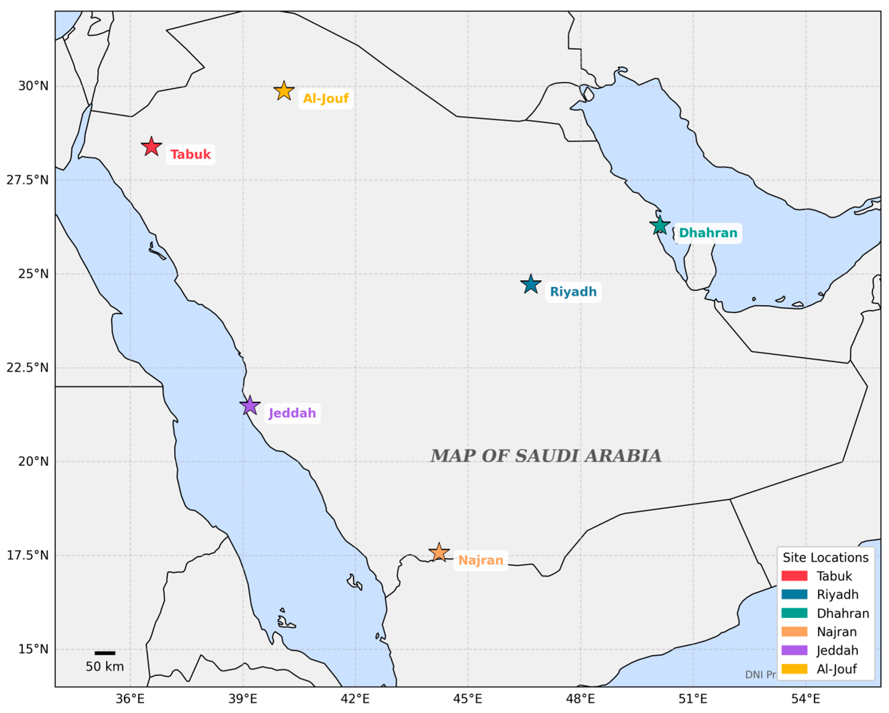
Figure 2 presents the geographic distribution and locations of the six selected case-study sites-Riyadh, Dhahran, Jeddah, Najran, Tabuk, and Al-Jouf—spread across diverse climatic zones in the KSA.

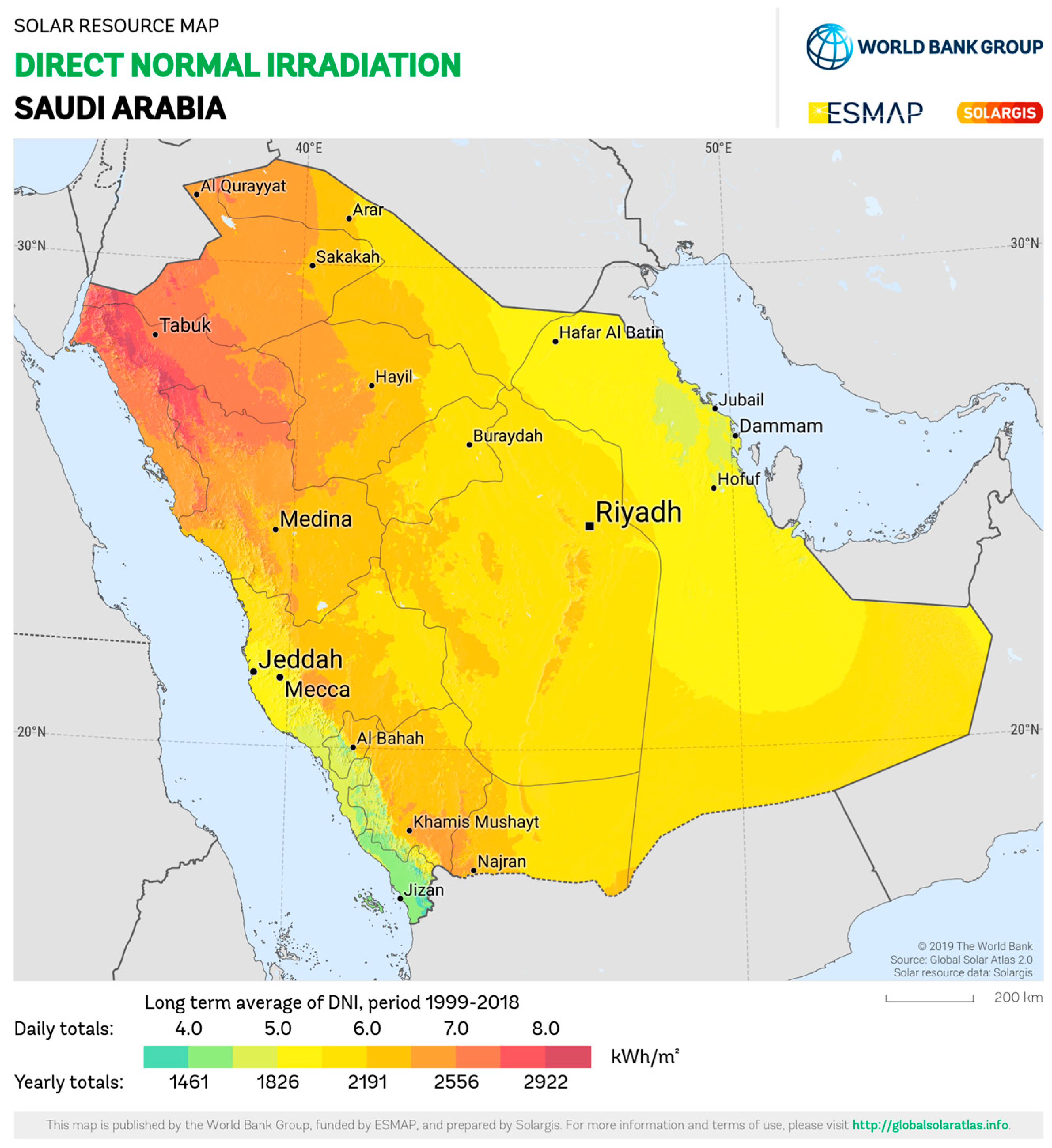
Figure 3 offers a comprehensive overview of DNI resource outlook across the KSA. Figure 3 showcases the extended term averages of both yearly and daily DNI accumulations specific to the KSA.

2.2. Meteorological Data Overview

The data used was sourced from the NASA POWER database. In the present study, essential variables (input features), including date, temperature, relative humidity, all-sky clearness index, and wind speed, were sourced on a daily basis from 1 January 2023, to 31 December 2023, aligning with methodologies outlined in previous studies examining solar energy feasibility in the Kingdom of Saudi Arabia and elsewhere [37,38]. This dataset encompasses 365 row entries of daily datapoints, with 8 columns representing 7 input features and 1 target variable for all six sites. The target variable, labelled “All-Sky Surface Shortwave Downward Direct Normal Irradiance”, explicitly represents the direct component of solar radiation incident on a surface normal to the sun’s rays under all-sky conditions (i.e., including the effects of clouds). The metadata and a description of the meteorological data collected are presented in

Table 3. Description of the meteorological data [39].

Feature	Description	Unit
DT	Date	-
MO	Month	-
DY	Day	-
HR	Hour	hr
TMP	Temperature at 2 m	°C
RH	Relative Humidity at 2 m	%
CI	All-Sky Insolation Clearness Index	dimensionless
WS	Wind Speed at 10 m	m/s
DNI	All-Sky Surface Shortwave Downward Irradiance	kWh/m2/day

.

2.3. ML Algorithms

Eight ML algorithms were selected for evaluation in this study due to their known utility in non-linear regression and solar-forecasting tasks [40,41].

Table 4. Summaries of the ML algorithms [42].

Algorithm	Strengths	Limitations	Use Case Fit	Ref.
RFR	Robust to overfitting, handles non-linearity well	Slow for large forests, less interpretable	Great for noisy or non-linear tabular data	-
LRM	Simple, fast, interpretable	Fails to capture non-linear patterns	Best for simple, linear relationships	-
ANN	Captures complex non-linear patterns	Needs tuning, prone to overfitting	Good for moderately complex patterns and flexible modelling	[43]
GPR	Probabilistic predictions, flexible	Computationally intensive	Useful when uncertainty estimates are important	-
KNN	Simple, no training phase	Sensitive to ‘k’ and scale of data	Useful for small datasets where local similarity matters	-
DNN	Learns hierarchical features, handles time patterns	Requires large amounts of data, slow to train	Best for large datasets and capturing complex temporal/spatial patterns	[40,42,44]
GBR	High accuracy, customizable	Slow training, risk of overfitting	Ideal for maximizing accuracy on structured data	-
SVR	Strong performance on smaller datasets	Poor scalability to large datasets	Works well for small to medium datasets with clear margins	[45]

summarizes their underlying mechanisms, strengths, limitations, and best use cases. The selected algorithms span a range of methodological families, from simple linear regressors (LRM) to ensemble-based learners (RFR, GBR) and kernel methods (SVR, GPR), as well as neural models (ANN, DNN). While both the Artificial Neural Network (ANN) and Deep Neural Network (DNN) models are based on multi-layer perceptron architectures, they differ primarily in network depth, feature dimensionality, and training configuration. The ANN implemented in this paper comprises a relatively shallow structure (four hidden layers: 128–64–32–16 neurons) optimized through standard backpropagation. On the other hand, the DNN model employs a deeper hierarchical configuration with additional layers and a larger parameter space, allowing it to capture more complex nonlinear dependencies and temporal interactions within the input features. Also, DNN uses dropout regularization (0.1), adaptive learning rate, and early stopping to mitigate overfitting and enhance generalization.

2.4. Hyperparameter Optimization

Table 5. Hyperparameter search space and selected optimized values for classical ML algorithms [33].

Model	Hyperparameter	Optimization Range	Optimized Hyperparameters
GPR	kernel	1.0 * RBF (length scale = 1.0), 1.0 * Matern (length scale = 1.0, nu = 1.5)	1 ** 2 * Matern (length scale = 1, nu = 1.5)
	alpha	1 × 10−5, 1 × 10−3, 1 × 10−1	1 × 10−1
	optimizer	fmin_l_bfgs_b	fmin_l_bfgs_b
	restarts	3, 5	5
LRM	-	-	Default
RFR	estimators	800, 1000, 1200, 1800	1800
	Max depth	None, 10, 20	None
	Min samples split	2, 4, 6	5
	Min samples leaf	1, 2, 3	2
	Max features	0.3, 0.5, sqrt, log2	log2
KNN	neighbors	3, 5, 7, 10	10
	weights	Uniform, Distance	Distance
	metric	euclidean, manhattan	manhattan
GBR	estimators	100, 200, 300	1000
	Learning rate	0.01, 0.1, 0.2	0.03
	Max depth	3, 5, 7	6
	Sub sample	0.8, 1.0	0.9
	Min samples split	2, 5, 10	5
ANN	Hidden layer sizes	-	(128, 64, 32, 16)
	activation	-	relu
	solver	-	adam
	alpha	-	0.0001
	Learning rate	-	Adaptive
SVR	C	1, 10, 50, 100	50
	epsilon	0.01, 0.1, 0.2, 0.5	0.2
	kernel	Linear, rbf	rbf
	gamma	Scale, Auto	Scale

* means scaling factor; ** means raising to a power (exponentiation).

summarizes the hyperparameter search space and the corresponding optimized values used for each ML algorithm in this study. The chosen ranges were designed to balance model flexibility and computational efficiency, drawing on established values from the literature and prior experience in regression tasks involving solar radiation forecasting. For instance, the range of parameters for RFR (estimators: 800 to 1800, depth: none to 20) are commonly used for high-dimensional, non-linear problems with similar data sizes, such as the problems in this study, while SVR is tuned using variations of C, epsilon, and kernel functions that are known to influence margin-based learning in noisy/non-linear data. The hyperparameter space for Gradient Boosting was selected with the aim of exploring the trade-offs between learning rate, tree depth, and model complexity. For ANN, the architecture and learning strategy were pre-defined rather than tuned via exhaustive search, following common practices in deep learning model building for tabular data, as described in the literature [46].

Deep Learning Model

Given the practical constraints associated with hyperparameter optimization for deep learning across multiple geographical datasets, a manually configured architecture was implemented in this study. The design choices were informed and guided by prior studies on similar forecasting tasks [47]. Performance was monitored using MAE, and early stopping was applied to minimize overfitting.

Table 6. Training parameters for the DNN [47].

Parameter	Value
Feature Selection	Top 3 features
Input Dimension	3 (based on FS output)
Hidden Layers	128, 64, 32, 16
Activation Function	relu
Dropout Rate	0.1
Optimizer	adam
Loss Function	MSE
Evaluation Metric	MAE
Learning Rate Strategy	adaptive
Max Iterations (Epochs)	1000
Batch Size	128, 64, 32, 16
Early Stopping	Yes

summarizes the configuration parameters for the DNN.

2.5. Trigonometric Cyclic Encoding (TCE)

Feature engineering (FE) is an important method for transforming time-dependent data into a more informative and model-friendly format. This study focused on strategically creating and transforming time features to maximize the predictive power of the available information [14,29]. A key aspect of FE, in this study, is the ability to effectively handle temporal variables, and acknowledge the cyclic nature of month and day by using the TCE technique. Traditional time-series numerical representations of elements like days and months often miss the periodicity of these measurements. For instance, the shift from 23:00 to 00:00 indicates closeness rather than a significant linear change, a detail which is frequently overlooked by standard numerical encoding methods [29].

The present study applied TCE technique for cyclical features of time (days and months). Each temporal variable was broken down into sine and cosine components, producing paired features that reflect the circular nature of time. This transformation helps machine learning models grasp the periodic relationships between elements of time-based data [48]. This method remains inadequately explored, according to [14]. The present study considers the cyclical encoding method to convert cyclic data (month and day) into a format that is suitable to be fed to the ML algorithms [14].

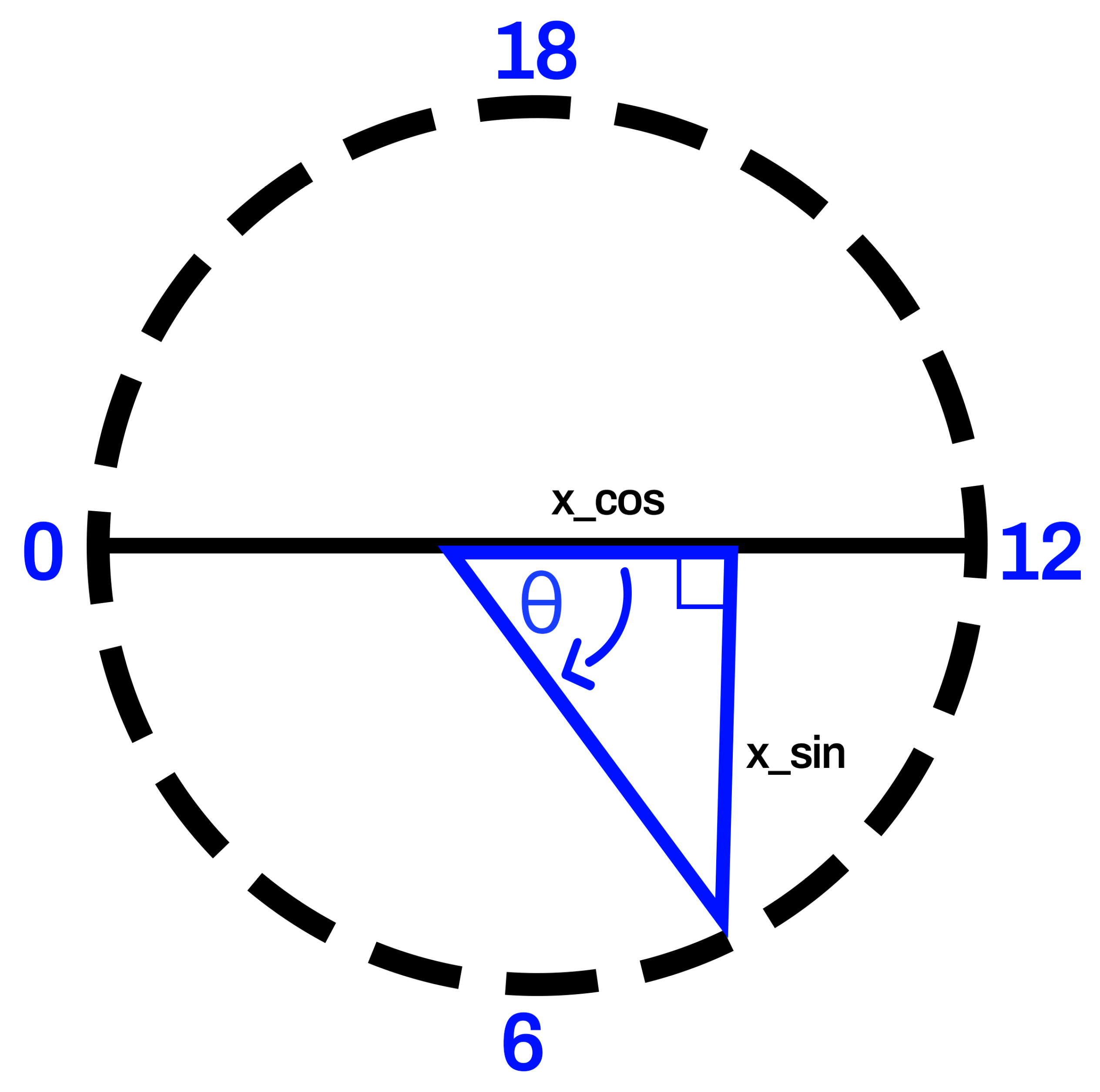
As shown in Figure 4, this study turns each time-related value (like day or month) into a circular format, so that the smallest and largest values sit next to each other. This is performed using sine and cosine functions, which allow us to represent time in a smooth, continuous way. In the example for hours, the circle starts at midnight on the left and moves counterclockwise. This means that 11:59 p.m. is placed right next to 12:00 a.m.—just like it is in real time. The same kind of transformation is applied to both the month and the day values in this study.

For days and months, the trigonometric cyclical transformation into sine and cosine components are expressed mathematically using Equation (1) and Equation (2), respectively.

$$x_{sin}=Sin(2\pi {\displaystyle \frac{x}{T}})$$

(1)

$$x_{cos}=Cos(2\pi {\displaystyle \frac{x}{T}})$$

(2)

where x is the cyclical feature value (e.g., month, day), T is the period of the cycle (e.g., 12 for months, 365 for days), $x_{sin}$ is the sine-transformed value, and $x_{cos}$ is the cosine-transformed value.

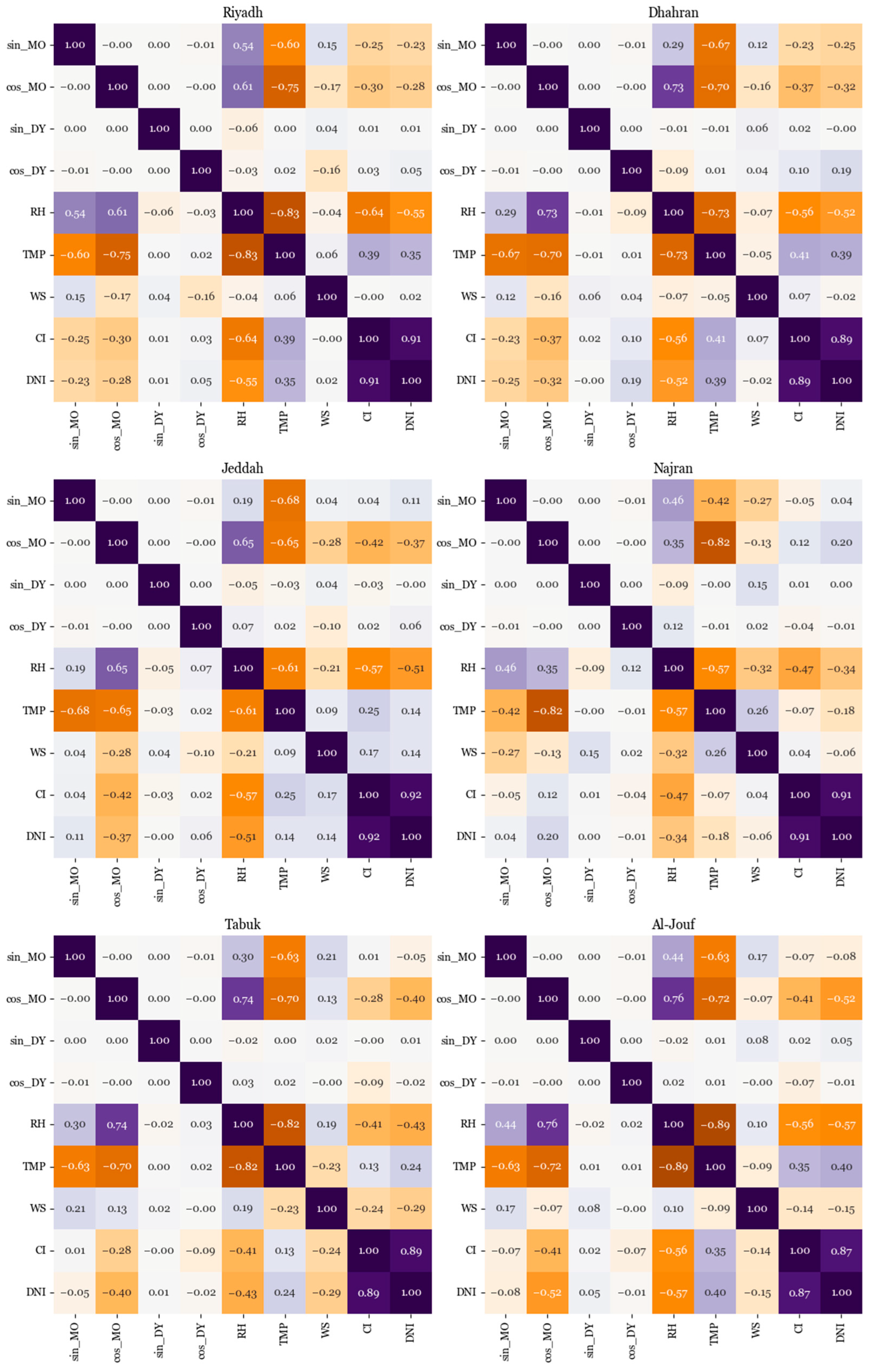
To better capture the seasonal patterns of solar radiation, TCE was applied to convert the temporal variables—month and day—into cosine and sine features to preserve the periodic nature of the time variables without introducing artificial breaks (for instance, between December and January). Figure 5 presents the correlation between the TCE features and the core climatic variables for each of the six case-study sites. Within Figure 5, clear seasonal signals are observed. For instance, in Riyadh, cos_month has a strong negative correlation with TMP (−0.75) and a positive correlation with RH (0.61). Similar relationships are visible in Dhahran, where cos_month correlates at −0.73 with TMP and 0.70 with RH. In Tabuk and Al-Jouf, which exhibit more extreme seasonal variability, sin_month and cos_month both maintain moderate correlations with DNI (up to −0.40. Also, the encoded features (sin_MO, cos_MO, sin_DY, and cos_DY) remain nearly uncorrelated with each other, demonstrating no clear redundancy or multicollinearity.

2.6. Performance Metrics

The performance metrics—MAE, MSE, RMSE, R², rRMSE, t-stat, MAPE, and MBE—were used to assess the performance of the ML models in this study. These metrics were carefully chosen to offer a thorough evaluation of the overall performance in estimating solar radiation, prediction accuracy, and error magnitude. An overview of the mathematical models of these metrics is presented in

Table 7. Mathematical models of performance metrics.

Metrics	Mathematical Model	Description	Desired Output
MAE	$MAE={\displaystyle \frac{1}{n}}{\displaystyle \sum _{i=1}^n}\left|y_i-{\widehat{y}}_i\right|$	Measures the mean magnitude of errors between predicted and actual values without considering their direction [49,50]	Closer to 0 is better
MSE	$MSE={\displaystyle \frac{1}{n}}{\displaystyle \sum _{i=1}^n}{\left(y_i-{\widehat{y}}_i\right)}^2$	Measures the mean squared differences between predicted and actual values, and penalises larger errors more heavily [49]	Closer to 0 is better
RMSE	$RMSE=\sqrt{{\displaystyle \frac{1}{n}}{\displaystyle \sum _{i=1}^n}{\left(y_i-{\widehat{y}}_i\right)}^2}$	Square root of MSE, providing error measure in the same units as the target variable [51]	Closer to 0 is better
${\mathrm{R}}^2$	$R^2=1-\left[{\displaystyle \frac{\sum {\left(y_i-{\widehat{y}}_i\right)}^2}{\sum {\left(y_i-{\overline{y}}_i\right)}^2}}\right]$	Explains the variation in the target variable that is predictable from the input variable(s) [52]	Closer to 1 is better
MAPE	$MAPE={\displaystyle \frac{1}{n}}{\displaystyle \sum _{i=1}^n}\left|{\displaystyle \frac{y_i-{\widehat{y}}_i}{y_i}}\right|\times 100$	Expresses accuracy as a percentage, showing the mean absolute percent difference between predicted and actual values [51,53]	Closer to 0% is better
MBE	$MBE={\displaystyle \frac{1}{n}}{\displaystyle \sum _{i=1}^n}\left({\widehat{y}}_i-y_i\right)$	Used to evaluate the bias of forecasting models [54]	Closer to 0 is better
rRMSE	$rRMSE={\displaystyle \frac{\sqrt{\frac{1}{n}{\sum }_{i=1}^n{\left(y_i-{\widehat{y}}_i\right)}^2}}{{\overline{y}}_i}}\times 100$	Derived from RMSE [51]	Closer to 0% is better

. Within Table 7, the term $y_i$ represents the actual observed values of the dependent variable, ${\widehat{y}}_i$ represents the predicted values from the ML models, $n$ denotes the number of observations, and ${\overline{y}}_i$ represents the mean of the actual observed values.

3. Results

3.1. Temporal Patterns of DNI and Climatic Variables

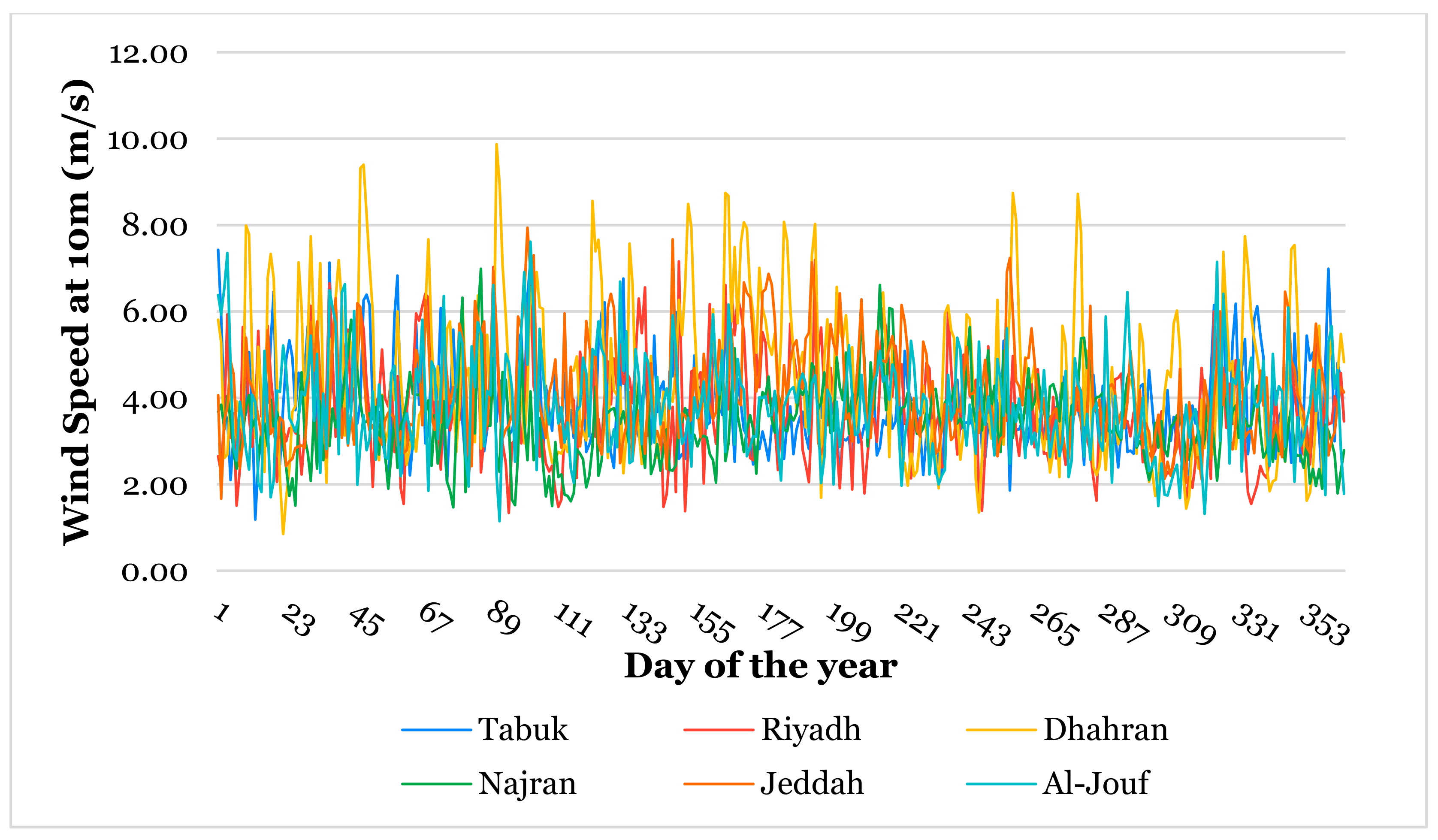
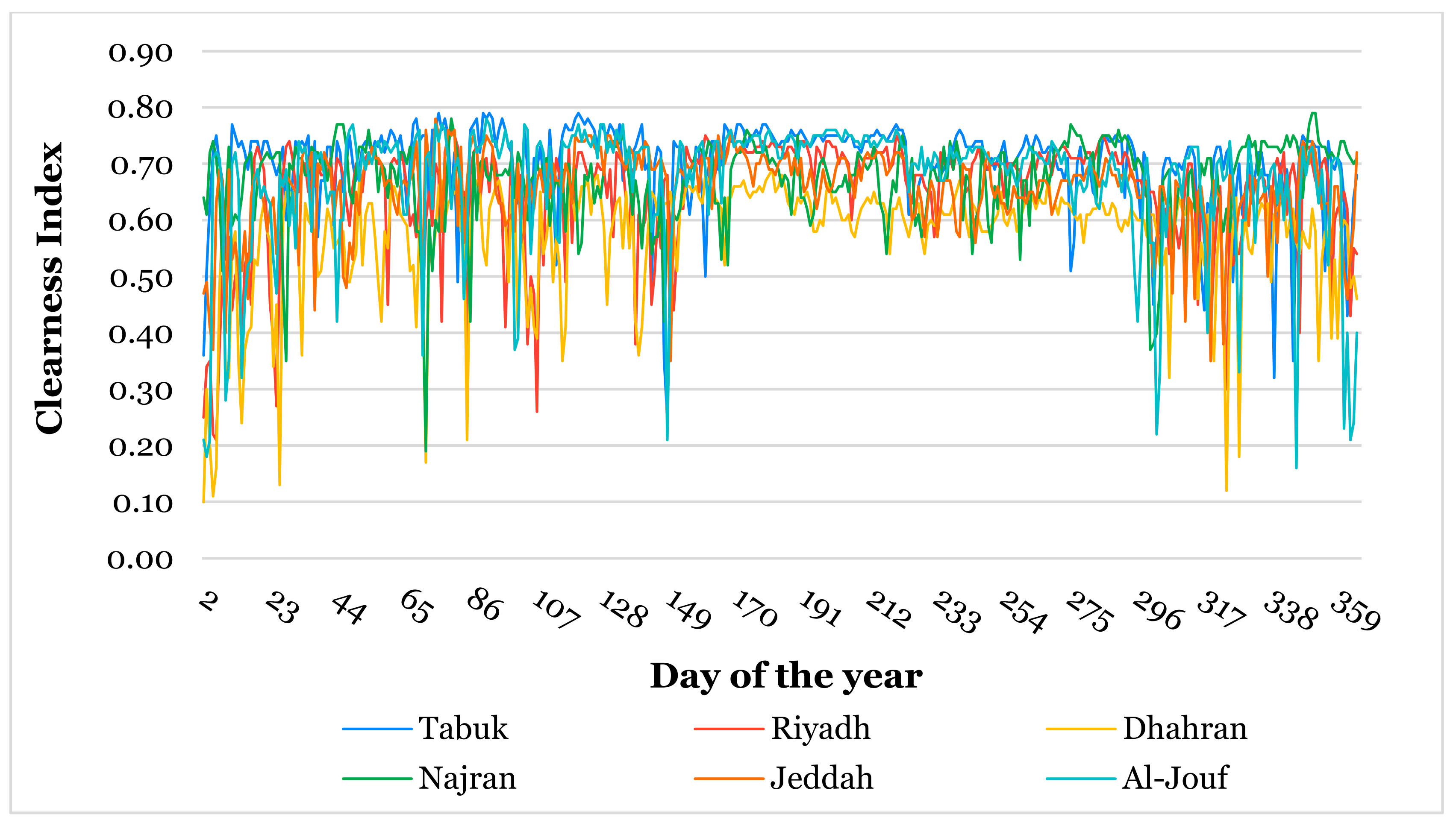
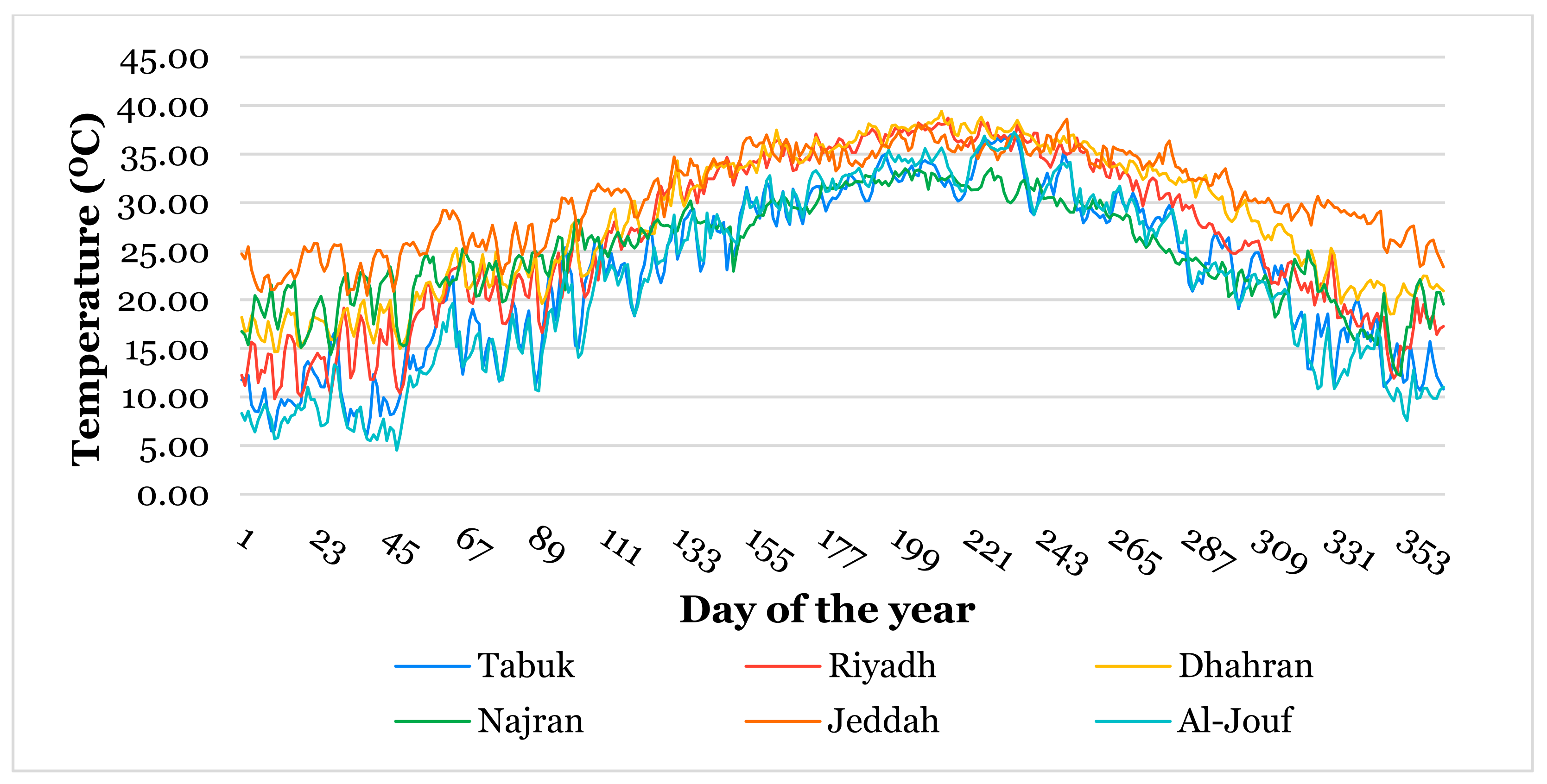
Accurate forecasting of solar radiation relies on a clear understanding of the local climatic dynamics influencing irradiance levels. This study identifies seasonal patterns and site-specific environmental behaviours that shape irradiance profiles and potentially affect ML model accuracy. Figure 6, Figure 7, Figure 8, Figure 9 and Figure 10 present the trends associated with DNI, WS, CI, RH, and TMP, respectively, providing a context for understanding the forecasting challenges and regional variations present across the study locations.

DNI in Tabuk consistently shows high values, particularly during the summer months (June–September), where it frequently reaches 8–10 kWh/m²/day, with noticeable dips during winter. Riyadh exhibits moderate variability, with values typically ranging from 3 to 7 kWh/m²/day and occasionally peaking above 8 kWh/m²/day during the summer months. Dhahran shows the most moderate profile among all cities, generally maintaining values between 2 and 5 kWh/m²/day, with some peaks reaching 6 kWh/m²/day during summer. Najran demonstrates considerable fluctuation throughout the year, with values ranging from 2 to 8 kWh/m²/day. Jeddah presents a relatively stable profile, with most values lying between 4 and 8 kWh/m²/day, though it experiences some significant spikes reaching up to 10 kWh/m²/day during certain periods. Al-Jouf shows a pattern somewhat similar to Tabuk, with high summer values often exceeding 8 kWh/m²/day, but exhibits more pronounced fluctuations during winter months, in which values can drop below 1 kWh/m²/day.

In terms of WS, Dhahran exhibits the most dynamic wind patterns at 10 m above ground level, with notable peaks reaching around 9 m/s during certain periods, and particularly showing stronger winds mid-year. Jeddah demonstrates relatively consistent moderate winds throughout the year, though with occasional highs above 7 m/s. Tabuk’s wind profile shows moderate variability, with speeds typically ranging between 2 and 7 m/s and some pronounced peaks in the early and later parts of the year. Riyadh experiences steady winds with occasional surges above 6 m/s, but generally maintains moderate speeds around 3–4 m/s. Al-Jouf presents a somewhat erratic pattern, with notable fluctuations between 2 and 7 m/s throughout the year. Najran maintains the most stable wind profile among all the studied sites, with speeds generally staying between 2 and 5 m/s, and fewer extreme variations.

Tabuk generally maintains higher and more stable CI values, often above 0.70, particularly during the middle months of the year, while experiencing some dips during the winter months. Riyadh shows moderate variability, with values typically ranging between 0.60 and 0.70, with occasional fluctuations below 0.50 during certain periods. Dhahran exhibits the most variable pattern among all cities, with notable drops in clearness during certain periods, sometimes falling below 0.20, but also reaching above 0.60. Najran demonstrates relatively consistent high clearness values, often above 0.65, with some lows near the end of the year. Jeddah shows moderate stability, with values generally varying between 0.60 and 0.70. Al-Jouf presents an interesting pattern with generally high clearness values, similar to Tabuk, but with more pronounced fluctuations during the winter months, when values can drop significantly below 0.40.

Dhahran and Jeddah maintain relatively stable RH levels, typically ranging between 50 and 70%, with Dhahran showing slightly higher summer values and Jeddah experiencing more consistent levels due to its coastal location. Al-Jouf and Tabuk demonstrate more pronounced variations, with higher humidity in winter months (reaching 80–85%) and lower levels during summer (dropping to 15–20%). Riyadh exhibits a similar pattern, but with less extreme fluctuations, showing higher humidity in winter (60–70%) and drier conditions in summer (15–30%). Najran presents the most variable pattern, with sharp transitions between seasons—experiencing very low humidity in early summer (below 20%) but reaching peaks of 70–75% during the winter months. There is a noticeable trend in which the inland cities (Riyadh, Najran) show more extreme humidity variations compared to coastal areas (Jeddah, Dhahran), while the northern cities (Al-Jouf, Tabuk) display strong seasonal patterns.

Jeddah maintains consistently high temperatures throughout the year, ranging from around 23 °C to 38 °C, with the least seasonal variation among all cities. Dhahran experiences more pronounced seasonal changes, with summer mean temperatures reaching up to 39 °C and winter values around 14 °C. Riyadh shows significant seasonal fluctuation, with summer peaks approaching 38 °C and winter temperatures dropping to around 11 °C. Najran demonstrates a moderate temperature profile, with summer highs near 33 °C and winter lows around 12 °C. Al-Jouf exhibits the most extreme seasonal variation, with temperatures ranging from as low as 5 °C in winter to around 37 °C in summer. Tabuk shows seasonal patterns similar to those of Al-Jouf but with slightly milder extremes, ranging from about 8 °C to 37 °C.

3.2. Model Performance Evaluation

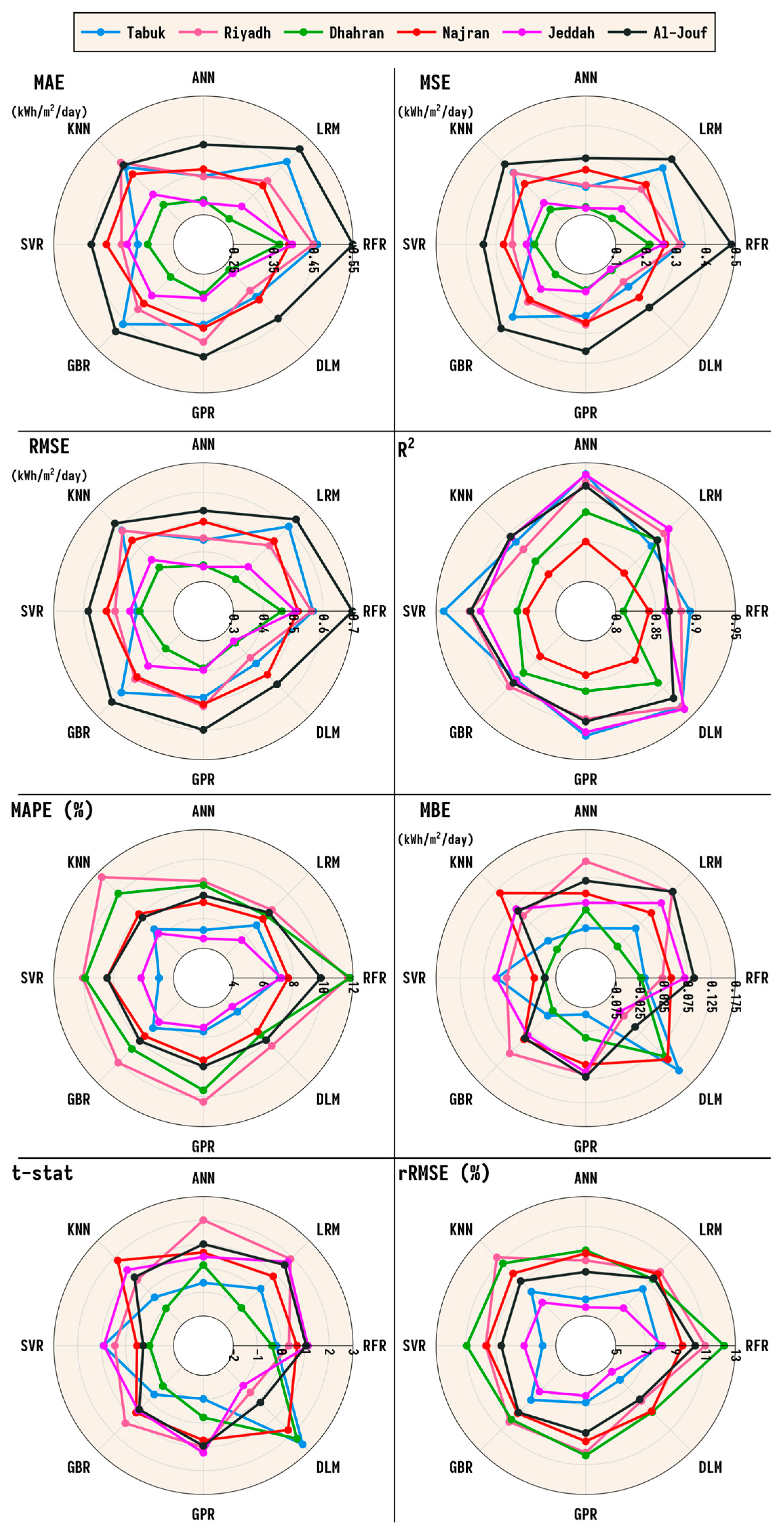
Figure 11 presents the performance comparison of eight ML algorithms across six distinct climatic regions in the KSA. Within Figure 11, a multi-metric and site-specific perspective on how each algorithm performs across the different regions is presented to capture central tendencies, trends, trade-offs, and variability in model behaviour. Previous studies have shown that non-ML formulations generally achieve RMSE values between 0.8 and 1.2 kWh/m²/day and R² below 0.85 in arid or semi-arid regions [13,52,54]. However, the proposed ML methods in this paper achieved substantially lower RMSE (0.343 kWh/m²/day) and higher R² (>0.93).

3.2.1. Multi-Metric Evaluation

In terms of MAE, models exhibit consistent variation across sites. The RFR notably records the highest MAE values across most locations, peaking in Al-Jouf at 0.549 and Riyadh at 0.450, while ANN and DNN models show relatively lower MAE values—ANN scoring 0.346 in Riyadh and DNN achieving 0.266 in Dhahran. A similar trend holds for MSE and RMSE—in which RFR again demonstrates relatively poor performance, particularly in Al-Jouf (MSE: 0.487, RMSE: 0.698), whereas DNN and ANN maintain high accuracy, especially in Dhahran and Jeddah, where DNN achieves RMSE values as low as 0.350 and 0.343, respectively. Regarding R², the DNN model maintains high performance across all sites, reaching 0.937 in Jeddah and 0.933 in Riyadh. ANN similarly performs well, particularly in Tabuk (0.936) and Jeddah (0.935). However, models like KNN and GBR show relatively reduced R² values, with KNN reaching a low of 0.828 in Najran, while the lowest recorded value for RFR was associated with Dhahran (0.809). SVR recorded the highest R² value, 0.941, in Tabuk. Now, regarding MAPE, performance diverges more sharply. RFR and KNN reported the highest MAPE values in several locations, such as Riyadh (RFR: 11.66%, KNN: 11.61%) and Dhahran (RFR: 11.81%, KNN: 10.04%), whereas DNN and ANN consistently scored below 10% across various sites, with the most outstanding performance by ANN being 4.65% at Jeddah. MBE values further differentiate model tendencies. ANN and DNN tended to show positive biases across most cities, such as 0.108 in Riyadh for ANN, while GPR and SVR exhibited lower or slightly negative biases for most sites. From the t-stat, values cluster around 1–2 for most models. Notably, ANN achieved a t-stat of 2.01 in Riyadh, while DNN achieved 2.28 and 2.62 in Dhahran and Tabuk, respectively. The rRMSE further validates DNN and ANN’s robustness, with values consistently below 9% across most sites. DNN reported the lowest rRMSE among the models and cities in Jeddah at 5.48%, while LRM, RFR, and KNN frequently exceeded 9%, particularly in Dhahran, Najran, and Al-Jouf.

3.2.2. Multi-Site Evaluation

In Riyadh, DNN registered the lowest RMSE, 0.4218 kWh/m²/day, and the highest R², 0.9334. DNN also showed the lowest rRMSE (8.25%) and a negative bias in MBE (−0.0248), indicating a slight underestimation. ANN closely followed, with an RMSE of 0.4462 and R² of 0.9255. While LRM showed a reasonable R² (0.9015), it produced a higher RMSE (0.5130) and the highest MBE (0.1176) thus far. The highest MAE (0.4676) and RMSE (0.5826) in Riyadh were associated with KNN, accompanied by an rRMSE of 11.40%. In Al-Jouf, ANN again produced the lowest RMSE, at 0.539, paired with the highest R², of 0.921. DNN closely matched this with an RMSE of 0.548 and R² of 0.918. SVR also performed well (RMSE: 0.585, R²: 0.907), but showed a higher MAPE (8.43%) against DNN (7.92%). RFR recorded the highest error values in this location, with an RMSE of 0.698 and an rRMSE of 10.32%. LRM and GBR also trailed behind, both exhibiting RMSE values above 0.63 and lower R² values under 0.90. In Dhahran, DNN once again recorded the lowest RMSE, at 0.3507, and the highest R², 0.8906. LRM showed competitive performance with an RMSE of 0.3523 and a lower MAPE (7.94%). GBR and ANN also performed similarly, with RMSEs of 0.378 and 0.355, respectively. SVR and KNN produced RMSEs above 0.40 and maintained moderate R² values of approximately 0.85. RFR displayed the least favourable outcome in this location, with the highest RMSE (0.4623), rRMSE (12.25%), and MAPE (11.81%). Jeddah exhibited favourable outcomes for DNN, which recorded the lowest RMSE (0.343), highest R² (0.937), and the lowest MAPE (4.73%). ANN delivered comparably strong results, with an RMSE of 0.349 and R² of 0.935. Both models achieved an rRMSE below 6%, outperforming RFR and KNN, which recorded RMSEs of 0.509 and 0.445, respectively. LRM offered a good R² of 0.909, but also an RMSE of 0.412 and MBE of 0.086, indicating a slight overprediction. GPR achieved a balanced performance, with an RMSE of 0.399 and R² of 0.915. In Najran, ANN yielded the lowest RMSE (0.502), MAE (0.365), and MAPE (7.10%). DNN and GPR followed, both with RMSE values less than 0.520 and R² values above 0.84. SVR showed slightly higher errors (RMSE: 0.524, MAPE: 8.44%), while GBR and LRM were similar in magnitude. RFR’s RMSE reached 0.516, along with an rRMSE of 9.47%, placing it among the higher-error models for this region. In Tabuk, SVR posted the lowest RMSE (0.4227) and highest R² (0.9405), with an MAE of 0.3394 and MAPE of 4.96%. ANN followed closely, achieving an RMSE of 0.4396 and R² of 0.9357. DNN’s RMSE was 0.449, slightly higher than the top performers, though it maintained a strong R² of 0.933. KNN, GBR, LRM and RFR were at the lower end of the performance spectrum at this site, with RMSEs above 0.56 and R² values below 0.89. GPR showed some promising performance, with an R² of 0.92 and MAPE of 5.62%.

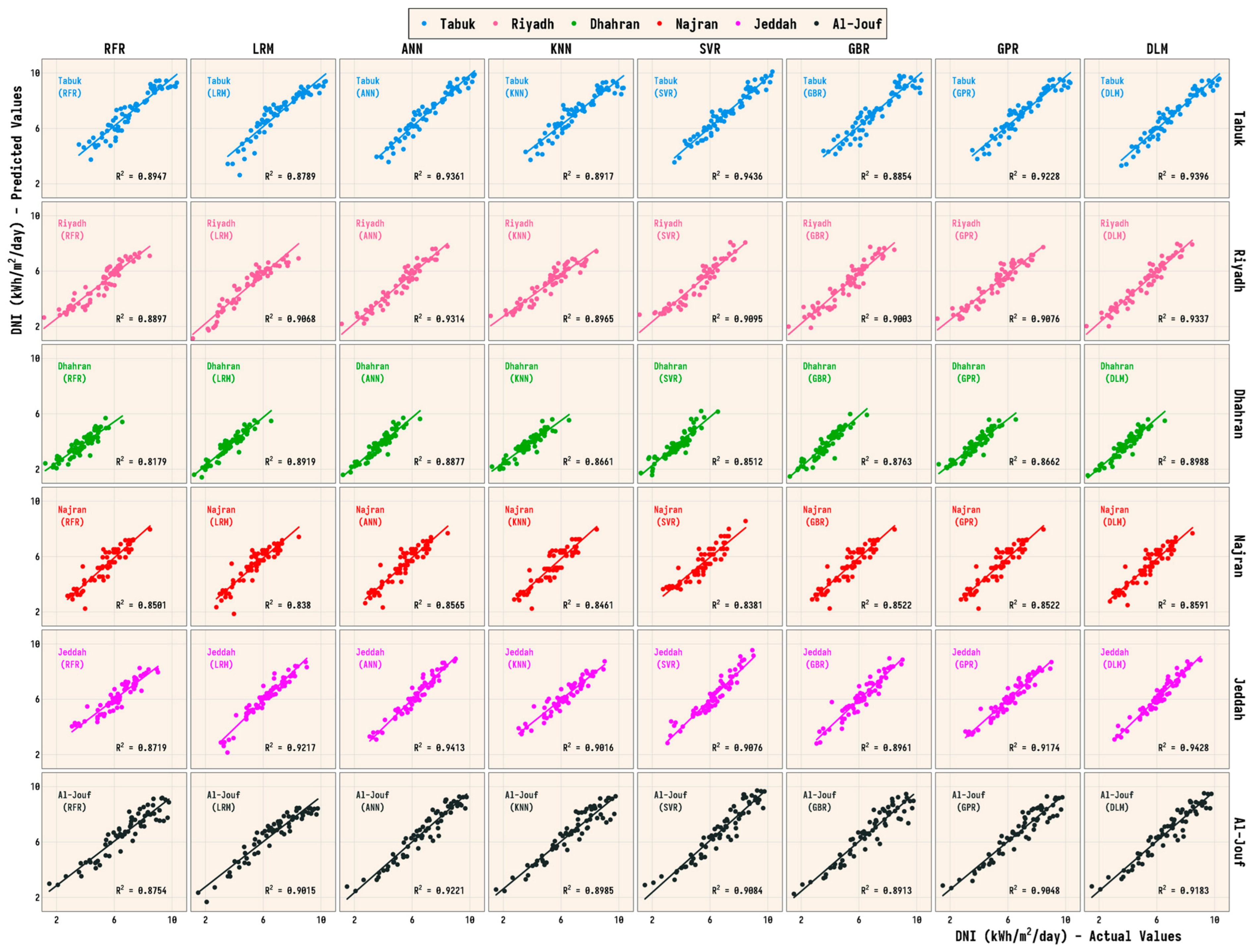
Figure 12 presents the models’ performance, with respect to the variation in our target variable (WS) explained by the models, for specific site–model combinations. Within Figure 12, ANN and DNN consistently demonstrate superior performance and near-perfect fits, with R² values exceeding 0.93 in Tabuk, Jeddah, and Dhahran. On the other hand, LRM and RFR yielded the lowest R² values and showed more scattered prediction patterns, particularly in Riyadh, Tabuk, and Najran. Also, ANN demonstrated the most consistently high R² scores across various sites, achieving an R² of 0.9361 in Tabuk, for instance. Similarly, in Jeddah and Al-Jouf, ANN attained R² values of 0.9413 and 0.9221, respectively. In Riyadh, ANN recorded an R² of 0.9314, SVR recorded 0.9095, and LRM showed some promise with 0.9068. DNN performed remarkably well, recording the highest R² in Jeddah at 0.9428, 0.9396 in Tabuk, 0.8988 in Dhahran, and 0.9337 in Riyadh, albeit its fitness to the actual values was slightly less tight in Najran (0.8591). SVR showed particularly strong performance in Tabuk (0.9436) and Riyadh (0.9095), closely rivalling or outperforming ANN and DNN in some instances. However, its R² dropped in Najran (0.8381) and Dhahran (0.8512). GBR and GPR both delivered moderately strong results—the former peaked in Riyadh (R² = 0.9083) and dropped in Najran (0.8522), while the latter maintained a relatively consistent performance across sites, scoring R² values between 0.8522 in Najran and 0.9228 in Tabuk. KNN demonstrated reasonably good fits in Jeddah (0.9016) and Dhahran (0.8661), but performance dipped slightly in Al-Jouf (0.8985) and Tabuk (0.8917). RFR delivered R² values above 0.85 in most cases but failed to exceed 0.90 consistently. Its highest performance was in Al-Jouf (0.8754) and Riyadh (0.8897), with noticeable scatters in sites like Dhahran (0.8179) and Najran (0.8501). LRM achieved unexpectedly high R² in Riyadh (0.9068) and Al-Jouf (0.9015) but saw some deviations from the regression line in sites like Tabuk (0.8789) and Najran (0.8380).

3.3. Temporal Performance Evaluation

In addition to overall fit (see Figure 12), the predictive capability of each algorithm was validated using a hold-out test set comprising 20% of the data (randomly selected from the full year). Figure 13 presents a comparative time-series prediction trend of predicted versus actual values. Within Figure 13, actual and predicted daily DNI values are plotted along with their corresponding absolute error trends.

In Tabuk, predictions exhibit consistent seasonal tracking across most models. ANN and SVR show relatively smooth alignment with observed values, with visibly lower absolute errors across the mid-year high-radiation months. However, LRM, RFR, and KNN display intermittent spikes in error, particularly around transitional periods like April and October. DNN maintains a generally close fit to the actual values across all months but reveals minor overprediction during the late summer period.

For Riyadh, models such as SVR and DNN demonstrate minimal divergence from actual values, especially during peak summer, when the atmospheric conditions are relatively stable. The absolute error plots for SVR in Riyadh remain compressed around the baseline throughout most of the year. On the other hand, LRM and KNN show pronounced error peaks between April and August.

In Dhahran, the predictive trajectories for DNN and ANN follow the actual DNI curve with considerable consistency, particularly from June through September. While GBR and GPR show generally stable performance, RFR again reveals sharp deviations during the transitional months. The absolute error plots reinforce these patterns, where ANN and DNN produce the narrowest error bands compared to other models.

Najran’s results highlight increased volatility in predictions across all models. KNN and LRM showed larger deviations between predicted and actual values during the second and fourth quarters of the year. ANN maintains relative proximity to observed values during high solar periods, but the frequent smaller oscillations in the absolute error trace indicate continuous minor prediction fluctuations.

In Jeddah, both ANN and DNN show close agreement with actual DNI values for much of the year. Their absolute error profiles remain suppressed throughout most of the year, notably from May to September. SVR and GBR also perform steadily but exhibit occasional surges in error, particularly during the brief cloudy intervals typical of coastal regions.

In Al-Jouf, the seasonal trend associated with DNI is more pronounced, with wider intra-annual variability. SVR and ANN show strong alignment during summer months but diverge slightly in the early part of the year. KNN and RFR exhibit broader, more erratic absolute error spikes throughout the time series, especially from January through March, and again in October.

3.4. Impact of Trigonometric Cyclical Encoding (TCE)

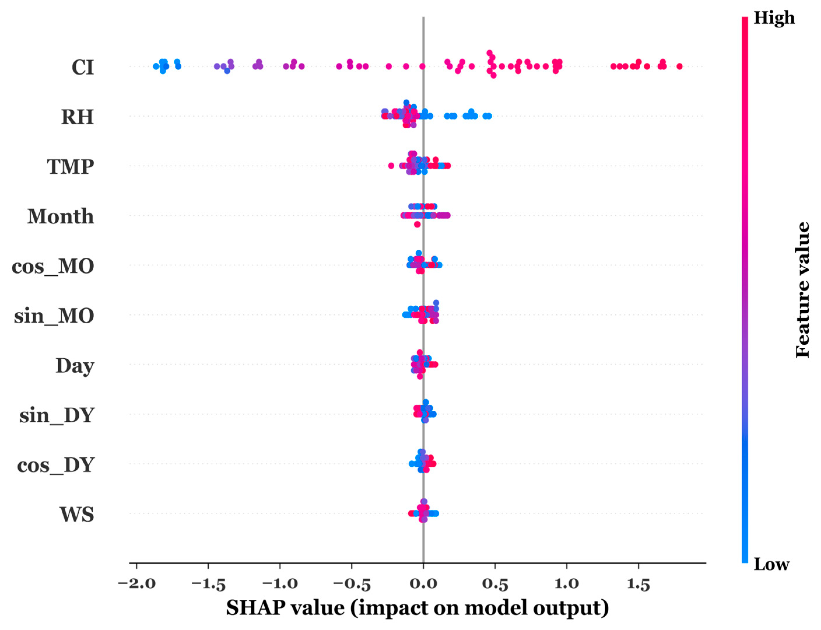
We conducted a comparative analysis of feature importance to quantitatively evaluate the efficacy of TCE. We analysed how TCE influences the explanatory power of temporal features. This was achieved by training two separate RFR models under identical conditions. The first model utilised raw-integer representations of temporal features (Month, Day), while the second model employed the cyclical encoded features (sin Month, cos Month, sin Day, and cos Day). The SHAP framework was then applied to both models to obtain a rigorous, consistent measure of each feature’s marginal contribution to the ML algorithm [55]. For a direct comparison, the sine and cosine components of each temporal concept were aggregated to represent the total importance of the Cyclical Month and Cyclical Day features. Figure 14 presents the SHAP summary plot for both models.

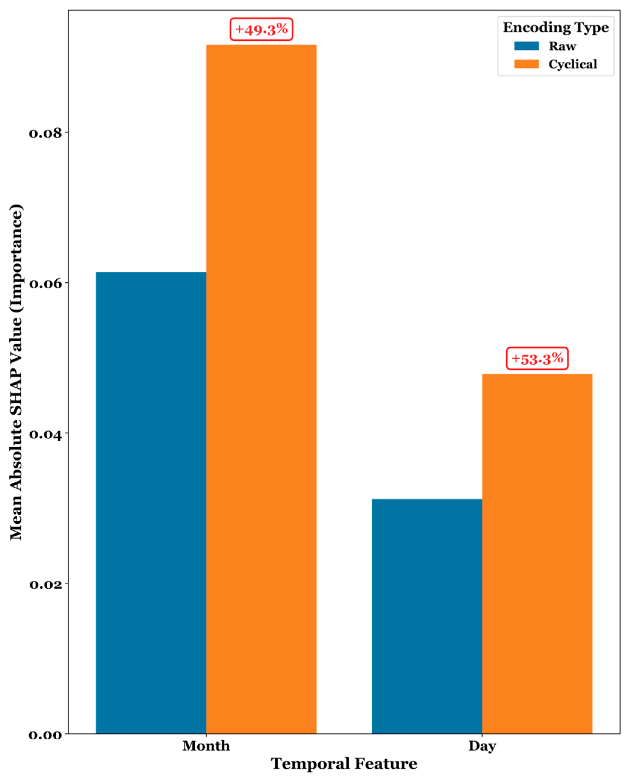
Figure 15 presents the quantitative comparison of raw features against the cyclically encoded features. Within Figure 15, the importance for the cyclically encoded features showed a significant increase over the raw features. The importance for the monthly cycle increased by 49.26%, while the importance for the daily cycle increased by 53.30%.

4. Conclusions

This study comprehensively evaluated the performance of eight ML models for forecasting solar radiation across six climatically diverse sites in Saudi Arabia. The models evaluated include RFR, LRM, ANN, KNN, SVR, GBR, GPR, and DNN. Eight statistical metrics were used to assess predictive accuracy and generalizability across each site. The key findings, derived from an extensive multi metric-site evaluation, are summarized as follows:

• The Deep Learning (DNN) and Artificial Neural Network (ANN) models demonstrated superior and consistent performance across most locations, with DNN achieving the lowest RMSE (as low as 0.343 kWh/m²/day, in Jeddah) and ANN showing remarkable stability and low error rates (e.g., an MAPE of 7.10% in Najran).
• Model effectiveness was significantly influenced by geographical and climatic conditions. Support Vector Regression (SVR) excelled in specific arid inland regions like Riyadh and Tabuk, while other models, such as RFR and KNN, exhibited greater performance volatility.
• The implementation of Trigonometric Cyclical Encoding (TCE) for temporal features substantially enhanced model learning. A comparative analysis revealed that TCE increased the feature importance of temporal signals by over 49% for monthly cycles and 53% for daily cycles, enabling models to more effectively capture fundamental periodic patterns in solar radiation.
• Time-series and error analyses confirmed that ANN and DNN maintained the most stable prediction accuracy, particularly during high solar radiation seasons, whereas other models showed wider fluctuations.

Limitations and Future Research

Although the dataset used in this study adequately captures short-term temporal and seasonal dynamics, it may not fully represent inter-annual climatic variability. Multi-year datasets could be used in future studies to capture long-term patterns and ensure better model robustness under diverse climatic fluctuations.

References

1. Margaritou, M.D.; Tzannatos, E. A multi-criteria optimization approach for solar energy and wind power technologies in shipping. FME Trans. 2018, 46, 374–380. [Google Scholar] [CrossRef]
2. Bezari, S.; Bekkouche, S.M.E.A.; Benchatti, A. Investigation and Improvement for a Solar Greenhouse Using Sensible Heat Storage Material. FME Trans. 2020, 49, 154–162. [Google Scholar] [CrossRef]
3. Rašuo, B.P.; Bengin, A.Č. Optimization of Wind Farm Layout. FME Trans. 2010, 38, 107–114. [Google Scholar]
4. Rashid, L.B.; Musah, A.; Amoah, R.K. Technoeconomic Feasibility of Renewable Energy Systems for Sporting Stadiums. Int. J. Energy Res. 2025, 2025, 9701161. [Google Scholar] [CrossRef]
5. Gojak, M.; Ljubinac, F.; Banjac, M. Simulation of solar water heating system. FME Trans. 2019, 47, 1–6. [Google Scholar] [CrossRef]
6. Rašuo, B.; Dinulović, M.; Veg, A.; Grbović, A.; Bengin, A. Harmonization of new wind turbine rotor blades development process: A review. Renew. Sustain. Energy Rev. 2014, 39, 874–882. [Google Scholar] [CrossRef]
7. Parezanovic, V.; Rasuo, B.; Adzic, M. Design of Airfoils for Wind Turbine Blades. 2006, 17–24. Available online: https://www.researchgate.net/publication/228608628_DESIGN_OF_AIRFOILS_FOR_WIND_TURBINE_BLADES (accessed on 18 June 2025).
8. Stojicevic, M.; Jeli, Z.; Obradovic, M.; Obradovic, R.; Marinescu, G.C. Designs of solar concentrators. FME Trans. 2019, 47, 273–278. [Google Scholar] [CrossRef]
9. Hussain, F.M.; Rehman, S.; Al-Sulaiman, F.A. Performance Analysis of a Solar Chimney Power Plant for Different Geographical Locations of Saudi Arabia. FME Trans. 2020, 49, 64–71. [Google Scholar] [CrossRef]
10. Habtay, G.; Buzas, J.; Farkas, I. Heat Transfer analysis in the chimney of the indirect solar dryer under natural convection mode. FME Trans. 2020, 48, 701–706. [Google Scholar] [CrossRef]
11. Jakoplić, A.; Franković, D.; Kirinčić, V.; Plavšić, T. Benefits of short-term photovoltaic power production forecasting to the power system. Optim. Eng. 2021, 22, 9–27. [Google Scholar] [CrossRef]
12. Qing, X.; Niu, Y. Hourly day-ahead solar irradiance prediction using weather forecasts by LSTM. Energy 2018, 148, 461–468. [Google Scholar] [CrossRef]
13. Bayrakçı, H.C.; Demircan, C.; Keçebaş, A. The development of empirical models for estimating global solar radiation on horizontal surface: A case study. Renew. Sustain. Energy Rev. 2018, 81, 2771–2782. [Google Scholar] [CrossRef]
14. Hissou, H.; Benkirane, S.; Guezzaz, A.; Azrour, M.; Beni-Hssane, A. A Novel Machine Learning Approach for Solar Radiation Estimation. Sustainability 2023, 15, 10609. [Google Scholar] [CrossRef]
15. Solano, E.S.; Affonso, C.M. Solar Irradiation Forecasting Using Ensemble Voting Based on Machine Learning Algorithms. Sustainability 2023, 15, 7943. [Google Scholar] [CrossRef]
16. Rehman, S.; Salman, U.T.; Mohandes, M.A.; Al-Sulaiman, F.A.; Adetona, S.; Alhems, L.M.; Baseer, M.A. Wind Speed Prediction Based on Long-Short Term Memory using Nonlinear Autoregressive Neural Networks. FME Trans. 2022, 50, 260–270. [Google Scholar] [CrossRef]
17. Rehman, S.; Khan, S.A.; Alhems, L.M. The Effect of Acceleration Coefficients in Particle Swarm Optimization Algorithm with Application to Wind Farm Layout Design. FME Trans. 2020, 48, 922–930. [Google Scholar] [CrossRef]
18. Mohandes, M.; Nuha, H.H.; Mugitama, S.A.; Rehman, S.; Al-Shailkhi, A. Global solar radiation prediction using machine learning approaches. Sigma J. Eng. Nat. Sci.—Sigma Mühendislik Ve Fen Bilim. Derg. 2025, 43, 1725–1736. [Google Scholar] [CrossRef]
19. Chaibi, M.; Benghoulam, E.M.; Tarik, L.; Berrada, M.; El Hmaidi, A. Machine Learning Models Based on Random Forest Feature Selection and Bayesian Optimization for Predicting Daily Global Solar Radiation. Int. J. Renew. Energy Dev. 2022, 11, 309–323. [Google Scholar] [CrossRef]
20. Bakır, H. Prediction of daily global solar radiation in different climatic conditions using metaheuristic search algorithms: A case study from Türkiye. Environ. Sci. Pollut. Res. 2024, 31, 43211–43237. [Google Scholar] [CrossRef]
21. Lu, Y.; Wang, L.; Zhu, C.; Zou, L.; Zhang, M.; Feng, L.; Cao, Q. Predicting surface solar radiation using a hybrid radiative Transfer–Machine learning model. Renew. Sustain. Energy Rev. 2023, 173, 113105. [Google Scholar] [CrossRef]
22. Khafaga, D.S.; Alhussan, A.A.; Eid, M.M.; El-kenawy, E.-S.M. Improving solar radiation source efficiency using adaptive dynamic squirrel search optimization algorithm and long short-term memory. Front. Energy Res. 2023, 11, 1164528. [Google Scholar] [CrossRef]
23. Zell, E.; Gasim, S.; Wilcox, S.; Katamoura, S.; Stoffel, T.; Shibli, H.; Engel-Cox, J.; Al Subie, M. Assessment of solar radiation resources in Saudi Arabia. Sol. Energy 2015, 119, 422–438. [Google Scholar] [CrossRef]
24. Mohandes, M.; Khan, S.A.; Rehman, S.; Al-Shaikhi, A.; Liu, B.; Iqbal, K. GARM: A Stochastic Evolution based Genetic Algorithm with Rewarding Mechanism for Wind Farm Layout Optimization. FME Trans. 2023, 51, 575–584. [Google Scholar] [CrossRef]
25. Živković, G.S.; Mirkov, N.S.; Dakić, D.V.; Erić, A.M.; Erić, M.D.; Rudonja, N.R. Numerical Simulation of Thermo-Fluid Properties and Optimisation of Hot Water Storage Tank in Biomass Heating Systems. FME Trans. 2010, 38, 63–70. [Google Scholar]
26. Nadeem, T.B.; Ali, S.U.; Asif, M.; Suberi, H.K. Forecasting daily solar radiation: An evaluation and comparison of machine learning algorithms. AIP Adv. 2024, 14, 75010. [Google Scholar] [CrossRef]
27. Hossain, M.K.; Arifuzzaman, M.; Seliaman, M.E.; Rahman, A.; Sarker, D.; Altammar, H. Ensemble Learning Algorithms for Solar Power Prediction in Saudi Arabia: A Data-Driven Approach. In Proceedings of the 2024 ASU International Conference in Emerging Technologies for Sustainability and Intelligent Systems (ICETSIS), Manama, Bahrain, 28–29 January 2024; pp. 1368–1372. [Google Scholar] [CrossRef]
28. Hissou, H.; Benkirane, S.; Guezzaz, A.; Beni-Hssane, A.; Azrour, M. Advanced Prediction of Solar Radiation Using Machine Learning and Principal Component Analysis; Springer: Cham, Switzerland, 2024; pp. 201–207. [Google Scholar] [CrossRef]
29. Villegas-Mier, C.; Rodriguez-Resendiz, J.; Álvarez-Alvarado, J.; Jiménez-Hernández, H.; Odry, Á. Optimized Random Forest for Solar Radiation Prediction Using Sunshine Hours. Micromachines 2022, 13, 1406. [Google Scholar] [CrossRef]
30. Wang, S.; Ma, J. A novel GBDT-BiLSTM hybrid model on improving day-ahead photovoltaic prediction. Sci. Rep. 2023, 13, 15113. [Google Scholar] [CrossRef]
31. Duan, J.; Zuo, H.; Bai, Y.; Chang, M.; Chen, X.; Wang, W.; Ma, L.; Chen, B. A multistep short-term solar radiation forecasting model using fully convolutional neural networks and chaotic aquila optimization combining WRF-Solar model results. Energy 2023, 271, 126980. [Google Scholar] [CrossRef]
32. Rehman, S.; Mohandes, M. Splitting Global Solar Radiation into Diffuse and Direct Normal Fractions Using Artificial Neural Networks. Energy Sources Part A Recovery Util. Environ. Eff. 2012, 34, 1326–1336. [Google Scholar] [CrossRef]
33. Tercha, W.; Tadjer, S.A.; Chekired, F.; Canale, L. Machine Learning-Based Forecasting of Temperature and Solar Irradiance for Photovoltaic Systems. Energies 2024, 17, 1124. [Google Scholar] [CrossRef]
34. Dikmen, O. Predicting Solar Irradiance Using Machine Learning Approaches: The Case of Duzce, Turkey. Int. J. Adv. Nat. Sci. Eng. Res. 2024, 8, 133–145. [Google Scholar]
35. Soleymani, S.; Mohammadzadeh, S. Comparative Analysis of Machine Learning Algorithms for Solar Irradiance Forecasting in Smart Grids. arXiv 2023, arXiv:2310.13791. [Google Scholar] [CrossRef]
36. Mohandes, M.; Balghonaim, A.; Kassas, M.; Rehman, S.; Halawani, T.O. Use of radial basis functions for estimating monthly mean daily solar radiation. Sol. Energy 2000, 68, 161–168. [Google Scholar] [CrossRef]
37. Rasuo, B.P.; Veg, A.D. Design, fabrication and verification testing of the wind turbine rotor blades from composite materials. In Proceedings of the ICCM International Conferences on Composite Materials, Kyoto, Japan, 9–13 July 2007; pp. 1–4. [Google Scholar]
38. Dinulovic, M.; Trninic, M.; Rasuo, B.; Kozovic, D. Methodology for aeroacoustic noise analysis of 3-bladed h-Darrieus wind turbine. Therm. Sci. 2023, 27, 61–69. [Google Scholar] [CrossRef]
39. Rašuo, B.; Bengin, A.; Veg, A. On Aerodynamic Optimization of Wind Farm Layout. Proc. Appl. Math. Mech. 2010, 10, 539–540. [Google Scholar] [CrossRef]
40. Mousavi, S.S.; Schukat, M.; Howley, E. Deep Reinforcement Learning: An Overview. In Proceedings of the SAI Intelligent Systems Conference (IntelliSys) 2016, London, UK, 21–22 September 2016; pp. 426–440. [Google Scholar] [CrossRef]
41. Rohanian, O.; Jauncey, H.; Nouriborji, M.; Kumar, V.; Gonalves, B.P.; Kartsonaki, C.; Isaric Clinical Characterisation Group; Merson, L.; Clifton, D. Using Bottleneck Adapters to Identify Cancer in Clinical Notes under Low-Resource Constraints. arXiv 2022, arXiv:2210.09440. [Google Scholar] [CrossRef]
42. Alabdulhadi, A.A.; Rehman, S.; Ali, A.; Shafiullah, M. Deep learning framework for wind speed prediction in Saudi Arabia. Neural. Comput. Appl. 2025, 37, 3685–3701. [Google Scholar] [CrossRef]
43. Rehman, S.; Mohandes, M. Artificial neural network estimation of global solar radiation using air temperature and relative humidity. Energy Policy 2008, 36, 571–576. [Google Scholar] [CrossRef]
44. Chauhan, V.K.; Zhou, J.; Lu, P.; Molaei, S.; Clifton, D.A. A brief review of hypernetworks in deep learning. Artif. Intell. Rev. 2024, 57, 250. [Google Scholar] [CrossRef]
45. Uçak, K.; Günel, G.Ö. Adaptive stable backstepping controller based on support vector regression for nonlinear systems. Eng. Appl. Artif. Intell. 2024, 129, 107533. [Google Scholar] [CrossRef]
46. Tahir, M.F.; Yousaf, M.Z.; Tzes, A.; El Moursi, M.S.; El-Fouly, T.H.M. Enhanced solar photovoltaic power prediction using diverse machine learning algorithms with hyperparameter optimization. Renew. Sustain. Energy Rev. 2024, 200, 114581. [Google Scholar] [CrossRef]
47. Young, S.R.; Rose, D.C.; Karnowski, T.P.; Lim, S.-H.; Patton, R.M. Optimizing deep learning hyper-parameters through an evolutionary algorithm. In Proceedings of the Workshop on Machine Learning in High-Performance Computing Environments, Austin, TX, USA, 15 November 2015; pp. 1–5. [Google Scholar] [CrossRef]
48. Gurenko, V.V.; Bychkov, B.I.; Syuzev, V.V. An Approach to Simulation of Stationary and Non-stationary Processes in the Harmonic Basis. In Proceedings of the 2021 IEEE Conference of Russian Young Researchers in Electrical and Electronic Engineering (ElConRus), St. Petersburg, Moscow, Russia, 26–29 January 2021; pp. 2664–2667. [Google Scholar] [CrossRef]
49. Shcherbakov, M.V.; Brebels, A.; Shcherbakova, N.L.; Tyukov, A.P.; Janovsky, T.A.; Kamaev, V.A. A Survey of Forecast Error Measures. World Appl. Sci. J. 2013, 24, 171–176. [Google Scholar] [CrossRef]
50. Chen, C.; Twycross, J.; Garibaldi, J.M. A new accuracy measure based on bounded relative error for time series forecasting. PLoS ONE 2017, 12, e0174202. [Google Scholar] [CrossRef] [PubMed]
51. Zang, H.; Cheng, L.; Ding, T.; Cheung, K.W.; Wang, M.; Wei, Z.; Sun, G. Application of functional deep belief network for estimating daily global solar radiation: A case study in China. Energy 2020, 191, 116502. [Google Scholar] [CrossRef]
52. Yang, L.; Cao, Q.; Yu, Y.; Liu, Y. Comparison of daily diffuse radiation models in regions of China without solar radiation measurement. Energy 2020, 191, 116571. [Google Scholar] [CrossRef]
53. Gouda, S.G.; Hussein, Z.; Luo, S.; Yuan, Q. Model selection for accurate daily global solar radiation prediction in China. J. Clean. Prod. 2019, 221, 132–144. [Google Scholar] [CrossRef]
54. Fan, J.; Wang, X.; Wu, L.; Zhang, F.; Bai, H.; Lu, X.; Xiang, Y. New combined models for estimating daily global solar radiation based on sunshine duration in humid regions: A case study in South China. Energy Convers. Manag. 2018, 156, 618–625. [Google Scholar] [CrossRef]
55. Petrosian, O.; Zhang, Y. Solar Power Generation Forecasting in Smart Cities and Explanation Based on Explainable AI. Smart Cities 2024, 7, 3388–3411. [Google Scholar] [CrossRef]
Figure 1. Methodological flowchart.
Forecasting 07 00058 g001
Figure 2. Geographical distribution of case-study sites across Saudi Arabia (Source: the Authors).
Forecasting 07 00058 g002
Figure 3. DNI resource map of the KSA (Source: Solargis).
Forecasting 07 00058 g003
Figure 4. Cyclical features (Source: the Authors).
Forecasting 07 00058 g004
Figure 5. Correlation of TCE Features and climatic variables across the six case-study sites.
Forecasting 07 00058 g005
Figure 6. DNI trends across cities.
Forecasting 07 00058 g006
Figure 7. WS trends across cities.
Forecasting 07 00058 g007
Figure 8. CI trends across cities.
Forecasting 07 00058 g008
Figure 9. RH trends across cities.
Forecasting 07 00058 g009
Figure 10. TMP trends across cities.
Forecasting 07 00058 g010
Figure 11. Multi-metric performance across sites.
Forecasting 07 00058 g011
Figure 12. Actual vs. predicted DNI across sites and models.
Forecasting 07 00058 g012
Figure 13. Prediction patterns and absolute error trends, based on the 20% of unseen test data.
Forecasting 07 00058 g013
Figure 14. Comparison of SHAP summary of cyclically encoded features and raw features.
Forecasting 07 00058 g014
Figure 15. Comparison of aggregated SHAP importance for raw versus cyclically encoded temporal features.
Forecasting 07 00058 g015