Article

Comparison of Linear and Beta Autoregressive Models in Forecasting Nonstationary Percentage Time Series

by
Carlo Grillenzoni
IUAV: Institute of Architecture, University of Venice, St Croce, n. 1957, 30135 Venezia, Italy
Forecasting 2025, 7(4), 57; https://doi.org/10.3390/forecast7040057
Submission received: 9 September 2025 / Revised: 7 October 2025 / Accepted: 9 October 2025 / Published: 13 October 2025
(This article belongs to the Special Issue Feature Papers of Forecasting 2025)

Abstract

Positive percentage time series are present in many empirical applications; they take values in the continuous interval (0,1) and are often modeled with linear dynamic models. Risks of biased predictions (outside the admissible range) and problems of heteroskedasticity in the presence of asymmetric distributions are ignored by practitioners. Alternative models are proposed in the statistical literature; the most suitable is the dynamic beta regression which belongs to generalized linear models (GLM) and uses the logit transformation as a link function. However, owing to the Jensen inequality, this approach may also not be optimal in prediction; thus, the aim of the present paper is the in-depth forecasting comparison of linear and beta autoregressions. Simulation experiments and applications to nonstationary time series (the US unemployment rate and BR hydroelectric energy) are carried out. Rolling regression for time-varying parameters is applied to both linear and beta models, and a prediction criterion for the joint selection of model order and sample size is defined.

1. Introduction

In time series analysis, one may often encounter positive percentage data, i.e., data that fall in the open interval (0,1). Examples include the unemployment rate in economics [1], plant utilization in engineering [2], drought index in ecology [3], crime rates in sociology [4] and infection spread in epidemiology [5]. Despite the fact that these data violate the assumption of Gaussianity and often have strong asymmetric distributions, they are usually fitted with linear dynamic models; e.g., [6]. This approach involves the risk of bias in the forecasts (if they are outside the admissible range) and bias in the tests of causality with other series. Indeed, as the response variable approaches the boundaries, its variance shrinks and the implied models become heteroskedastic. This, in turn, involves inefficient parameter estimates with biased standard errors, which affect confidence intervals and test statistics.
To avoid these problems, the statistical literature has proposed various solutions; the simplest is to transform the data with log-based functions to have unbounded codomains, and then fit the resulting series with linear models [7]. More technical approaches intervene on the structure of the systems, by controlling the parameter values with constrained least squares (LS) [8]; or by modeling the response variable with bounded support densities (mainly of the beta family) and various models [9], and parameter estimation is performed using maximum likelihood (ML) [10]. This approach involves iterative algorithms, which easily converge if the likelihood is unimodal; however, their iterative nature hinders the application of recursive methods for nonstationary data (e.g., the Kalman filter) [11].
For stationary time series, beta regression is the best-known method [9] and has been extended to dynamic models by [12,13]. It belongs to generalized linear models (GLMs), which adopt link functions to connect the response variable to the regression function. The preferred link of the beta regression is the logit one, typically adopted in binary response models; its usage in the percentage data can be seen as the attempt to project the response variable on the real line ± and/or the regression function in the interval (0,1). However, data transformations involve issues of coefficient interpretation [14] and loss of optimality in forecasting; in fact, owing to the Jensen inequality, the expectation of a transformation is different from the transformation of the expectation.
Given this scenario, in this paper, we will compare the forecasting performance of standard linear models and beta dynamic regression, applied to two monthly series: the unemployment rate in the US [1,6] and the hydroelectric energy storage in BR [13]. In the statistical literature there are no such comparisons, and our evaluation is carried out in-depth, on wide out-of-sample periods and long-range prediction intervals. The analysis is restricted to autoregressive (AR) models in view of their long-range forecasting ability; we find that there are not significant differences between linear and beta AR models, unless the distribution function is strongly skewed. Perhaps a hybrid (intermediate) solution, based on the linear modeling of logit-transformed data, may be a suitable compromise to avoid reciprocal risks.
Real-world time series, particularly those related to social phenomena, often exhibit various nonstationary components such as trends, stochastic cycles, and sudden jumps. These features cause irregular dynamic structures in the models (with sparse coefficients at peculiar lags) and the time-variability of parameters. The paper faces these issues with adaptive solutions, such as stepwise identification and rolling regression, which can also be applied to the ML estimator of the beta model. In this case, focusing on pure AR models is computationally useful, and a joint selection strategy based on forecast statistics can be defined for the model order (p) and the sample size (n) of rolling estimators.
Specific nonstationary extensions of the beta approach consider the dispersion parameter as a function of the regressors [15]; or the use of generalized logit-normal (GLN) distribution for data with variable upper bounds [16]. However, these extensions introduce a significant degree of nonlinearity and parametrization in the models, with consequent problems of identifiability, initial values, and the convergence of the ML estimators. Furthermore, their forecasting performance should then be compared with that of nonlinear time series models (such as bilinear, threshold, state-dependent, ARCH, etc.), a goal that is outside the scope of this paper.
The plan of this work is as follows: Section 1 is completed with the introduction of the first case study; Section 2 presents the basic models and estimators and the adaptive forecasting approach; Section 3 applies the methods to two real datasets; Section 4 summarizes the major results and provides conclusions; Appendix A is an appendix with computational aspects.

Preview of the Case Study

The unemployment rate (the proportion of unemployed individuals in the labor force) is a key indicator of both social well-being and a country’s economic activity. As such, it is the focus of many studies [7] and a primary target of economic policies. For the USA, it is measured by the Bureau of Labor Statistics [17] and, at the monthly level, it is available for the period since 1948. The series from January 1948 to April 2025 is displayed in Figure 1a, showing a significant nonstationarity both in level and covariance; particularly impressive is the jump in April 2019, caused by the COVID-19 pandemic [5].
Figure 1c shows the histogram of frequencies; the normality assumption is rejected by major tests (Kolmogorov–Smirnov, Jarque–Bera, etc.) with p-values < 0.001. Instead, fitting the data with a beta density provides coefficients α ^ y = 11.04, β ^ y = 183.35, which are 99% statistically significant. Figure 1b shows the residuals obtained by fitting Y t with an AR(12) model; a big outlier is present at t = 868 (April 2020), and it is also followed by six minor outliers. Figure 1d shows the histogram of residuals e ^ t ; despite its relative symmetry, the hypothesis of normality is rejected with p < 0.001. Its positive transformation e ˜ t = [ e ^ t min ( e ^ t ) ] [ 0 , 1 ) can still be fitted with a beta density with α ˜ e = 1.41 and β ˜ e = 73.9, significant at 95%.
The subset model identified by sequentially dropping the 99% nonsignificant terms is Y t = 0.0009 + 1.106 Y t 1 0.121 Y t 6 + e t ; the AR(1) component is quite natural, while the AR(6) may be due to the duration of short-term working contracts. The series Y t is monthly but does not contain seasonality; the lag 6 is peculiar and useful for medium-term predictions. This subset model is hardly identifiable with classical methods based on the inspection of ACR functions or the minimization of information criteria (IC), which require regular AR structures.

2. Statistical Methods

2.1. Linear Models

Time series data Y t t = 1 T , with serial correlation, are usually modeled with autoregressive (AR) models of the type
Y t = α 0 + ϕ 1 Y t 1 + + ϕ p Y t p + e t , e t IID ( 0 , σ e 2 ) ,
linear : 1 ϕ 1 L ϕ p L p Y t = e t , t = 1 , 2 T ,
the latter is the polynomial representation, where L k Y t = Y t k is the lag operator. The order p depends on the serial correlation; α 0 is the drift and may be a function of time as α ( t ) ; the residuals e t are independent and identically distributed (IID). The mathematical foundation of the model (1) is constituted by difference equations and the physical concepts of memory and past–present causality. Its stability requires that the roots of the equation ϕ p ( L ) = 0 lie outside the unit circle; a condition that is always satisfied for processes bounded in (0,1).
The extension to moving average (MA) and mixed (ARMA) models attempts to replace a polynomial ϕ p ( L ) with a large order p, with a low-order rational polynomial 1 / θ q ( L ) with q p ; see [18] p. 53. However, the resulting MA(q) model
Y t = α 0 + θ 1 e t 1 + + θ q e t q + e t ,
has a limited forecasting horizon h q , as for h > q its forecasts are constant; see [18] p. 144. In this paper, we are interested in long-range predictions (with h = 12) and adaptive estimation; hence, we focus on the linear model (1). Furthermore, Section 1 has shown that the subset AR modeling offers a more flexible perspective.
Under the assumption of normal residuals, f ( e t ) exp ( 0.5 e t 2 / σ e 2 ) , and the ML estimation of the model (1) coincides with the LS one for large T. Indeed, rewrite the model (1) in multiple regression form as
Y t = β x t + e t , t = p + 1 , , T ,
β = α 0 , ϕ 1 ϕ p , x t = 1 , Y t 1 Y t p ,
the vector of regressors x t includes lagged terms, but may also contain trend, exogenous, and dummy variables. The maximization of the Gaussian likelihood L T ( β ) is then equivalent to the minimization of the quadratic loss Q T ( β ) = t e t 2 , and the LS estimator becomes
β ^ T = t = p + 1 T x t x t 1 t = p + 1 T x t Y t ,
σ ^ e 2 = 1 T 2 p 1 t = p + 1 T Y t β ^ T x t 2
The estimator (3a) converges in probability to β , for any condition of stability of the model (1) (see [19]); however, under stationarity, one has the general result
T β ^ T β N 0 , E x t x t 1 σ e 2 .
As regards the inference, one may use the estimated dispersion matrices
V ^ β ^ T = t = p + 1 T x t x t 1 σ ^ e 2 ,
W ^ β ^ T = t = p + 1 T x t x t 1 t = p + 1 T x t x t e ^ t 2 t = p + 1 T x t x t 1 ,
where the latter is the so-called sandwich estimator. It is consistent under heteroskedastic residuals e ^ t , although care must be taken in model selection; see [20]. An identification method, suitable for subset models (i.e., with sparse coefficients at peculiar lags), is the backward stepwise regression, which is based on the significance of the estimates β ^ k . It starts from a large order p and selects the regressors as
Y t k : | z ^ k | > z α / 2 with z ^ k = β ^ k / w k k , k = 1 , 2 p ,
where z α / 2 are the tail values of the standard normal and w k k are the diagonal entries of the dispersions (4). The method works well even with regular and seasonal models, and uses of dispersion (4b) in the presence of heteroskedastic residuals.

2.2. Beta Models

When the process Y t is bounded in (0,1) and stationary: f ( Y t ) = f ( y ) , it may be modeled as a beta distribution: f ( y ) y α 1 ( 1 y ) β 1 ; this function is driven by two coefficients α , β > 0 and is symmetric for α = β . The reparameterizations μ = α / ( α + β ) and δ = α + β are directly interpretable as mean value E ( y ) = μ and concentration index V ( y ) = μ ( 1 μ ) / ( 1 + δ ) . In this context, the beta modeling of Y t may be developed with the GLM framework, where the regression function is connected to the conditional mean μ t = E ( Y t | Y t k ) by a proper linkage [9]. Considering the model (2a), a suitable link between μ t and β x t is the logit transformation ( y ) = log y / ( 1 y )
E Y t | Y t k = μ t = 1 β x t ,
( μ t ) = log μ t / ( 1 μ t ) = β x t ,
μ t = 1 / [ 1 + 1 / exp β x t ) .
This solution can be viewed as an attempt to transform the one-step-ahead predictor 1 ( β x t ) in percentage, according to the constraint μ t ( 0 , 1 ) . Conversely, it transforms the process Y t ( 0 , 1 ) into Z t = ( Y t ) , on the real line, so that the unbounded LS estimator (3) can be applied.
In stationary AR models, the predictor naturally lies μ t ( 0 , 1 ) ; however, the presence of deterministic components α ( t ) or exogenous variables X t in the model (1) makes the inverse logit transformation necessary. On the other hand, the cost of Z t = ( Y t ) is the change of scale of the regression coefficients, with consequent difficulties of interpretation, such as trend extraction and tests of causality. As in the GLM approach, the beta AR model can be defined as follows
Z t = ( Y t ) = log Y t / 1 Y t ,
hybrid : Z t = α 0 * + ϕ 1 * Z t 1 + + ϕ p * Z t p + v t , v t IID ( 0 , σ v 2 )
beta : Y t = 1 β x t + u t , u t ( 1 , + 1 ) IID ,
where Equation (7b) is the hybrid solution (intermediate between linear and beta) and in Equation (7c) the vector x t may contain the entries Z t k . Notice that the two error terms in (7b,c) have a substantially different nature; while { v t } is generally unbounded, { u t } must lie in the interval ( 1 , + 1 ) . This feature will be shown in detail in the next simulation experiments.
The consequences of the full beta approach are important because the ML method has no alternatives. With the reparameterization, the stationary beta density becomes f ( y ) y μ δ 1 1 y ( 1 μ ) δ 1 ; hence, the likelihood function of the model (7c) results in
L T β , δ | Y t 1 T = t = p + 1 T Γ ( δ ) Γ ( μ t δ ) Γ ( 1 μ t ) δ Y t ( μ t δ 1 ) 1 Y t ( ( 1 μ t ) δ 1 ) ,
with μ t = 1 β x t = 1 / 1 + 1 / exp β x t ( 0 , 1 ) ,
where Γ ( z ) = 0 ( u z 1 / e u ) d u is the gamma function, which normalizes the beta density. Notice also the importance of the inverse logit transformation in bounding the regression function in (0,1); see [9,12].
The maximization of the likelihood (8) proceeds in the usual way, by applying logarithms, computing derivatives, and solving the normal equations iteratively. Letting the parameters be δ = [ β , δ ] , the Newton–Raphson algorithm is
h T δ = log L T ( δ ) / δ ,
H T δ = h T ( δ ) / δ ,
δ ^ T ( k + 1 ) = δ ^ T ( k ) H T 1 δ ^ T ( k ) h T δ ^ T ( k ) ,
where k > 0 is the index of iterations and the initial value δ ^ T ( 0 ) may be provided by the LS estimate of model (7b). Under the stationarity of Y t , the ML estimator (9c) has statistical properties similar to (3); see [12] and [18] p. 226
T δ ^ T δ N 0 , E 2 log L ( δ | Y t ) / δ δ 1 ,
where, for convenience, we have set k = T . Hence, the dispersion matrix of (9c) is provided by the negative inverse of the second derivatives (Hessian) in (9b)
V ^ δ ^ T ( k ) = H T 1 δ ^ T ( k ) ,
this can be computed numerically through finite differences (see the Appendix A).

2.3. Forecasting

As regards the out-of-sample prediction, the AR modeling allows the application of the chain rule of forecasting and the inverse transform
Y ^ T + h = E Y T + h | Y T k , k 0 , h = 1 , 2 H ,
linear : Y ^ T + h = α 0 + ϕ 1 Y ^ T + h 1 + + ϕ p Y T + h p , h < p ,
beta : Y ˜ T + h = 1 α 0 * + ϕ 1 * Z ^ T + h 1 + + ϕ p * Z T + h p , h < p ,
where, in the latter, one may use either the LS estimates of ϕ k * applied to Equation (7b) or their ML refinement obtained from Equation (9c).
While the linear predictor (10b) may be biased when Y ^ T + h ( 0 , 1 ) , the beta predictor (10c) may not be optimal with respect to the general definition (10a). Indeed, by extending the Jensen inequality E g ( y ) g E ( y ) to the conditional expectation, from Equation (10a,b,c), one has the inequality
Y ˜ T + h = 1 Z ^ T + h = 1 E Z T + h | Z T k E 1 Z T + h | Z T k = E Y T + h | Y T k = Y ^ T + h ,
In general, with the logit transformation, there must be care both in interpreting the estimated coefficients and in using the forecasts of the original series. This is a common problem for all GLM models.
Given the uncertainty about the optimality of predictors (10b,c), an empirical way to evaluate the models is to make out-of-sample forecasts over a sufficiently long period, e.g., T / 3 . This means estimating the model on the first set of data t 0 = T · 2 / 3 , computing the empirical forecasts for t > t 0 , and then evaluating the mean absolute percentage errors (MAPE) statistics
MAPE N ( h ) = 1 N t = t 0 + 1 T H Y ^ t + h Y t + h Y t + h , h = 1 , 2 H ,
where N = T H t 0 ; the best model is that with lower h = 1 H MAPE N ( h ) .

2.4. Non-Stationarity

The bounded process Y t ( 0 , 1 ) is, by definition, stable (non-divergent); however, its models may exhibit local non-stationarity in the form of time-varying parameters { β t } . In real phenomena, such variability may be caused by omitted explanatory variables { X t } and/or by hidden nonlinear dynamics; a general assumption is that parameters vary in a stochastic manner as β t = β t 1 + a t IN 0 , I σ a 2 . In the linear model (1), they can be estimated recursively with a simplified version of the Kalman filter (KF), see [11] and [18] p. 496.
β ^ t = β ^ t 1 + V t x t Y t β ^ t 1 x t , β ^ 0 = 0 , V t = V t 1 V t 1 x t x t V t 1 σ e 2 + x t V t 1 x t + I σ a 2 , V 0 = I σ a 2 ,
where V t is the dispersion matrix, that depends on σ e 2 , σ a 2 .
Although simplified, such an algorithm is difficult to apply to the beta model (7c) and its ML estimator (9). A simple nonparametric alternative to KF is the rolling regression, which uses the moving sub-samples of size n < T ; for the ordinary LS, its formula is given by Equation (3a,b) with the sums replaced by s = t n + 1 t ( · ) , providing β ^ n , t . For the beta models, the rolling estimator can be expressed as local ML
δ ^ n , t = arg max L n β , δ | Y s t n + 1 t ,
where L n ( · ) is defined as in Equation (8a,b). The solver (9) involves iterations at each t, but Equation (12) may use the initial values δ ^ n , t ( 0 ) = δ ^ n , t 1 ( k ) . In this framework, the window-width n tunes the degree of adaptation and may be selected to minimize the prediction errors of (10), including its MAPE statistics, as can be seen in Equation (14).
Notice that the solution (12) includes the precision parameter δ of the beta distribution; its time-variability, say δ t , has important consequences on the behavior of the conditional variance of the process, given by
σ t 2 = V Y t | Y t k , k > 0 = μ t ( 1 μ t ) ( 1 + δ t ) ,
This expression shows that σ t 2 could potentially be stabilized by δ t , reducing the heteroskedasticity of the model. In general, the ultimate purpose of time-varying parameters is to obtain stationary (homoskedastic) residuals. The approach followed in this paper with Equation (12) is entirely non-parametric, and n could also be selected to achieve the desired variability of σ t 2 .
In the literature on beta regression, the attempt to stabilize σ u 2 is pursued with parametric solutions. Following [15], one may assume that the precision parameter has a regression structure of the type δ t = exp ( α x t ) , where x t = [ 1 , Y t 1 ] . However, this introduces into the beta system a considerable degree of nonlinearity and parameterization, which is not easy to manage and evaluate. In linear models, a similar topic is treated with the ARCH (autoregressive conditional heteroskedastic) representation of the residual variance σ t 2 = α e t 2 , where e t 2 = [ 1 , e t 1 2 ] , as can be seen in [18] p. 362. Both solutions allow us to predict the series volatility, but their effect on the point forecasts (10) is uncertain; in any case, the aim and scope of the present paper are not concerned with the nonlinear time series models.

2.5. Sequential Design

Previous forecast statistics and rolling estimates can be combined into a joint sequential procedure: once the estimate β ^ n , t is computed at time t > n , it can immediately be used to calculate the adaptive forecasts Y ^ n , t + h , for 1 h H , and their prediction errors e ^ n , t + h . The MAPE statistics (11) then average these local errors over t > t 0 ; specifically, given the out-of-sample period t 0 t T , the joint sequential procedure for the linear AR model is given by
β ^ n , t = s = t n + 1 t x s x s 1 s = t n + 1 t x s Y s , t = t 0 T H ,
Y ^ n , t + h = α ^ 0 , t + ϕ ^ 1 , t Y ^ n , t + h 1 + + ϕ ^ p , t Y t + h p , if h < p ,
MAPE N ( h | n ) = 1 N t = t 0 + 1 T H | Y t + h Y ^ n , t + h / Y t + h | , h = 1 , 2 H ,
where N = T H t 0 . This approach can also be applied to the Formulas (10c)–(12) of the beta AR model; Figure 2 shows the scheme of the procedure (13).
Given the time-variability of parameters, it is possible that certain { ϕ k , t } are not significant on t < t 0 , but may be useful in forecasting. The model selection procedure (5) is based on fitting in-sample data, while prediction is concerned with the out-of-sample period t > t 0 . This leads to consider the full model (1) in forecasting and select its order p, together with the rolling window-width n, on the basis of the average MAPE statistic (13c); namely
p ^ , n ^ = arg min 1 H h = 1 H MAPE N h | n , p ,
where each MAPE(h) could also be weighted by 1 / h in the sum (14). Notice that the parameters ϕ k , used in forecasting, continue to be estimated on past data, and the solution (14) can also be applied to beta models.

2.6. Simulation Studies

We conclude the section with two simulation experiments on AR processes having beta distributions, to evaluate the statistical performance (bias and efficiency) of the estimators (3) and (9). The data are generated from random sequences u t IB ( α , β ) centered on 0; in order to bound the realizations of Y t ( 0 , 1 ) , the variance of u t is kept low (i.e., α , β large), and drift and mean coefficients are included in the models. Specifically, the simulated processes are
Y t = 0.25 + 0.5 Y t 1 + e t , e t = ( u t u ¯ t ) , u t IB ( 5 , 30 ) , y t = 1.5 y t 1 0.6 y t 2 + e t , e t = ( u t u ¯ t ) , u t IB ( 150 , 50 ) ,
Y t = y t + 0.5 ,
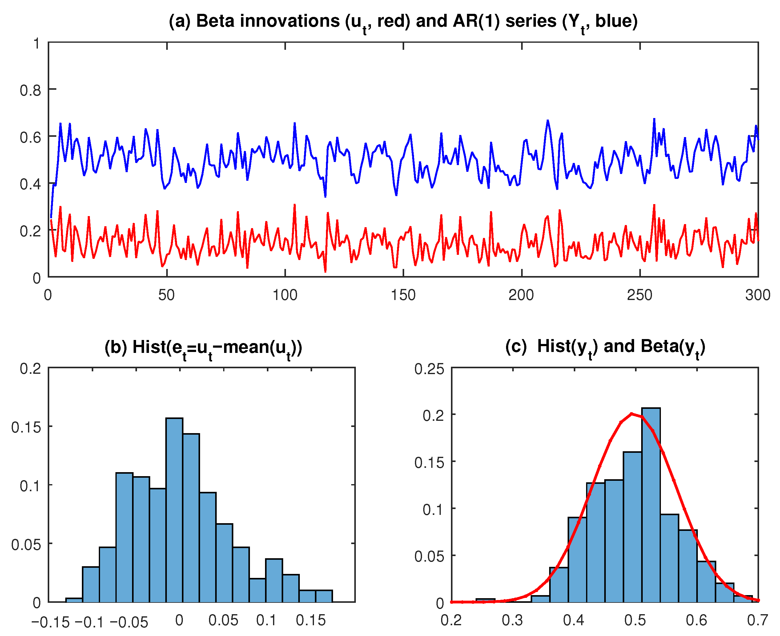
with starting values Y 0 = 0.25 and y 0 = 0. Figure 3 shows a realization of process (15a) with T = 300 ; the series Y t has a beta distribution in Figure 3c with estimated parameters α ^ y = 26.7 and β ^ y = 27.1. Instead, the process (15b) is nearly unstable, with a greater signal-to-noise ratio σ y / σ e .
Table 1 reports the basic statistics of fitting N = 500 realizations of the models (15a,b) with LS and ML estimators applied to the series Y t , Z t = ( Y t ) . The results show the better performance of the LS method in (15a); in particular, for the drift coefficient α 0 , which is affected by the logit transformation and cannot be converted into the original scale of (15a) using 1 ( α ˜ 0 ) . Instead, when only AR parameters are involved in (15b), the ML estimator is the best, with the hybrid close.

3. Applications to Real Data

3.1. US Monthly Unemployment Rate

In this section, we conduct an in-depth evaluation of the forecasting performance of linear and beta models using real data. The series in Figure 1 seems affected by various nonstationary components (in level, autocovariance, heteroskedasticity, etc.), but the most dangerous issue for model inference is the presence of a big jump in 2020. Sudden changes in Y t produce outliers in the residuals, which, in turn, make parameter estimates and forecasts biased and inefficient. A good method to contrast these effects is the introduction of pulse (dummy) or step variables as X t = 0 , 0 , 1 , 1 , 1 in correspondence with the anomalous residuals (see [18], Chapter 13). However, this solution is not applicable in forecasting, as the jumps are unpredictable and the effects of X t can be estimated only after their occurrence.
1. Model Identification.
To show the extent of the problem, we fit linear and beta AR(12) models to the whole series in Figure 1a and drop non-significant coefficients ϕ ^ k stepwise, as in Equation (5); surprisingly, both models reduce to AR(1)
Y t = 0.0017 ( 2.71 ) + 0.970 ( 94.7 ) Y t 1 + e t , σ ^ e = 0.0041 , H e = 0.447 [ 0.50 ] ,
Y t = 1 0.0686 ( 3.69 ) + 0.975 ( 145.7 ) Z t 1 + u t , δ ^ = 4652.8 ( 21.4 ) , H u = 1.048 [ 0.31 ] ,
where the values in parentheses are t-type statistics and δ is the precision parameter of the beta model. H e is Engle’s test for heteroskedasticity; the p-values in square brackets result in the hypothesis of homoskedastic residuals being accepted.
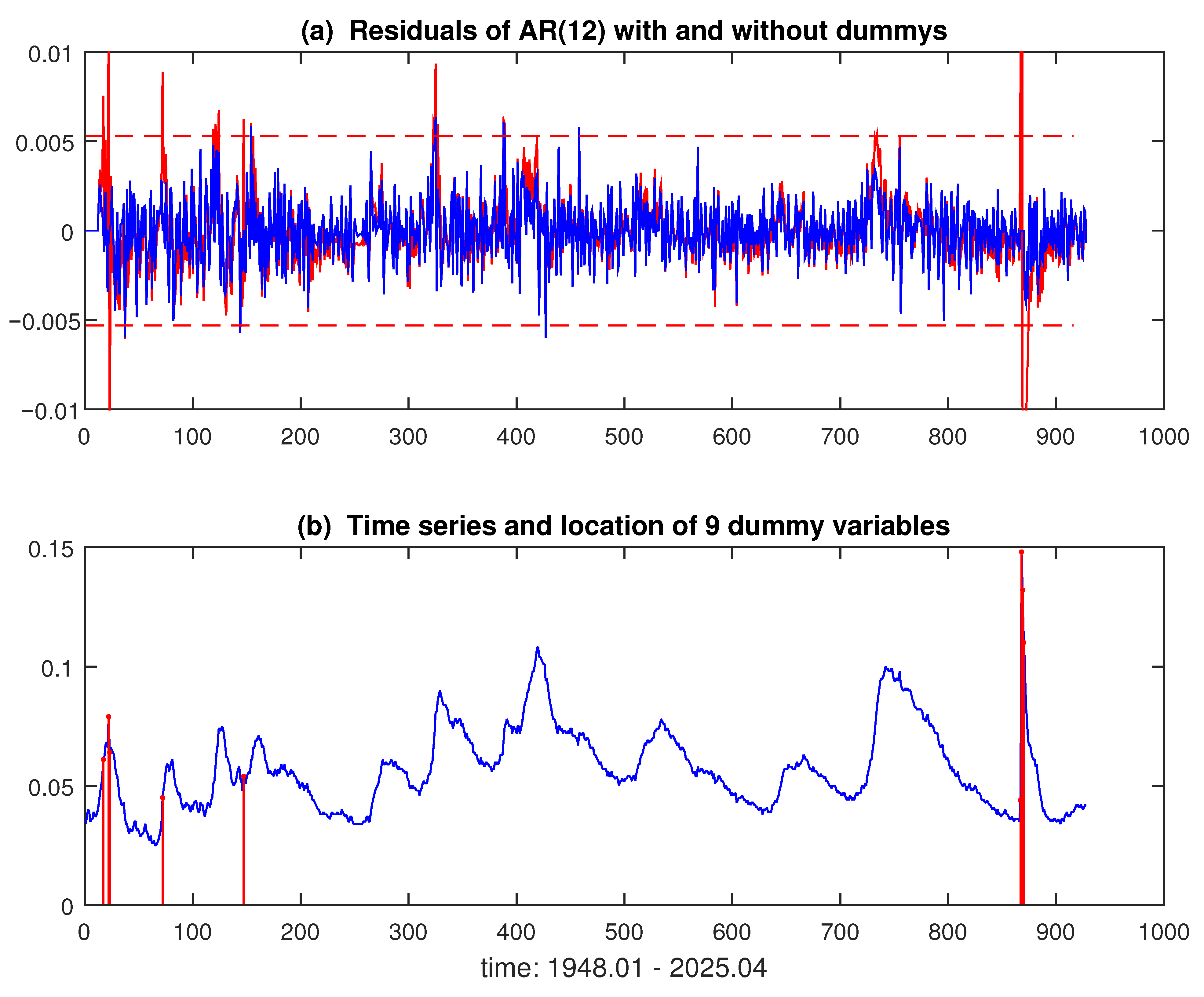
Now, the introduction of nine dummy variables, in correspondence with major outlying residuals (see [18], p. 482) increases the parametric complexity of Equation (16a,b), leading to subset AR(10) models. In general, dummy variables tend to self-feed (as dropping a major outlier often yields another minor one), and have uncertain effects on the model structure. Since sudden jumps are unpredictable, and we are interested in comparing the forecasting performance of the models, we will avoid using dummies and look for other solutions.
Figure 4 shows the cleaning effect of nine dummy variables on the residuals; since they are placed at the beginning and at the end of the series, we decide to restrict the analysis to the central part of Y t , namely from 1949.01 to 2019.12, a total of T = 852 observations. On this interval, the linear and beta AR models, identified with the stepwise method (5), retain the same structure:
Y t = 0.0008 ( 3.62 ) + 1.109 ( 83.6 ) Y t 1 0.124 ( 9.2 ) Y t 6 + e t , σ ^ e = 0.0018 , σ ˜ e = 0.0016 ,
Y t = 1 0.040 ( 3.57 ) + 1.101 ( 107.1 ) Z t 1 0.115 ( 11.2 ) Z t 6 + u t , δ ^ = 16455 ( 20.5 ) ,
where σ ˜ e is the robust, mean absolute deviation (MAD), estimate of the standard deviation, the fact that σ ^ e σ ˜ e in (17a) confirms the absence of outliers during the period 1949–2019. The subset nature of models (17) is highlighted by the peculiar term Y t 6 (non-seasonal); this lag is difficult to detect with classical methods (correlograms and information criteria) used for regular models, as those in [18].
2. Forecasting Evaluation.
Given the nonstationarity of the data, the design of the experiments for comparing the forecasts of the models (17) involve the rolling regression outlined in Equations (12)–(14); in practice:
(1)
The span H of the predictors (10) is set to one year: h = 1 , 2 12 ;
(2)
The out-of-sample forecasting period starts at t 0 + 1 = 517 (1991.01);
(3)
Models are estimated on t t 0 , with sample sizes n = 50 , 100 500 ;
(4)
At each t = t 0 + 1 T H , the parameters and forecasts are recomputed;
(5)
Prediction statistics are the mean absolute percentage errors (MAPE) (13c).
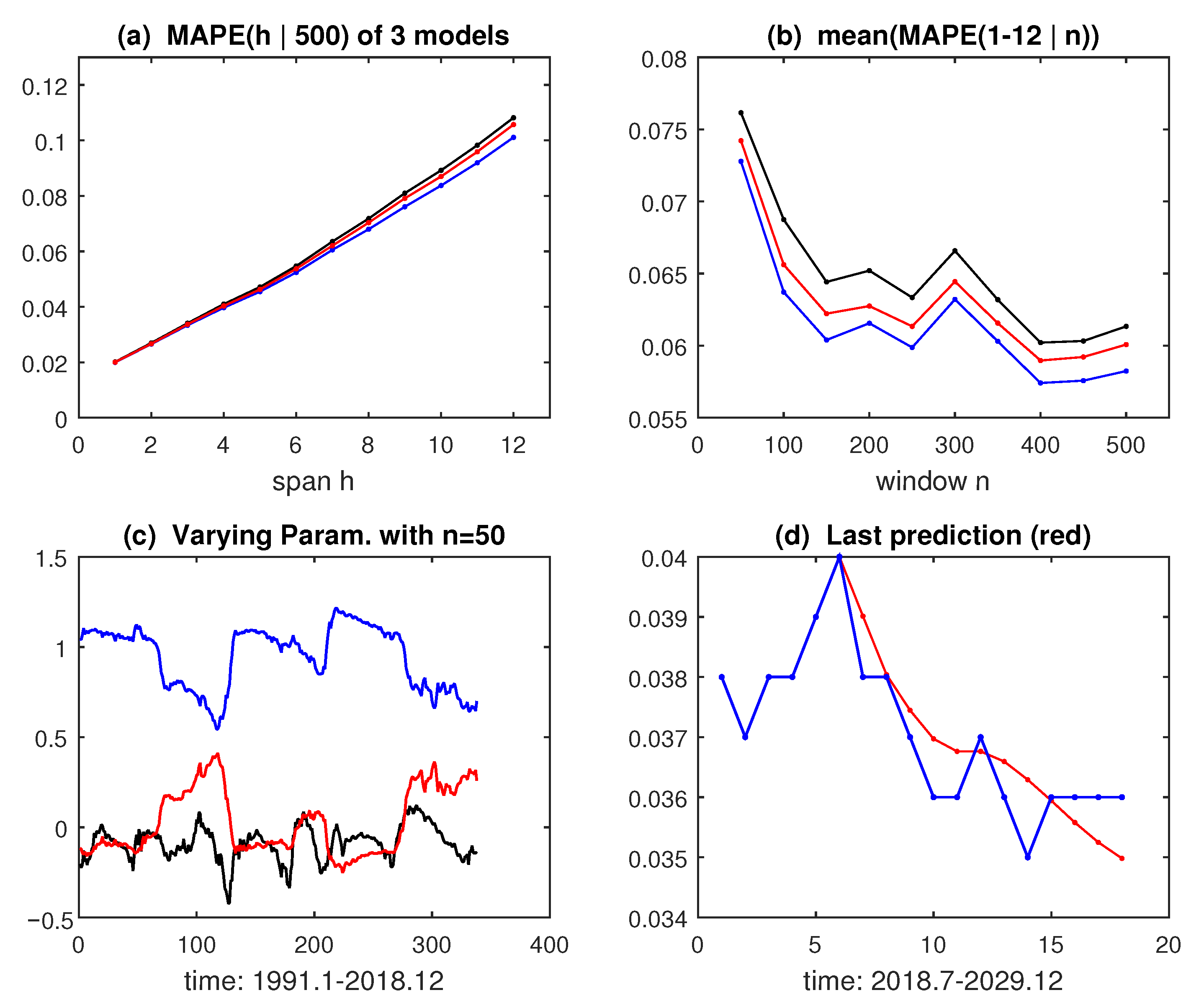
The results of this procedure are displayed in graphical form in Figure 5; Panel (a) shows that, with n = 500, the three models (linear, beta and hybrid) have a similar performance with a small predominance of the hybrid one (the linear modeling of the logit Z t = ( Y t ) ) . Panel (b) shows the effect of the estimation window n on the annual average of MAPE statistics; in this case, the difference among the three models seems greater, but the common best window is n = 400. Panel (c) shows the time-path of the parameters α 0 , ϕ 1 , ϕ 6 for n = 50 in the forecasting period, and Panel (d) shows the last forecast at T 12 (both for the hybrid model).
The main conclusion of Figure 5 is that the hybrid solution (linear AR modeling of the logit-transformed data, with inverse transformation in forecasting) is slightly better than the others. The distortion induced by the Jensen inequality does not appear, and the best window-width for the rolling regression is relatively large, i.e., n = 400, about 33 years.
3. Joint Selection of p,n.
Following Equation (14), we evaluate the joint effect of the model order p and sample size n on the MAPE(h) statistics of regular AR(p) models, in the same way as Figure 5b. The rationale of using all coefficients { ϕ k } 1 p is that some ϕ k t may locally be significant in the out-of-sample period t > t 0 and may be useful in forecasting; similarly, the selection of n should be based on prediction errors, rather than in-sample residuals. The results for H = 1, 12 are displayed in Figure 6 for the hybrid model; the optimal values during the period 1991–2019 are p ^ = 8, n ^ = 400. This means that parsimonious AR models ( p 3 ) are not suitable for both short- (h = 1) and long-range forecasts of the US unemployment series.

3.2. BR Hydroelectric Energy Storage

The second application deals with a dataset investigated with beta dynamic models by [13], but not compared with the corresponding linear models. The series regards the proportion of hydroelectric energy stored in South Brazil, i.e., the megawatts that can be generated from a stored volume of water, as a proportion of the total capacity. The monthly series covers the period 2000.07 to 2018.04 (a total of T = 214, see Figure 7a) and is provided by the Brazilian Electric Energy Agency [21]. The authors [13] compare several beta ARMA models in forecasting the last six values, including a beta-AR(3) estimated on the first t 0 = 150 observations. Table 2 confirms their parameter estimates in ([13], Table 9), except for standard errors, which indicate an AR(2) (consistent with the correlograms in ([13], Figure 1)).
The authors [13] show that their beta AR(3) outperforms the beta ARMA(2,1) in forecasting the last six data, as can be seen in ([13], Table 10); this may be due to the short prediction range of the MA components [18]. We now evaluate the in-depth forecasting performance of AR(2) models with the procedure (13), by setting t 0 = 151, p = 2, n = 50, 100, 150, h = 6; the results are reported in Figure 7.
We considered AR(2) models because our estimates of the coefficient ϕ 3 in Table 2 are not significant, and their MAPE statistics are smaller than those of the AR(3). Furthermore, we assessed that AR(3) predictions of the linear model go beyond the bound 1 at some points and need to be censored. Although the hydroelectric series is nearly stationary, the results of Figure 7 agree with those of Figure 5; in particular, there are not significant differences between the three models, and the best sample size n for the rolling estimations is not small.
Finally, to check nonstationarity, Figure 8 displays the rolling ML estimates of Equation (11) with n = 50 of the parameters of the beta AR(2) model. A certain time-variability is present, particularly in the precision parameter δ ^ t in Panel (b); notice also that the variances of u ^ t = ( Y t μ ^ t ) , obtained with the descriptive statistic s u 2 and the analytical formula σ ^ t 2 = μ ^ t ( 1 μ ^ t ) / ( 1 + δ ^ t ) , have the same pattern.

4. Conclusions

This paper has compared linear and beta autoregressive models in forecasting percentage time series in (0,1). Such series are often present in the real world, and in theory, should be treated with generalized linear models and maximum likelihood estimators. Instead, practitioners often fit them with classical linear models and ordinary least squares; the major risk is the bias of out-of-range forecasts and the inefficiency due to the heteroskedasticity in the presence of asymmetric distributions. On the other hand, the full beta modeling, by relying on the logit transformation of data, provides parameter estimates that are difficult to interpret, and the inverse transformation for obtaining forecasts in (0,1) may yield bias.
In the applications, we have seen that statistical differences, in fitting and forecasting between linear and beta AR models are not significant. This may mean that the bias of linear models (forecasts outside the range) and the bias induced by the inverse transformation (via the Jensen inequality) are similar. Now, the first bias can be easily detected (and corrected), and we checked that it is sporadically present only in the second application (where the series is concentrated near the upper border). For nonstationary time series, the best solution turned out to be the hybrid one (the linear modeling of logit-transformed data), because the use of logit transformation may mitigate the inefficiency due to heteroskedasticity. Instead, for stationary time series with strongly asymmetric distribution, the full beta modeling is preferable. Owing to the change of scale produced by the logit, a problem of interpretation of the coefficients of exogenous components remains.
The evaluation approach of this paper is based on MAPE statistics computed on long-range predictions and wide out-of-sample periods. This approach has been combined with the rolling estimation (also applied to the ML of beta models), leading to a predictive selection strategy of the model order p and the sample size n of the estimator; see Equation (14) and Figure 6. Notice that prediction errors e ^ t ( h ) are more challenging than the usual in-sample residuals and may be defined on multiple horizons h. The restriction of the analysis to pure AR models was motivated by their long-range forecasting ability and by their simple regression structure, which allows the direct application of complex statistical techniques.
Specifically, the maintenance of the linear structure (including the hybrid solution) is a necessary condition for extending the modeling toward adaptive methods, such as Kalman filters, M-type estimators, nonparametric smoothers, etc. [11]. These solutions are necessary in the presence of nonlinear dynamics, time-varying parameters, jumps in the series, and multiple outliers; instead, adaptive methods can hardly be implementable within the iterative ML framework (9) of the full beta approach. These are directions for further research, together with the comparison of the forecasts of nonlinear beta models [15,16] with those of the nonlinear models of econometrics (e.g., bilinear, threshold, state-space, ARCH, etc.).

Funding

This research received no external funding.

Data Availability Statement

Data and Software used in this research are available in the References [17,21,22,23], and their links.

Conflicts of Interest

The author declare no conflicts of interest.

Appendix A. Computational Aspects

This Appendix provides the computational details of the parameter estimator of the beta AR model. The Hessian matrix (9c) can be computed numerically with the finite difference method based on pairwise perturbation of its entries, namely
H i j ( δ ) = [ log L T δ 1 δ i + ε i δ j + ε j δ m log L T δ 1 δ i + ε i δ j δ m log L T δ 1 δ i δ j + ε j δ m + log L T δ 1 δ i δ j δ m ] 1 ε i ε j ,
where m is the length of δ and ε i = ϵ 3 ( 1 + | δ i | ) with ϵ set to the computer precision. This approach is followed by the optimization functions of the Matlab R2015a software we used; the computer code for estimating and forecasting a beta autoregressive model is based on the script of [22] and is placed in the repository [23]. Here, there is a synthesis for understanding the algorithms:
  •      function [bb, Zb, R2, yf] = ARbeta(y, p, h)
    % PURPOSE: ML estimation and forecast of an AR(p) model
    % for stationary data 0 < yt < 1 having a Beta distribution
    % INPUT: y = n*1 vector of time series data in (0,1)
    % p = 1,2 … order of the lags of the AR(p)
    % h = 1,2 … number of forecasts
    % OUTPUT: bb = ML estimates of parameters
    % Zb = T-type statistics of significance
    % R2 = pseudo R-squared index
    % yf = fitted and forecast values
    % USAGE: [bb, Zb, R2, yf] = ARbeta(y, 6, 12)
    n = length(y);
    yl = log(y./(1-y));
    X = zeros(n-p,p);
    for i = 1:p
    X(:,i) = yl(p-i+1:n-i);
    end
    X = [ones(n-p,1), X];
    bl = inv(X’*X)*(X’*yl(p+1:n));
    ylo = X*bl;
    muo= 1./(1+1./exp(ylo));
    so = sum((yl(p+1:n)-ylo).^2)/(n-2*p-1);
    pho = mean(1./(so*(muo.*(1-muo))))-1;
    bo = [ bl; pho ];
    options = optimset(’MaxFunEvals’,1230,’MaxIter’,1230);
    [bb,∼,∼,∼,∼,H]= fminunc(@(b) betalike(b, X, y(p+1:n)), bo, options);
    Vb = diag(pinv(H));
    Zb = bb./sqrt(abs(Vb));
    yl1 = X*bb(1:p+1);
    mu1 = 1./(1+1./exp(yl1));
    R2 = corr(yl1,yl(p+1:n))^2;
    ylf = [yl(1:p); yl1; zeros(h,1)];
    for t = n+1:n+h
    ylf(t) = bb(1)+ flip(bb(2:end-1))’*ylf(t-p:t-1);
    end
    yf = exp(ylf)./(1+exp(ylf));
    sf = std(y-yf(1:n));
    figure; subplot(211); plot(y,’-b’); hold on; plot(yf,’-r’)
    title(’(a) Original data Yt (blue), and beta AR fitted values (red)’)
    subplot(212); plot(yf(n-2*h:n+h),’.-r’); hold on; plot(y(n-2*h:n),’.-b’)
    plot(yf(n-2*h:n+h)+2*sf,’-k’); plot(yf(n-2*h:n+h)-2*sf,’-k’)
    title(’(b) Original data Yt (blue), and beta AR forecasts (red)’)
    xlabel(’Time: T-2h:T+h’)
    % Likelihood function ----------------------------------------------
    function ll = betalike(b, X, y)
    yo = X*b(1:end-1);
    mu = exp(yo)./(1+exp(yo));
    phi = b(end);
    ll = -sum(gammaln(phi) - gammaln(mu*phi) - gammaln((1-mu)*phi) + …(mu*phi-1).*log(y) + ((1-mu)*phi-1).*log(1- y) );

References

  1. Hurata, A.D. Predicting the unemployment rate using autoregressive integrated moving average. Cogent Bus. Manag. 2024, 11, 2293305. [Google Scholar] [CrossRef]
  2. Coskun, C.; Oktay, Z.; Birecikli, B.; Bamya, S. Energy and economic analysis of a hydroelectric power plant. Eur. J. Eng. Technol. Res. 2023, 8, 43–47. [Google Scholar] [CrossRef]
  3. Haile, G.G.; Tang, Q.; Hosseini-Moghari, S.-M.; Liu, X.; Gebremicael, T.G.; Leng, G.; Kebede, A.; Xu, X.; Yun, X. Projected impacts of climate change on drought patterns over East Africa. Earth Future 2020, 8, e2020EF001502. [Google Scholar] [CrossRef]
  4. Rosenfeld, R.; Berg, M. Forecasting future crime rates. J. Contemp. Crim. Justice 2024, 40, 218–231. [Google Scholar] [CrossRef]
  5. Grillenzoni, C. Robust time-series analysis of the effects of environmental factors on the COVID-19 pandemic in the area of Milan (Italy) in the years 2020–2021. Hyg. Environ. Health Adv. 2022, 4, 100026. [Google Scholar] [CrossRef] [PubMed]
  6. East, S.D.; Zahed, M. Forecasting U.S. unemployment rates using ARIMA: A time series analysis from 1948 to 2019. In Proceedings of the SESUG Conference, Washinghton, DC, USA, 22–24 September 2024. [Google Scholar]
  7. Zhang, D. Forecasting USA unemployment rate based on ARIMA model. Adv. Econ. Manag. Political Sci. 2023, 49, 67–76. [Google Scholar]
  8. Saraf, N.; Bemporad, A. A bounded-variable least-squares solver based on stable QR updates. IEEE Trans. Autom. Control 2020, 65, 1242–1247. [Google Scholar] [CrossRef]
  9. Kieschnick, R.; McCullough, B.D. Regression analysis of variates observed on (0, 1): Percentages, proportions and fractions. Stat. Model. 2003, 3, 193–213. [Google Scholar] [CrossRef]
  10. Qasim, M.; Mansson, K.; Kibria, B.M.G. On some beta ridge regression estimators: Methods, simulation and application. J. Stat. Comput. Simul. 2021, 91, 1699–1712. [Google Scholar] [CrossRef]
  11. Grillenzoni, C. Forecasting unstable and nonstationary time series. Int. J. Forecast. 1998, 14, 469–482. [Google Scholar] [CrossRef]
  12. Rocha, A.V.; Cribari-Neto, F. Beta autoregressive moving average models. Test 2009, 18, 529–545. [Google Scholar] [CrossRef]
  13. Cribari-Neto, F.; Scher, V.; Bayes, F. Beta ARMA selection with application to modeling and forecasting stored hydroelectric energy. Int. J. Forecast. 2023, 39, 98–109. [Google Scholar] [CrossRef]
  14. Zeileis, A. Why Use the Logit Link in Beta Regression? 2018. Available online: https://stats.stackexchange.com/questions/337115/ (accessed on 31 May 2025).
  15. Scher, V.T.; Cribari-Neto, F.; Bayer, F.M. Generalized ARMA model for double bounded time series forecasting. Int. J. Forecast. 2024, 40, 721–734. [Google Scholar] [CrossRef]
  16. Pierrot, A.; Pinson, P. On tracking varying bounds when forecasting bounded time series. Technometrics 2024, 66, 651–661. [Google Scholar] [CrossRef]
  17. US Bureau of Labor Statistics Civilian Unemployment Rate. 2025. Available online: https://www.bls.gov/charts/employment-situation/civilian-unemployment-rate.htm (accessed on 30 April 2025).
  18. Box, G.E.P.; Jenkins, G.M.; Reinsel, G.C.; Ljung, G.M. Time Series Analysis: Forecasting and Control, 5th ed.; Wiley: New York, NY, USA, 2015. [Google Scholar]
  19. Lee, J. Asymptotic property of least squares estimators for explosive autoregressive models with a drift. Jour. Econ. Theory Econ. 2021, 32, 1–12. [Google Scholar]
  20. King, G.; Roberts, M.E. How robust standard errors expose methodological problems they do not fix, and What to do about it. Political Anal. 2015, 23, 159–179. [Google Scholar] [CrossRef]
  21. Operador Nacional do Sistema Elétrico Energia Armazenada. 2020. Available online: http://www.ons.org.br/historico/energia_armazenada.aspx (accessed on 30 April 2025).
  22. De Goeij, W.-J. Beta Regression, Matlab Code. 2009. Available online: https://it.mathworks.com/matlabcentral/fileexchange/24994 (accessed on 31 July 2025).
  23. Grillenzoni, C. Beta Autoregressive Models for Forecasting Percentage Series. 2025. Available online: https://it.mathworks.com/matlabcentral/fileexchange/181667 (accessed on 31 August 2025).
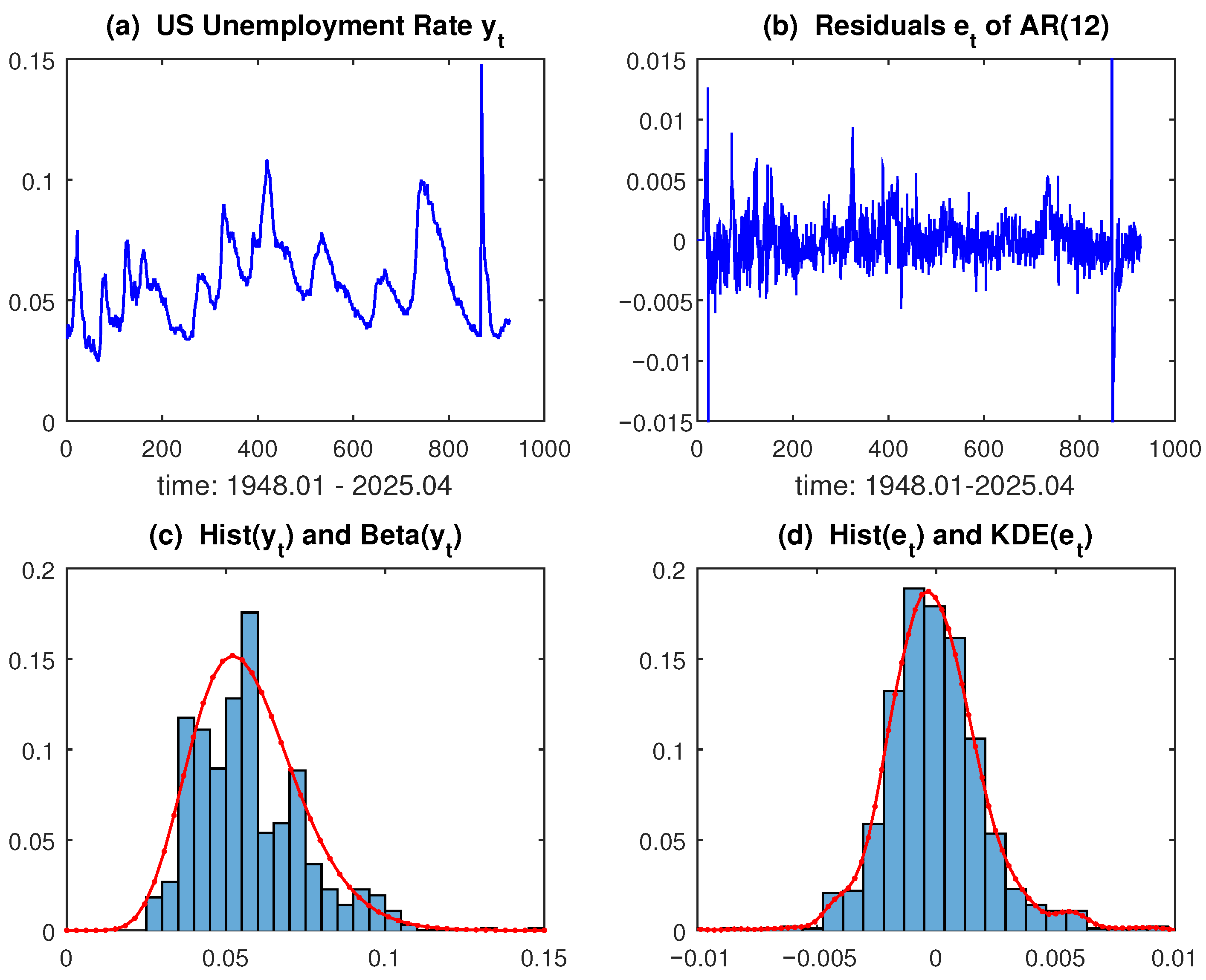
Figure 1. Preliminary data analysis: (a) US monthly unemployment rate Y t from 1948.01 to 2025.04; (b) Residuals e ^ t obtained by fitting Y t with an AR(12) model; (c) Histogram and Beta (11,183) density of Y t ; (d) Histogram and Kernel density (KD) of e ^ t .
Forecasting 07 00057 g001
Figure 2. Representation of the sequential procedure (13): moving sample (blue); prediction period (red); regression function (green).
Forecasting 07 00057 g002
Figure 3. Display of a simulation of model (15a): (a) Series Y t (blue) and beta innovations u t (red); (b) Histogram of e t = ( u t u ¯ t ) ; and (c) Histogram of Y t and its beta density f ( Y ) .
Forecasting 07 00057 g003
Figure 4. Effects of dummy variables on a linear AR(12) model: (a) Residuals with (blue) and without (red) the dummies; (b) Location of the dummies in the series.
Forecasting 07 00057 g004
Figure 5. Results of the procedure (13) on the models (17): linear (black), beta (red), hybrid (blue): (a) MAPE( h = 1 12 ) statistics during the period 1991–2019, with n = 500; (b) Effects of the size n on the average 12 1 h MAPE(h); (c) Time-varying parameters of the hybrid model with n = 50, in the forecasting period; and (d) Last prediction Y ^ T 12 + h (red).
Forecasting 07 00057 g005
Figure 6. Effect of the sample size n and model order p on the MAPE(h) statistics in the period 1991.01–2019.12: (a) MAPE(h = 1); (b) average(MAPE(1–12)).
Forecasting 07 00057 g006
Figure 7. Results of the procedure (13) applied to AR(2) models: linear (black), beta (red), hybrid (blue); (a) Graph of the Brazilian energy data; (b) Beta density estimate with α ^ = 3.10 and β ^ = 1.29; (c) MAPE( h = 1 6 ) statistics during the period 2013.01–2018.04, with sample n = 150; (d) Effects of the size n on 6 1 h MAPE( h | n ).
Forecasting 07 00057 g007
Figure 8. Rolling ML estimates with n = 50 of the beta AR(2) model applied to data in Figure 7: (a) Structural parameters: α ^ 0 t (black), ϕ ^ 1 t (red), ϕ ^ 2 t (blue); and (b) Dispersion parameters: δ ^ t /500 (black), descriptive σ ^ t 2 (red), analytical σ ^ t 2 (blue).
Forecasting 07 00057 g008
Table 1. Performance of ML (9) and LS (3) estimators applied to the models (15a,b); Bias, RMSE, mean p-value of the Jarque–Bera normality test are computed over 500 replications of length T = 300.
(15a) α 0 ϕ 1
ModelMethodBiasRMSEN-testBiasRMSEN-test
Linear (1a)LS (3)0.00250.02550.133−0.00500.05110.1350
Hybrid (7b)LS (3)−0.24940.24950.001−0.00740.05120.1307
Beta (7c)ML (9)−0.24940.24950.001−0.01410.05210.1546
(15b) ϕ 1 ϕ 2
ModelMethodBiasRMSEN-testBiasRMSEN-test
Linear (1a)LS (3)0.04680.06690.02840.04870.06870.0326
Hybrid (7b)LS (3)−0.00610.04950.0010−0.00090.04870.0010
Beta (7c)ML (9)−0.01010.04930.01020.00120.04720.0936
Table 2. Estimates of AR(3) models on the first n = 150 data of Figure 7a; standard errors are in parentheses and p-values in square brackets. H e is the Engle’s homoskedastic test.
ModelMethod α 0 ϕ 1 ϕ 2 ϕ 3 δ , σ e R 2 H e
Beta([13], Table 9). 0.949 ( 0.033 ) 0.338 ( 0.051 ) 0.087 ( 0.042 ) ...
BetaML (9) 0.211 ( 0.067 ) 0.967 ( 0.079 ) 0.372 ( 0.103 ) 0.118 ( 0.070 ) 14.11 ( 1.63 ) 0.654 ( pseudo ) 0.534 [ 0.465 ]
LinearLS (3) 0.156 ( 0.037 ) 1.146 ( 0.080 ) 0.439 ( 0.116 ) 0.068 ( 0.081 ) 0.1040.722 0.429 [ 0.512 ]
Disclaimer/Publisher’s Note: The statements, opinions and data contained in all publications are solely those of the individual author(s) and contributor(s) and not of MDPI and/or the editor(s). MDPI and/or the editor(s) disclaim responsibility for any injury to people or property resulting from any ideas, methods, instructions or products referred to in the content.