Abstract
This research introduces a system designed to predict three-dimensional airspace occupancy over Colombia using historical Automatic Dependent Surveillance-Broadcast (ADS-B) data and machine learning techniques. The goal is to support proactive air traffic management by estimating future aircraft positions—specifically their latitude, longitude, and flight level. To achieve this, four predictive models were developed and tested: K-Nearest Neighbors (KNN), Random Forest, Extreme Gradient Boosting (XGBoost), and Long Short-Term Memory (LSTM). Among them, the LSTM model delivered the most accurate results, with a Mean Absolute Error (MAE) of 312.59, a Root Mean Squared Error (RMSE) of 1187.43, and a coefficient of determination (R2) of 0.7523. Compared to the baseline models (KNN, Random Forest, XGBoost), these values represent an improvement of approximately 91% in MAE, 83% in RMSE, and an eighteen-fold increase in R2, demonstrating the substantial advantage of the LSTM approach. These metrics indicate a significant improvement over the other models, particularly in capturing temporal patterns and adjusting to evolving traffic conditions. The strength of the LSTM approach lies in its ability to model sequential data and adapt to dynamic environments—making it especially suitable for supporting future Trajectory-Based Operations (TBO). The results confirm that predicting airspace occupancy in three dimensions using historical data are not only possible but can yield reliable and actionable insights. Looking ahead, the integration of hybrid neural network architectures and their deployment in real-time systems offer promising directions to enhance both accuracy and operational value.
1. Introduction
Global aviation has evolved rapidly in recent decades, establishing itself as a strategic pillar for mobility and economic integration on a worldwide scale. According to the International Civil Aviation Organization (ICAO), demand for air transportation services is expected to grow at an annual rate of 4.3% over the next 20 years, with more than 100,000 commercial flights already operating daily [1]. This sustained growth has placed increasing pressure on air navigation systems, prompting the need for more efficient, safer, and environmentally sustainable airspace management strategies. In response to these challenges, international initiatives such as the Global Air Navigation Plan (GANP) have proposed a comprehensive redesign of air traffic management, introducing concepts like Trajectory-Based Operations (TBO) and process digitalization [2,3].
One of the most pressing challenges in air traffic management today is the ability to accurately predict three-dimensional (3D) airspace occupancy, simultaneously accounting for latitude, longitude, and altitude. This predictive capacity is crucial for anticipating traffic density in strategic sectors, minimizing the risk of conflicts, enabling more efficient routing in real time, and ultimately contributing to reduced fuel consumption. The complexity of this task is magnified in countries like Colombia, where the airspace is shaped by highly diverse geographic and operational conditions.
The Colombian national territory spans three major mountain ranges, vast jungle regions, expansive plains, and dual coastlines on the Caribbean and Pacific. This geographic variety is matched by a broad and unevenly distributed network of airports, including both controlled and uncontrolled facilities. As air traffic continues to increase, driven by the steady growth of tourism and commercial activity, certain air corridors have begun to experience significant congestion, making the need for accurate 3D forecasting more urgent than ever [4].
Currently, flight route planning in Colombia relies on standardized procedures published in the Aeronautical Information Publication (AIP). These procedures require aircraft to follow predefined routes established through designated waypoints, in accordance with the General Flight Rules set forth in the Colombian Aeronautical Regulations, specifically Chapter 91 (RAC 91) [5].
Although systems such as Area Navigation (RNAV) and Required Navigation Performance (RNP) have improved navigational accuracy, they do not dynamically incorporate weather data, traffic conditions, or operational performance parameters. As a result, inefficiencies, unexpected route deviations, and increased fuel consumption often occur [6,7]. Unlike regions such as Europe and the United States, where strategies like Free Route Airspace (FRA) and advanced planning platforms have been implemented [8,9,10], Colombia has not yet adopted a predictive approach based on Artificial Intelligence (AI).
Figure 1 illustrates the European airspace, where the FRA concept is already in use. This operational concept allows aircraft to plan routes freely between a defined enter point and exits points within a designed airspace, rather than being contrasted to fixed airways. By enabling more direct trajectories, this approach contributes to more efficient trajectories, and improved airspace management, FRA contributes to improved efficiency, increased airspace capacity, and reduced environmental impact through lower fuel consumption.
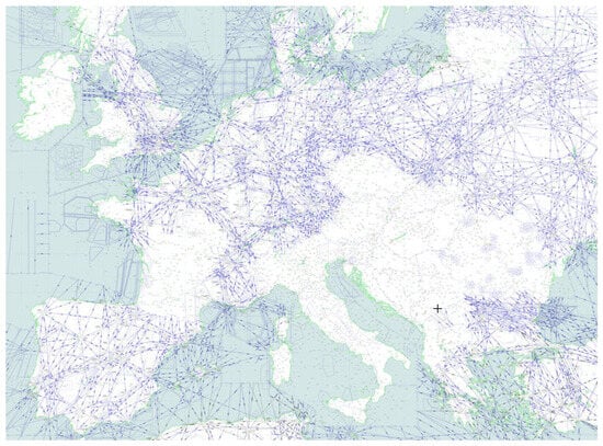
Figure 1.
Illustration of the FRA concept in Europe. The blue lines represent predetermined routes, while the blank areas indicate the countries where the FRA concept has been implemented [11].
In this context, scientific advancements in AI and Machine Learning (ML) have demonstrated significant potential to transform air route planning. Various studies have employed deep learning algorithms such as Convolutional Neural Networks (CNNs), Long Short-Term Memory (LSTM) networks, hybrid CNN-LSTM models, and autoencoders to predict fourth-dimension (4D) trajectories using ADS-B data and weather conditions, achieving higher levels of accuracy compared to traditional methods [12,13]. Recent research has also integrated Artificial Neural Networks (ANNs), Hidden Markov Models (HMMs), and stochastic optimization strategies to capture atmospheric and operational variability, thereby improving planning in real-world scenarios [14,15].
Furthermore, systems have been developed that incorporate aircraft tactical intent, reinforcement learning techniques (e.g., Light Gradient Boosting Machine [LGBM], Multilayer Perceptron [MLP], Support Vector Machines [SVMs]), and the detection of significant events through time series analysis. These systems have successfully addressed both trajectory prediction and risk assessment, particularly in terminal environments and complex operations [16,17,18]. In specific applications, these models have proven capable of predicting aircraft climb and descent phases, trajectory losses, landing speeds, and even risk events in aircraft carrier operations, using algorithms such as XGBoost, Bidirectional LSTM (BLSTM), and Extreme Learning Machines (ELMs) combined with Particle Swarm Optimization (PSO) [19,20,21,22,23,24].
In the airport domain, progress has also been made in the application of data mining techniques for the prediction of delays, detection of abnormal runway occupancy, and improvement of surface movement management using CNN models and hierarchical clustering [25,26,27,28]. These applications demonstrate the ability of machine learning models to provide high-fidelity predictions that support decision-making in complex and dynamic operational environments.
As can be seen, in other parts of the world different algorithms are already being developed to predict aspects such as flight delays, abnormal runway occupancy, and trajectory deviations. These algorithms support air traffic controllers in decision-making by reducing workload and enhancing situational awareness. In addition, they contribute to greater operational efficiency, improved safety margins, and more sustainable airspace management.
As previously mentioned, air traffic in Colombia is expected to grow, which in turn poses several challenges such as flight delays, airspace congestion, and an increased workload for controllers. Addressing these issues requires innovative tools that enhance automation and promote the adoption of novel operational concepts and technologies. In this context, airspace occupancy prediction becomes a key enabler for optimizing air traffic operations, as it allows for the identification of occupied airspace and provides controllers with more comprehensive situational awareness. This, in turn, enables them to anticipate potential conflicts and determine more efficient routes, thereby improving airspace utilization and reducing fuel consumption.
This not only results in reduced fuel consumption and shorter trajectories but also highlights the value of knowing future airspace occupancy. Such information enables airport authorities and airline operators to make proactive decisions, optimizing flight scheduling as all stakeholders gain awareness of future traffic distribution. By ensuring better coordination between flight schedules, airspace capacity, and airport infrastructure, several advantages can be achieved for airlines, including increased customer satisfaction and lower operational costs through optimized routes.
Despite these advantages, Colombia has not yet adopted a system that incorporates predictive technologies to optimize its air routes. Airspace planning continues to follow a reactive approach, heavily reliant on commercial software and lacking the ability to forecast future operational scenarios. This shortfall not only leads to higher operational costs and increased emissions but also poses risks to the safety and efficiency of the country’s air navigation system.
To address this gap, the core objective of the project was to develop a predictive model capable of reliably estimating future aircraft positions within Colombian airspace. This 3D forecasting capability is intended to support both tactical and strategic decision-making processes, enhancing sector allocation and conflict management while contributing to a more efficient and responsive air traffic system. Beyond the Colombian context, the proposed approach also provides evidence of how machine learning techniques based on ADS-B data can be applied to complex and diverse airspaces, offering valuable insights for the global advancement of predictive air traffic management.
The fact that these types of models are not yet being developed in Colombia allows this research to serve as a foundation for future studies, not only at the national level but also regionally in South America, where efforts to implement predictive approaches in air traffic management remain scarce. In this sense, the contribution of the study lies in demonstrating the applicability of well-known models to a novel context, providing empirical evidence and methodological guidance for advancing predictive airspace management in regions where this field is still largely unexplored.
2. Materials and Methods
This research aimed to develop and evaluate an artificial intelligence model capable of predicting 3D airspace occupancy, specifically, aircraft positions expressed in latitude, longitude, and altitude, by analyzing historical flight trajectory data. The study relied on records obtained from ADS-B systems, which offer high-resolution data on aircraft movements and altitudes with near real-time precision. The analysis focused on flights within Colombian airspace, covering a wide range of geographic regions, altitude levels, and time periods. This comprehensive approach allowed for the identification of traffic patterns under varying operational conditions. Based on this historical dataset, several prediction models were constructed to estimate the spatial distribution of aircraft within specific future time intervals, aiming to improve situational awareness and support more efficient airspace management.
The methodology adopted in this study brought together key elements from two widely recognized frameworks: the Cross-Industry Standard Process for Data Mining (CRISP-DM) and Design Science Research (DSR). By combining these approaches, the research process was structured in a systematic and iterative way, ensuring both analytical rigor and practical relevance. The methodologies are described below:
- The CRISP-DM methodology guided the phases of understanding the operational context, exploring and preprocessing the ADS-B data, constructing predictive models, and evaluating the results obtained [6,29];
- Complementarily, the DSR approach allowed the predictive model to be conceived as a technological artifact, validated based on its usefulness for anticipating high-occupancy zones and its accuracy in predicting future positions within the three-dimensional airspace [30].
This integration provided a clear pathway for addressing a real-world challenge within the aviation sector, as illustrated in Figure 2. By combining these two methodologies, the research began with the identification and understanding of the problem, which guided the acquisition of the ADS-B data required for model training. Following the CRISP-DM framework, the dataset was explored, preprocessed, and validated to ensure its quality before proceeding to the modeling phase. The predictive models were then trained and evaluated using appropriate performance metrics. Complementarily, the DSR approach framed the predictive model as a technological artifact, whose value was assessed not only in terms of accuracy but also by its usefulness in anticipating high-occupancy zones and predicting future aircraft positions within the three-dimensional airspace.
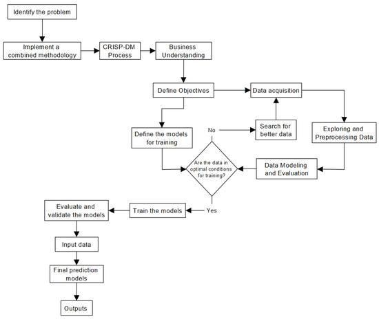
Figure 2.
Phases of the Combined CRISP-DM and DSR Methodology.
2.1. Problem and Objetives
Efficient management of airspace depends on the ability to anticipate how air traffic will be distributed across three dimensions. In Colombia, however, there is still a noticeable gap in both technological capacity and operational strategy when it comes to this kind of forecasting. Flight planning continues to rely on conventional procedures that lack advanced predictive tools, which limits the capacity to foresee 3D airspace occupancy defined by latitude, longitude, and altitude, and to proactively respond to high-density traffic or emerging conflict scenarios. This gap has a direct impact on operational efficiency, increases fuel consumption and flight times, and ultimately affects the sustainability of the entire air navigation system.
In light of this situation, the need emerged to design a predictive system capable of estimating airspace occupancy in Colombia using historical flight data, supported AI and ML techniques. Unlike other methods that depend on external variables such as weather or aircraft performance, this approach focuses exclusively on patterns derived from real-world flight trajectories recorded through ADS-B systems. This design choice ensures that the model remains both scalable and applicable to real operational environments.
As part of this first development phase, the project also identified key operational stakeholders such as airlines, air traffic controllers, and Air Navigation Service Providers (ANSP), whose roles, needs, and constraints were taken into account during the system’s design. Additionally, the initiative was aligned with the strategic objectives outlined by the ICAO in its GANP and grounded in the principles of TBO, which emphasize the importance of predictable, high-precision trajectories as the foundation for safe and efficient air traffic management.
2.2. Data Acquisition
The database used in this study was constructed using historical surveillance records collected through the ADS-B system, which allows aircraft to periodically transmit data on their position, speed, altitude, and other key parameters via radio frequency signals. Unlike traditional radar systems, ADS-B does not depend on active interrogation from ground stations. This enables more continuous, accurate, and cost-efficient monitoring, making it one of the core technologies currently supporting modern air traffic management.
The system works by having aircraft equipped with specialized transponders transmit navigation data based on inputs from Global Navigation Satellite Systems (GNSS). These broadcasts can be received by ground-based or satellite receivers, providing near real-time tracking of each aircraft’s trajectory. The resulting dataset includes geographic coordinates such as latitude and longitude, reported altitude, ground speed, heading, flight identification, aircraft model, and airline code, among other relevant attributes [31].
The data used in this study were sourced from Flightradar24, a globally recognized platform that operates an extensive network of ADS-B receivers and offers access to historical flight information. Flightradar24 has the infrastructure to collect millions of messages per second from aircraft in flight, making it a reliable and comprehensive source for air traffic analysis. Its database provides structured access to flight data categorized by date, flight type, origin and destination, and a range of technical and operational attributes.
For the purposes of this research, flight data from the year 2024 were downloaded and organized, covering both commercial and non-commercial flights within Colombian airspace. From this dataset, a representative subset was selected to ensure adequate geographic and operational diversity. ADS-B provides a wide range of variables, including ground speed at a given coordinate, departure and destination airports, aircraft identification, flight callsign, heading, and precision measures of the transmitted data. However, many of these variables were irrelevant to the objectives of this study. Therefore, only the variables directly related to the prediction task were retained. Specifically, the subset included the columns corresponding to date and time, longitude, latitude, and altitude; variables described in Table 1.

Table 1.
Description of dataset variables.
2.3. Data Processing
Data processing played a fundamental role in the development of the 3D airspace occupancy prediction system, as it allowed for the transformation and optimization of dataset variables prior to their use in machine learning models. The process was carried out in four key phases: cyclical encoding of temporal variables, feature scaling to standardize data ranges, dimensionality reduction to simplify the input space, and dataset splitting to enable effective training and evaluation of the predictive models.
2.3.1. Cyclical Encoding
One of the most important features of the dataset was the presence of temporal variables with a periodic nature, such as day of the week, hour of the day, and minute. Representing these variables linearly (e.g., using integer values from 0 to 6 for days of the week or 0 to 23 for hours) can lead to errors in machine learning, as their circular structure is not respected. For example, from a linear perspective, 11:00 p.m. and 12:00 a.m. may appear far apart, when in reality they are consecutive points in time [32].
To address this issue, a cyclical encoding method using sine and cosine trigonometric functions was applied. This technique transforms periodic variables into two new dimensions that represent their position on a unit circle, ensuring that sequential values remain close in the transformed space. For a variable such as the hour of the day, the applied transformations were:
In Equations (1) and (2), the variable hour represents the hour of the day, expressed as an integer between 0 and 23. The constant 24 corresponds to the total number of hours in a complete daily cycle, normalizing the variable to a fraction of the day. The factor 2π transforms this fraction into an angular value in radians, mapping the time onto the unit circle. Finally, the sine and cosine functions project this angle onto the vertical and horizontal axes, respectively, generating two complementary features (hour_sin and hour_cos) that jointly encode the cyclical behavior of time.
This procedure was repeated for other cyclical variables, such as minute and day of the week, allowing for the preservation of temporal continuity in the data and enhancing the model’s learning performance.
2.3.2. Feature Scaling
To normalize the magnitude of the numerical variables and facilitate the model training process, the MinMaxScaler method was used [33]. This technique adjusts all values of each feature to a range between [0, 1] using the following formula:
where represents the original values, is the minimum value of the feature, and is the maximum. This step is essential to ensure that all variables contribute equally to the learning process and to prevent features with larger scales from dominating model training.
2.3.3. Dimensionality Reduction with Principal Component Analysis
Principal Component Analysis (PCA) was selected as the dimensionality reduction technique in this study due to its simplicity, interpretability, and proven effectiveness in capturing variance while reducing input dimensionality. Unlike methods such as t-SNE, which are primarily designed for low-dimensional visualization, or autoencoders, which require additional training and hyperparameter tuning, PCA provides a deterministic and unsupervised transformation that yields orthogonal components ranked by explained variance. This makes it a practical choice in forecasting tasks where reducing redundancy and mitigating multicollinearity can improve model stability. Moreover, PCA is computationally efficient and introduces minimal design complexity, as the main decision lies in selecting the number of retained components. While PCA does not guarantee that the most predictive features are preserved, its balance of robustness, efficiency, and interpretability made it a suitable approach for this study’s time-encoded input features [34].
To reduce model complexity and eliminate potential redundancies, PCA was applied to the input variables. The technique transforms the original set of potentially correlated features into a new set of orthogonal variables, known as principal components, which retain most of the variance from the dataset. In this study, six principal components were selected, enabling dimensionality reduction without significant loss of critical information. This reduced representation facilitated more efficient data processing and contributed to preventing model overfitting during training [34].
2.3.4. Dataset Splitting
The dataset was partitioned into 80% for training and 20% for testing, a proportion widely documented in the literature for its effectiveness in balancing the volume of data allocated to model learning and independent validation [35]. To ensure the re-producibility of results and facilitate comparability across algorithms, a single random seed was fixed during the partitioning process for all models. The use of a fixed seed guarantees that the training and testing subsets remain consistent across runs, ensuring that observed differences in performance can be attributed solely to the predictive capacity of the models rather than to variations in the input data.
This practice aligns with established standards for reproducible experimentation, as emphasized in the methodological literature on machine learning [36]. Furthermore, the partitioning procedure was designed to preserve both temporal variability (days, hours, and years) and spatial variability (different geographic regions within Colombian airspace). This pre-caution was taken to avoid biases that might arise if subsets were concentrated within a single period or region, which could lead to overly optimistic estimates of prediction error. The importance of maintaining these structures during data splitting and cross-validation procedures has been highlighted in studies addressing time series and spatial data in complex prediction problems [35].
2.4. Model Training
The prediction task was formulated under a one-step ahead (point forecast) approach, meaning that each model estimates the future position of the aircraft (latitude, longitude, and flight level) at a specific instant in time, corresponding to a defined day, hour, and year. No multi-step iterative forecasts were generated, nor was the prediction extended to multiple future periods. The methodological decision to adopt a one-step ahead framework rests on two main considerations.
First, this approach generally provides greater stability in the results by avoiding the error accumulation characteristic of multi-step predictions. As highlighted in the time series and the air traffic modeling literature, error propagation tends to distort results over extended horizons. For instance, Ming et al. [37] demonstrates that in passenger traffic time series, one-step ahead forecasting allows a focus on immediate pointwise variations, thereby reducing distortions that become amplified when multiple steps are projected.
Second, in operational contexts where anticipation of events is required for a concrete future instant (e.g., a specific hour of a particular day), point forecasting is more practical and reliable. Additionally, to ensure applicability in real-world scenarios and prevent inadvertent use of future information during training, the one-step ahead framework ties each prediction to a fixed temporal reference: the model receives as input all available data up to that day, hour, and year, and produces the forecast precisely for that subsequent moment. This design ensures that the evaluation reflects real operational conditions, where future data beyond the prediction instant are never available [37].
At this stage, various AI algorithms were integrated and executed with the goal of modeling and predicting three-dimensional air traffic density (latitude, longitude, and altitude) within Colombian airspace. To achieve this, multiple supervised learning models were trained and evaluated to analyze large volumes of historical data in order to generate accurate predictions of future airspace occupancy. The prediction was focused on user-defined time windows, enabling the identification of critical congestion points and the planning of optimal flight routes.
The variables used for model training included latitude, longitude, and timestamp, which allowed for the capture of both spatial components and the temporal behavior of air traffic. These variables were selected due to their operational relevance and their availability within the historical records obtained through ADS-B systems. Once the model was trained, users could input a specific date and time, and the system would generate a prediction of the expected airspace occupancy for that time window, highlighting the regions with the highest traffic density in three dimensions.
The four main machine learning approaches selected for this study were KNN, Random Forest, XGBoost, and LSTM networks each selected for its ability to model different aspects of air traffic dynamics.
KNN was included as a simple yet effective baseline method for spatial approximation, exploiting local similarities between trajectories without requiring extensive training. Random Forest was selected as a robust ensemble technique capable of capturing nonlinear relationships and reducing variance through bagging, thus providing stable predictions even in noisy datasets. XGBoost, a state-of-the-art gradient boosting algorithm, was incorporated for its proven ability to handle large-scale, heterogeneous data and to improve accuracy by sequentially correcting residual errors.
Finally, LSTM networks were chosen as the most advanced model for this context, given their ability to capture sequential dependencies and long-term temporal patterns in time-series data such as flight trajectories. This makes LSTM particularly suitable for forecasting future airspace occupancy, where both spatial and temporal dynamics must be modeled simultaneously.
By combining these four approaches, the study ensured a balanced evaluation, ranging from traditional machine learning baselines to advanced deep learning architectures, thereby allowing a comprehensive comparison of predictive performance in three-dimensional airspace forecasting.
2.4.1. KNN
The KNN algorithm is a supervised method for classification and regression based on the proximity between data samples. It relies on the principle that instances located close to each other in the feature space tend to share similar labels [38,39]. Since it does not require an explicit training phase, KNN is categorized as an instance-based or lazy learning method. To predict the label of a new instance x, the algorithm computes its distance to every point in the training set, commonly using Euclidean distance, defined as:
where and are two points in a d-dimensional feature space. However, other distance metrics can be applied depending on the data type, such as Manhattan distance, Minkowski distance, or even similarity measures for categorical data, such as the Jaccard coefficient [40].
Once all distances are calculated, the algorithm selects the nearest training points (or “neighbors”) to the test instance. The selection of the parameter is critical, as it determines the number of neighbors that will influence the prediction. Smaller values of may lead to models that are highly sensitive to noise, whereas larger values of may excessively smooth the decision boundary, resulting in overgeneralization [41].
Below are the decision rules applied by the algorithm:
- Classification: In classification tasks, the label of a new test instance is assigned based on the most frequent label among the selected neighbors (majority voting). This process ensures that the predicted label reflects the dominant category in the local neighborhood. Formally, the classification function for a test instance is defined as [41]:where represents the index of the i-th nearest neighbor to the instance .
- Regression: In regression problems (where the target variable is continuous), the output value is calculated as the average of the values of the nearest neighbors. Thus, the prediction for a point is defined as [41]:where represents the estimation, prediction, or hypothesis for a point x, based on a dataset or sample , is a normalization factor. It is divided by , which is the number of elements considered in the average, and is the value associated with the element occupying a particular position in an ordered set according to .
This allows for a continuous estimation of the target variable based on the nearest neighbors.
A variant of KNN assigns greater weight to closer neighbors. In this case, the contributions of the neighbors are weighted inversely by their distance. Thus, each neighbor contributes proportionally according to its proximity, as follows [41]:
This weighting helps improve accuracy, especially in regions of high data density or in the presence of overlapping classes.
Figure 3 illustrates the operation of KNN in a two-dimensional space. The test point x (red cross) is surrounded by its three nearest neighbors (k = 3), identified within the gray circle. Each neighbor belongs to a known class (circles or triangles). The prediction for x will depend on the average of values (regression) or the most common label among them (classification).
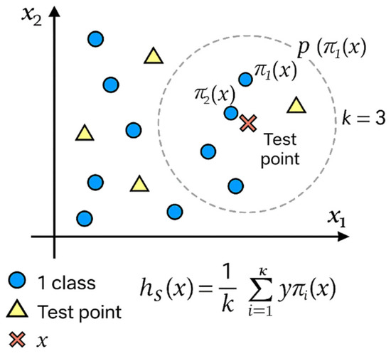
Figure 3.
Illustration of the KNN algorithm with k = 3.
2.4.2. XGBoost
XGBoost is a supervised learning algorithm based on decision trees. It is considered one of the highest-performing algorithms in the evolution of tree-based techniques due to its optimized sequential ensemble approach. XGBoost employs a gradient boosting method that enables the construction of decision trees in a sequential manner, each aiming to progressively reduce the prediction error [42]. The XGBoost algorithm offers several key features that distinguish it from other decision tree-based algorithms such as Random Forest:
- Sequential Ensemble (CART): XGBoost uses an ensemble of decision trees built sequentially under the CART (Classification and Regression Trees) framework. In this approach, each new tree learns from the errors made by previous trees and refines its predictions through a process known as gradient descent. This iterative optimization corrects accumulated errors, thereby improving the model’s accuracy at each step. As more trees are added, the model incrementally minimizes the loss function, such as mean squared error, leading to a better fit to the data [43].
- Tree Depth Control: Unlike Random Forest, where trees grow to their maximum depth, XGBoost allows the user to define a maximum tree depth. This helps to control model complexity and prevents overfitting [43].
- Parallel Processing: XGBoost is designed to take advantage of parallel computing capabilities, enabling highly efficient model training. This is particularly valuable for large datasets, significantly reducing training time [43].
- Regularization: XGBoost incorporates regularization terms that penalize model complexity, helping to mitigate overfitting. This adds an additional balance between accuracy and the model’s generalization capacity [43].
- Handling of Missing Values: The algorithm includes mechanisms to automatically manage missing values in the dataset, directing them to the most appropriate branch in the decision trees, which enhances model accuracy and robustness [43].
The learning process of XGBoost is structured as a series of iterative stages, as illustrated in Figure 4, where new trees are trained on residuals from previous iterations. This stepwise approach progressively improves prediction accuracy. The final predictive function is constructed as the additive sum of base learners, each minimizing the loss at its respective stage [44]:
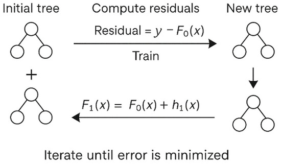
Figure 4.
Conceptual representation of the XGBoost learning process.
- Initial Tree: The process begins with the construction of an initial tree, , which provides an initial prediction of the target variable, . This tree produces a residual, defined as the difference between the actual value and the prediction ;
- Subsequent Tree Construction: A second tree, , is trained to fit the residual errors of the initial tree . The goal is for to learn the residuals and, when combined with , reduce the overall model error;
- Tree Combination: Trees and are combined to form a new model , which reduces the mean squared error compared to . This is expressed as:where represents the updated prediction function after adding a correction term, is the initial base function, possibly a preliminary model or a prior iteration and is the adjustment or improvement term added in this step.
- Iteration Until Error Minimization: This process continues iteratively until the final model is obtained, which minimizes the error as much as possible. Each iteration adds a new tree that fits the residuals of the previous iteration:where is the prediction function at the current iteration m, representing the improved model, is the function from the previous iteration, serving as the base for the current update, and is the correction or improvement term added during iteration , typically based on current data or residual errors.
2.4.3. LSTM
LSTM is an advanced type of recurrent neural network specifically designed to handle sequential prediction tasks, particularly those involving long-duration data such as time series or natural language. What sets LSTM apart is its built-in memory mechanism, which enables the model to retain relevant information across multiple processing steps. This capability effectively addresses one of the major limitations of traditional RNNs, the vanishing or exploding gradient problem, by allowing the network to learn and preserve long-term dependencies in the data [45].
Structurally, an LSTM uses three key “gates” in each cell: the forget gate, the input gate, and the output gate. These gates act as filters that control the flow of information through the cell, allowing the network to selectively store or discard information. The forget gate determines what information should be removed from the cell, based on the current input and previous state, generating a value between 0 and 1 (with 1 indicating that the information should be retained). The input gate controls what new information will be added to the cell state and uses the Tanh function to create candidate values for storage. Finally, the output gate determines the information that will be sent to the next state, adjusting the cell state value within a range of −1 to 1 and modulating it for the current output [46].
The LSTM structure enables the network to accumulate relevant knowledge over an extended sequence, facilitating sequential prediction tasks such as machine translation, text summarization, and response generation in question-answering systems. Thanks to its ability to handle both short- and long-term learning, LSTM is applied in environments such as time series analysis, where the model adapts to understand complex patterns and dependencies in the data. This makes it ideal for prediction applications in domains such as economics and meteorology, where historical data sequences directly influence future forecasts [46].
The LSTM architecture is based on a structure that enables information to flow through a cell via a memory mechanism controlled by three gates: the forget gate, the input gate, and the output gate. These gates operate in coordination to control what information should be retained or discarded at each time step of the sequence, allowing the network to learn long-term dependencies. Figure 5 graphically represents the internal architecture of an LSTM cell, illustrating the forget, input, and output gates, as well as the activation and combination operations that allow the cell state to be maintained and updated.
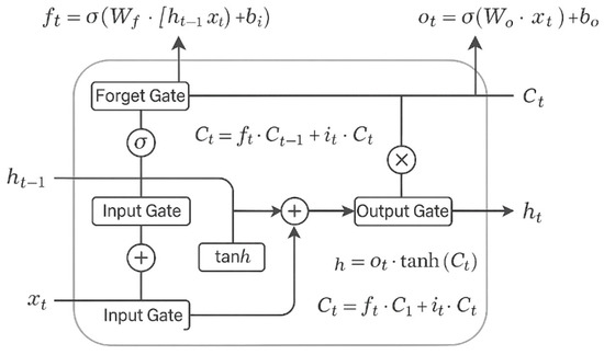
Figure 5.
Internal architecture of an LSTM cell.
- Forget Gate (): This gate determines how much of the previous cell state should be retained. It is mathematically defined as:where is the weight matrix associated with the forget gate, is the bias, is the output of the previous cell, is the current input, and is the sigmoid activation function, which outputs values between 0 and 1. A value close to 1 indicates that the previous information should be preserved.
- Input Gate (): This gate decides what new information will be added to the cell state. It consists of two components: the activation of the input gate and the generation of the candidate cell state (), representing new information to potentially be stored. These are computed as follows:where and are weight matrices, and are the biases, and tanh is the hyperbolic tangent activation function, which outputs values between −1 and 1 to produce candidates for the new state.
- Cell State Update (): The new cell state is computed by combining the retained information (regulated by ) and the new candidate state (regulated by ). The update is performed as:where (⋅) denotes element-wise multiplication. This operation ensures that relevant past information is preserved while incorporating new insights.
- Output Gate (): This gate determines which part of the cell state will be used as the cell’s output , which is then passed to the next time step and serves as the current output:where is the weight matrix and is the output gate bias.
- Cell Output (): The output is calculated by applying the function to the updated cell state , modulated by the output gate :
This output is passed to the next time step, enabling information to flow across time steps and maintain continuity, thus creating the “memory effect” characteristic of LSTM networks [46].
2.4.4. Random Forest
The Random Forest algorithm, introduced by Leo Breiman in 2001 [47], is an ensemble learning technique that combines multiple decision trees to enhance the accuracy and robustness of predictions in classification and regression tasks. This methodology relies on constructing a collection of decision trees, each trained on a random sample of the original dataset using the “bootstrap aggregating” or “bagging” method [47].
The Random Forest algorithm, widely used in classification and regression tasks, is based on a solid mathematical approach to addressing prediction problems. Consider a training dataset defined as , where represents the feature vector associated with example i, consisting of attributes, and is the corresponding label. This label can either be an element of a discrete set (in the case of classification) or a continuous value (in the case of regression). The fundamental objective is to learn a function that enables the prediction of Y from X with the smallest possible error. Formally, the problem is posed as the minimization of the expected error [48].
where is a loss function that measures the discrepancy between the prediction ynd the true value , and denotes the joint distribution of the variables and . This general framework applies to both classification tasks, where the typical loss function is cross-entropy, and regression tasks, where the mean squared error is commonly employed [48].
The construction of trees in the Random Forest algorithm follows a structured process aimed at maximizing the diversity among individual models and enhancing their generalization ability. This process involves three fundamental steps: generating data subsets through the bootstrap method, randomly selecting features at each node, and determining the best split at each node.
The first step, known as bootstrap sampling, consists of generating training subsets from the original dataset . This procedure is performed via sampling with replacement, meaning that some observations may appear multiple times within a subset, while others may not be included at all. Each subset contains approximately observations, ensuring that all trees have access to representative data, while incorporating slight variations to promote diversity. In the second step, during the construction of each tree , a random feature selection mechanism is introduced.
At each node, a random subset of features ( selected from the available features. This procedure ensures that trees do not rely solely on a fixed set of attributes, thereby reducing the correlation among them and increasing the robustness of the ensemble model. The third step focuses on the splitting of tree nodes. For each node, a quality metric , is evaluated, which may be entropy or the Gini index for classification problems or mean squared error for regression tasks. If the node contains a subset of data , goal is to identify the attribute and threshold that maximize the information gain. This gain is formally defined as [49]:
where and are the resulting subsets after splitting by attribute and threshold , and denotes a measure of impurity (such as entropy or the Gini index). This calculation ensures that the splits performed within the tree maximize the purity of the resulting subsets, thereby enhancing the predictive capability of the model.
Once the trees that comprise the Random Forest model have been trained, the prediction process aggregates the individual outputs of these trees to produce a more robust final result. This process varies depending on whether the task is classification or regression, but in both cases, it relies on the aggregation of predictions from the individual trees. In classification tasks, each tree generates a class prediction for a new data point . The final prediction of the model is determined by majority voting among all tree predictions. Mathematically, the final predicted class is the one that receives the greatest number of votes [49]:
where is the indicator function, which takes the value 1 if the condition inside the parentheses is satisfied, and 0 otherwise. This approach ensures that the most represented class among the trees is selected as the final prediction, thereby helping to mitigate errors arising from inaccurate individual decisions. In the case of regression problems, each tree provides a continuous value for the data point . The final prediction of the Random Forest is computed as the average of these individual predictions [49]:
This averaging process reduces the variance of individual predictions, providing a more stable and accurate estimate compared to using a single decision tree. In both cases, the aggregation process is fundamental for leveraging the diversity of the trees within the model. By combining multiple predictions, Random Forest becomes more robust against overfitting and potential irregularities in the training data, thereby enhancing the generalization capability of the final model. Figure 6 presents a schematic representation of the algorithm, illustrating multiple decision trees trained on bootstrap subsets of the original dataset, whose individual predictions are aggregated through averaging to obtain the final prediction.
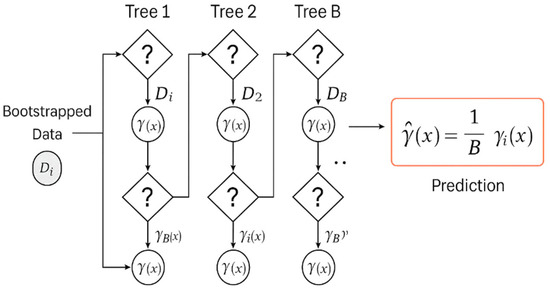
Figure 6.
Schematic Representation of the Random Forest Algorithm.
2.4.5. Model Overview, Strengths and Limitations
This section presents a concise overview of how each algorithm operates in regression tasks, emphasizing the key characteristics most relevant to the forecasting problem under study. The main features of each model are summarized below.
- KNN: This is a non-parametric, instance-based algorithm that performs regression by estimating the output of a new observation based on the values of its k nearest neighbors in the training set. It uses distance metrics such as Euclidean or Manhattan distance to identify the closest data points in the feature space, under the assumption that instances located near each other tend to have similar target values. In its weighted versions, closer neighbors have a greater influence on the prediction, which enhances accuracy in dense or heterogeneous regions. Since KNN does not involve a formal training phase, it is simple to implement; however, it can be computationally expensive at prediction time and is sensitive to noise and high-dimensional data.
- Random Forest: This algorithm is an ensemble regression method that constructs multiple decision trees using bootstrap sampling and random feature selection and then aggregates their predictions through averaging. Since each tree is trained on a different subset of the data and considers a random subset of features, the resulting model captures diverse patterns, which enhances generalization and reduces the risk of overfitting. By combining numerous weak learners, Random Forest achieves greater robustness and provides stable predictions even in the presence of noisy or complex datasets. Its main strength lies in its ability to model nonlinear relationships and variable interactions; however, it does not incorporate any inherent mechanism to capture temporal dependencies.
- XGBoost: A regression algorithm that builds decision trees sequentially, where each new tree is trained to correct the residual errors of the previous ones. This gradient boosting process minimizes a loss function, such as mean squared error, through iterative optimization. XGBoost includes advanced features such as regularization to prevent overfitting, parallel processing to speed up computation, and the ability to handle missing values efficiently. As a result, it produces highly accurate models for tabular and heterogeneous data, though it tends to reproduce dominant patterns rather than long-term temporal dynamics.
- LSTM: A type of recurrent neural network specifically designed to capture sequential dependencies in time-series data. Each LSTM cell incorporates three gates: forget, input, and output, which regulate how information is retained, updated, or discarded over time. This mechanism allows the network to preserve relevant signals across time steps and helps mitigate the vanishing gradient problem. In regression tasks, LSTM predicts continuous values by learning long-term temporal patterns. This makes it particularly effective in dynamic environments where future outcomes depend heavily on historical sequences, such as flight trajectories.
Additionally, Table 2 provides a comparative analysis of the selected models, focusing on their strengths and weaknesses in regression scenarios, especially when applied to complex variables involving temporal dependencies.

Table 2.
Strengths and weaknesses of the selected models in forecasting tasks.
2.5. Model Performance Evaluation
The assessment of model performance for three-dimensional airspace occupancy prediction constituted a critical stage of the methodological validation process. To this end, quantitative metrics were applied to both training and validation datasets with the objective of estimating accuracy, generalization capacity, and explanatory robustness of the algorithms. The primary indicators selected were the Mean Absolute Error (MAE), the Root Mean Squared Error (RMSE), and the Coefficient of Determination (R2), which are commonly employed in predictive modeling [50].
To broaden the analysis, additional measures were incorporated: the Pearson Correlation Coefficient (R), used to quantify the linear relationship between observed and predicted values; the Mean Absolute Percentage Error (MAPE), which expresses error in relative terms and facilitates percentage-based interpretation for continuous variables; the Scatter Index (SI), defined as the ratio of RMSE to the mean of observed values; and the Discrepancy Ratio (DR), computed as the ratio of the sum of predicted values to the sum of observed values, serving as an indicator of systematic bias [51].
In addition to these numerical metrics, graphical representations such as scatter plots, violin plots, and heatmaps were included for both training and validation phases. These visualizations were employed to examine the distribution of residuals, detect potential biases, and evaluate the spatiotemporal coherence of predictions. The combination of numerical and graphical approaches provided an integrated framework for model comparison and enabled the identification of overfitting or underfitting phenomena [52].
Table 3 summarizes the units associated with each metric as applied to the output variables of the predictive models (latitude, longitude, and altitude). The table highlights that error measures (MAE and RMSE) preserve the original units of the predicted variables, while relative and dimensionless metrics (R2, R, MAPE, SI, DR) facilitate cross-model comparisons. This distinction is essential to ensure that both the magnitude of prediction errors and their proportional significance are adequately interpreted.

Table 3.
Units of evaluation metrics applied to output variables (latitude, longitude, and altitude).
2.5.1. Mean Absolute Error (MAE)
The MAE quantifies the average absolute error between the model’s predictions and the observed true values. It is an easily interpretable metric, as it retains the original units of the target variable. It is defined as:
where represents the true values, the values predicted by the model, and the total number of observations. The MAE provides a robust measure against small variations; however, it does not differentially penalize large errors, which can be a limitation in contexts sensitive to extreme deviations [53].
2.5.2. Root Mean Squared Error (RMSE)
The RMSE measures the magnitude of the mean squared error between predictions and true values, penalizing large errors more heavily due to the squaring operation. It is calculated as:
This metric is more sensitive to outliers and provides an indication of the average deviation expected between the predictions and the actual values. In this study, a low RMSE indicated a high degree of accuracy in predicting airspace density [53].
2.5.3. Coefficient of Determination (R2)
The Coefficient of Determination (R2) is a statistical metric that represents the proportion of the total variability of the dependent variable that can be explained by the regression model. It is expressed by the following equation:
where represents the mean of the observed values. An R2 value close to 1 indicates that the model has a high explanatory capacity, whereas values near 0 reveal that the model explains little variability in the data. Nevertheless, this metric can be misleading if the model is overfitted or if the relationship between variables is not linear; therefore, it was used in conjunction with other metrics.
2.5.4. Pearson Correlation Coefficient (R)
The Pearson correlation coefficient (R) measures the strength and direction of the linear relationship between the observed values and the predicted values. It ranges be-tween −1 and 1, where values close to 1 indicate a strong positive correlation, values close to −1 a strong negative correlation, and values near 0 indicate no linear correlation. It is defined as:
where are the observed values, are the predicted values, is the mean of the observed values, and is the mean of the predicted values. Unlike R2, this metric directly assesses the linear association between the two variables, making it useful for verifying whether the model captures proportional changes. However, it is sensitive to outliers, which can distort the correlation value [54].
2.5.5. Mean Absolute Percentage Error (MAPE)
The Mean Absolute Percentage Error (MAPE) expresses the prediction error as a percentage of the observed values, making it an intuitive and scale-independent measure. It is defined as:
where are the observed values, are the predicted values, and n is the number of observations. MAPE is advantageous because it provides a relative error measure that is easy to interpret. Nevertheless, it cannot be applied when , and it tends to overemphasize errors when observed values are very small [53].
2.5.6. Mean Absolute Percentage Error (MAPE)
The Scatter Index (SI) is a normalized error metric that relates the root mean squared error (RMSE) to the mean of the observed values. It enables comparison of prediction accuracy across datasets with different scales. It is expressed as:
where RMSE is the root mean squared error and is the mean of the observed values. SI provides a dimensionless measure that facilitates relative error comparison. A lower SI indicates higher predictive accuracy. This metric is commonly applied in environmental modeling and atmospheric sciences to assess relative forecast skill [55].
2.5.7. Discrepancy Ratio (DR)
The Discrepancy Ratio (DR) evaluates whether the model systematically overestimates or underestimates the predictions. It is computed as the ratio of the sum of predicted values to the sum of observed values:
where are the observed values and the predicted values. A value of indicates that the model is unbiased, while suggests overestimation and indicates underestimation. Although useful for detecting global bias, DR does not provide information about the magnitude or distribution of individual prediction errors [56].
2.5.8. Complementary Visualizations
In addition to numerical metrics, graphical tools were incorporated to provide deeper insights into the distribution of errors and the consistency of the predictive models. Three types of visualizations were selected: dispersion plots, violin plots, and heat maps, each offering complementary perspectives on model performance.
Dispersion plots were employed to contrast observed versus predicted values in both the training and validation phases. These plots make it possible to visually identify systematic deviations, clustering patterns, and potential outliers that might not be evident from global error metrics alone [57].
Violin plots were used to characterize the distribution of residuals across the models. By combining box plot summaries with kernel density estimations, violin plots provide a clear depiction of bias, variability, and the presence of asymmetric error distributions, which are critical for understanding the robustness of the algorithms [54].
Heat maps were implemented to visualize the density and intensity of prediction errors. By mapping residual magnitudes across two dimensions, such as observed versus predicted values or errors over time, heat maps facilitate the detection of systematic overestimation or underestimation and highlight regions where errors concentrate, thereby complementing both dispersion and violin plots [58].
3. Results and Analysis
3.1. Data Preparation
The initial dataset employed in this study consisted of 67,984,768 observations corresponding to flight records within Colombian airspace. The dataset included essential variables for the three-dimensional characterization of air traffic, such as flight identification (airline and flight number), date and time in both UTC and local formats, as well as positional parameters (latitude, longitude), flight level expressed in feet, speed, heading, and various quality indicators associated with ADS-B reports.
A series of rigorous data-cleaning procedures was implemented to ensure consistency and validity. First, records missing any of the three fundamental parameters for prediction, latitude, longitude, or altitude, were removed. These cases accounted for less than 5% of the total and did not significantly affect spatial or temporal coverage. Next, duplicate records arising from redundant transmissions within short intervals were identified and discarded, eliminating approximately 3.7% of the dataset. In addition, outlier detection was carried out to exclude observations with altitudes below zero feet or above FL600, as well as geographic coordinates outside the valid limits of latitude (±90°) and longitude (±180°). This procedure affected about 1.8% of the data and reduced the influence of spurious information during model training.
After these filtering stages, the final dataset comprised approximately 61,184,000 valid observations, representing around 90% of the original volume. This remaining dataset provided a sufficiently broad and representative sample of actual air traffic behavior in Colombia, preserving both temporal variability and spatial dispersion of trajectories. Consequently, the predictive models were trained on high-quality information, minimizing bias and enhancing the robustness of the results.
Once the proposed models were trained and validated, their performance was evaluated on the specific task of forecasting three-dimensional airspace occupancy over Colombian territory. The assessment focused on comparing the accuracy and generalization capacity of KNN, Random Forest, XGBoost, and LSTM, using quantitative metrics such as MAE, RMSE, and the Coefficient of Determination (R2), complemented by additional indicators including R, MAPE, SI, and DR. The analysis emphasized how each model performed under varying data volumes and traffic conditions, highlighting their effectiveness in scenarios characterized by high-density flows. The results provided a clear basis for determining which algorithm is best suited to support planning and operational forecasting within the framework of Trajectory-Based Operations.
3.2. KNN
The K-Nearest Neighbors (KNN) regressor was implemented using the scikit-learn library (v1.4) in Python 3.9, with the objective of predicting latitude, longitude, and flight level simultaneously. The most critical hyperparameter in this model is the number of neighbors (n_neighbors), which directly controls the balance between local sensitivity and generalization. An exploratory search was conducted in the range of 1–20 and subsequently extended to higher values to evaluate smoothing effects. The optimal configuration was obtained with k = 200, which allowed the model to reduce noise sensitivity while avoiding excessive over smoothing of spatial patterns.
The Euclidean distance metric (L2 norm) was chosen to compute proximity, as it provides reliable performance when dealing with continuous geospatial variables. Predictions were generated using uniform weighting, meaning that all neighbors contributed equally to the final estimate. This configuration yielded more consistent outcomes than distance-based weighting schemes, which in preliminary tests introduced unnecessary variability across different flight regions. For the neighbor search algorithm, the auto setting was retained, enabling the library to dynamically select between ball-tree, kd-tree, or brute-force search depending on the dataset structure. The leaf size parameter was fixed at 30, since sensitivity analyses demonstrated negligible influence on prediction accuracy. Finally, multi-core execution was enabled with n_jobs = −1, substantially reducing computation time during neighborhood queries.
Unlike parametric models, KNN does not construct an explicit functional mapping between predictors and outputs. Instead, it relies on memory-based storage of training instances and produces predictions by averaging the target values of the nearest neighbors. This characteristic limit its ability to capture sequential or nonlinear dependencies, such as those present in temporal air traffic dynamics. However, it provides robustness and interpretability in local spatial relationships, making it a suitable baseline for evaluating predictive tasks in three-dimensional airspace occupancy.
Figure 7 shows an example of the predictions generated by the KNN model. In the first image, the predicted points are projected onto a two-dimensional map of Colombia, allowing the spatial distribution of predictions to be observed. A higher concentration of points is evident in the central region, where the historical data density is greater.
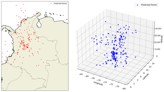
Figure 7.
Prediction by the KNN Algorithm.
The second image represents the predictions in three-dimensional space, incorporating altitude as a third dimension. In this case, it can be seen that the predictions tend to cluster vertically, reflecting the non-parametric, neighborhood-based nature of the model. This representation also highlights the model’s limited ability to capture complex structures in altitude, as predictions are adjusted based on the local density of previous examples without considering sequential dynamics. These visualizations reinforce the understanding of the model’s behavior, showing both its relative effectiveness in planar coordinates and its limitations in more sensitive variables such as flight level.
Figure 8 illustrates the performance of the KNN model through scatter plots of observed versus predicted values. For latitude and longitude, shown in Figure 8a–d, the points are widely dispersed and reveal only a weak alignment with the identity line, indicating limited predictive capacity. In Figure 8e–f, corresponding to flight level, the deviations become more pronounced, with predicted values spread vertically across a broad range. The figure highlights the model’s sensitivity to local variations and its lack of robustness in capturing the nonlinear and sequential patterns required for accurate air traffic prediction.
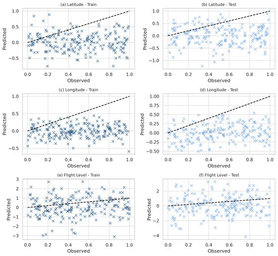
Figure 8.
Scatter plots of observed versus predicted values for the KNN model: (a) Latitude-Train, (b) Latitude-Test, (c) Longitude-Train, (d) Longitude-Test, (e) Flight Level-Train, (f) Flight Level-Test.
3.3. XGBoost
The gradient-boosted decision tree model (XGBoost) was implemented in Python using the xgboost library as a multi-output regressor to predict latitude, longitude, and flight level. Model capacity and regularization were controlled primarily through the number of boosting iterations, tree depth, and stochastic sampling. The final configuration comprised 500 trees with a maximum depth of 6 and a learning rate of 0.05, a combination that enabled gradual function fitting while limiting over-correction between successive learners. Each tree was trained on a row subsample of 0.8 (subsample = 0.8) and a column subsample of 0.8 at the tree level (colsample_bytree = 0.8), introducing stochasticity to decorrelate learners, reduce variance, and mitigate overfitting. A fixed random seed (random_state = 42) was used to ensure reproducibility.
Hyperparameter selection followed an iterative cross-validation procedure in which candidate settings were compared using mean squared error (MSE) as the selection criterion. This loss function was also adopted during training to emphasize penalization of large deviations, a desirable property for altitude forecasting and other safety-critical outputs. In the adopted setup, XGBoost uses additive tree updates and second-order optimization, which together support stable convergence under moderate learning rates. The chosen depth = 6 provided sufficient representational power for nonlinear interactions without incurring the instability commonly observed with deeper trees in noisy regimes, while the subsample/colsample pair-controlled learner diversity and acted as an implicit regularized.
The resulting estimator thus balances bias and variance through (i) conservative learning rate and depth, (ii) a sufficient number of boosting rounds to capture residual structure, and (iii) stochastic sampling to improve generalization. All experiments were conducted in Python with xgboost for model training and NumPy/pandas/Matplotlib for data handling and reporting. If desired, early stopping on a held-out validation fold (e.g., early_stopping_rounds) can be added to this configuration without altering the core hyperparameter choices documented above.
Figure 9 presents a representative example of the predictions generated by the XGBoost model for flights operating within Colombian airspace. In the two-dimensional (2D) visualization, the predicted points appear densely concentrated within a relatively small geographic region, indicating the model’s tendency to reproduce the dominant patterns observed in the training data. This clustering suggests a limited capacity for spatial generalization, likely due to the model’s focus on frequently traveled trajectories.
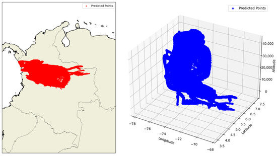
Figure 9.
Prediction by the XGBoost Algorithm.
In the 3D projection, which integrates altitude alongside latitude and longitude, the clustering becomes even more apparent. Predicted flight positions are tightly grouped along a narrow vertical range, with minimal lateral dispersion across different altitudes. This pattern points to a limitation in the model’s ability to represent the vertical structure of the airspace and the continuity of real-world flight paths, despite the implementation of regularization and subsampling mechanisms. These findings suggest that while XGBoost performs well in capturing prominent trends, it faces challenges in modeling the full complexity of three-dimensional air traffic behavior.
As presented in Figure 10, the scatter plots of the XGBoost model show only partial improvement compared to KNN. Figure 10a–d, which represent latitude and longitude, demonstrate a slightly closer grouping of predictions around the identity line, although large deviations remain visible. Figure 10e–f, corresponding to flight level, reveal highly scattered predictions with limited correlation to the observed values. This figure underscores the difficulty of gradient-boosted trees in modeling altitude and sequential dynamics, despite their modest gains in horizontal coordinates.
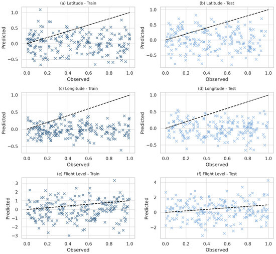
Figure 10.
Scatter plots of observed versus predicted values for the XGBoost model: (a) Latitude-Train, (b) Latitude-Test, (c) Longitude-Train, (d) Longitude-Test, (e) Flight Level-Train, (f) Flight Level-Test.
3.4. Random Forest
The Random Forest model was trained by selecting an appropriate number of decision trees to strike a balance between prediction accuracy and computational efficiency. In this case, the ensemble was composed of 100 trees, a configuration widely supported in the literature for its ability to yield reliable results without imposing significant execution time. As the number of trees in a Random Forest increases, the variance of the predictions typically decreases, since the averaging process helps to smooth out the errors made by individual trees. However, beyond a certain threshold, adding more trees results in diminishing returns while significantly increasing the use of computational resources. For this reason, the chosen number represents a practical compromise between model robustness and operational feasibility.
Each tree in the ensemble was trained on a randomly selected subset of the original dataset, generated through a resampling technique known as bootstrap aggregating or bagging. This method introduces variability across the trees by allowing each to learn from a different sample of the data, promoting the exploration of diverse partitions within the feature space. As a result, the model becomes better equipped to recognize a broader range of patterns, and the risk of overfitting often present in individual decision trees is significantly reduced. In addition to instance resampling, the model applied random feature selection at each decision node during the construction of the trees. This technique ensures that not all trees are influenced by the same dominant variables, which is particularly useful in high-dimensional datasets or in cases where variables are strongly correlated. The combined effect of bagging and randomized feature selection leads to an ensemble of diverse decision trees that, when aggregated through averaging, produce more stable and generalizable predictions.
Figure 11 illustrates a representative example of the predictions generated by the Random Forest model for a specific date and time. In the 2D geographic visualization, only a single predicted point appears over Colombian territory, suggesting an extremely localized response by the model. This lack of spatial dispersion is consistent with the results observed in earlier 3D projections, where predictions exhibited limited altitude variability and a tendency to reproduce patterns seen in the training data, with minimal capacity for extrapolation. Such behavior reflects the model’s limited adaptability to new temporal configurations. This is likely due to the inherent structure of Random Forest, which, while powerful for many tasks, does not explicitly incorporate sequential or time-dependent information. Unlike models designed to capture temporal evolution, Random Forest operates on static input-output relationships, without modeling the continuity or progression of events over time.
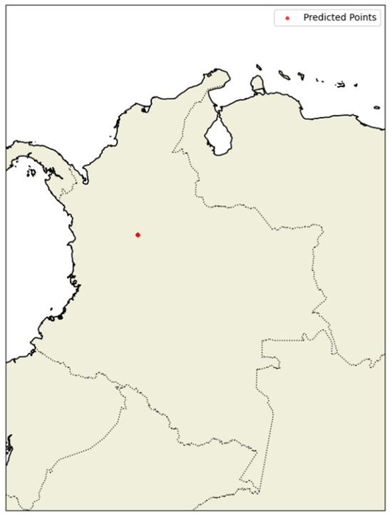
Figure 11.
Prediction by the Random Forest Algorithm.
Although this architecture offers notable robustness and is effective for many classification and regression tasks, its utility is constrained in aeronautical contexts that require a dynamic understanding of multidimensional trajectories. Consequently, while Random Forest can serve as a solid baseline for performance comparison, it is not the most effective choice for representing the complex and evolving dynamics of air traffic in 3D space.
Figure 12 depicts the scatter plots for the Random Forest model, showing considerable error dispersion across all variables. In panels (a–d), corresponding to latitude and longitude, the predictions deviate substantially from the identity line, reflecting weak explanatory power. Panels (e–f) highlight the model’s performance in predicting flight level, where residuals increase sharply, and predictions fail to capture the true altitude behavior. The figure emphasizes the limitations of Random Forest in addressing the complexity of three-dimensional air traffic data, particularly when temporal dependencies play a central role.
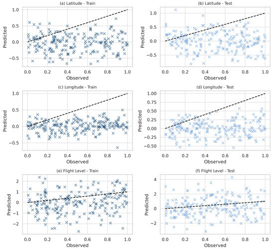
Figure 12.
Scatter plots of observed versus predicted values for the Random Forest model: (a) Latitude-Train, (b) Latitude-Test, (c) Longitude-Train, (d) Longitude-Test, (e) Flight Level-Train, (f) Flight Level-Test.
3.5. LSTM
The LSTM network was implemented in Python using TensorFlow/Keras as a multivariate regressor with three continuous outputs (latitude, longitude, flight level). The architecture comprised two stacked LSTM layers followed by a fully connected head: an LSTM layer with 64 units and return_sequences = True, a second LSTM layer with 32 units and return_sequences = False, a Dense(32) hidden layer with ReLU activation, and a linear output layer Dense(3) mapping to the target variables. The LSTM cells used the standard Keras activations—tanh for the cell/output and sigmoid for the gates—with default orthogonal recurrent initialization. No dropout or recurrent dropout was applied in this configuration.
Inputs to the network were organized as sequences with a single time step and a feature vector derived from cyclic temporal encodings that had been scaled to 0.1 and projected with PCA to 6 components. Accordingly, the training tensors had shape (N, 1, 6) and the targets had shape (N, 3). The model was optimized with Adam (Keras default settings) under an MSE loss, which emphasizes large deviations in continuous regression and is appropriate for safety-critical altitude prediction. Training was conducted with a batch size of 64 for 1 epoch on the prepared split (code-level configuration), and a held-out validation set was used to monitor generalization. The final layer’s linear activation preserved the physical scale of the outputs, avoiding implicit bounding that could bias latitude/longitude or flight-level predictions.
At inference, the code implements a recursive one-step-ahead strategy to produce a fixed-length trajectory: given an initial feature vector, the network generates a prediction, updates the cyclic temporal features deterministically (day/hour/minute phases), and repeats for 150 steps. Predictions are therefore obtained by iterating the learned one-step mapping with externally advanced temporal features and are returned as a sequence of 3D waypoints suitable for downstream visualization (2D map and 3D plots). All experiments for this model were executed in Python (TensorFlow/Keras), with NumPy/pandas for data handling and Matplotlib/Cartopy for visualization.
The results of this model are shown in Figure 13, where both the geographic 2D and 3D predictions generated by the LSTM network are presented. On the map of Colombia, the predicted points are widely and realistically distributed across the national airspace, demonstrating the model’s adequate capacity to generalize across diverse regions and capture the operational dynamics of flights. The 3D visualization, in turn, shows a coherent and well-structured dispersion of points along the longitude, latitude, and altitude axes, validating the model’s ability to represent complete and differentiated trajectories in altitude.
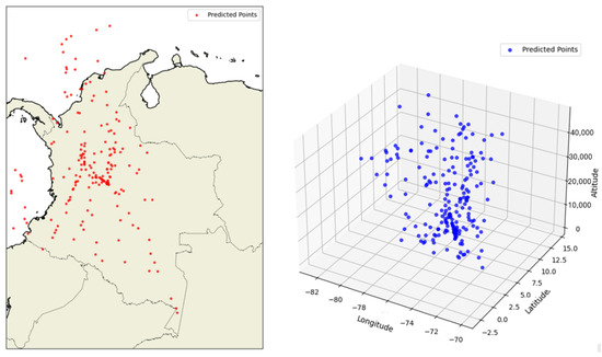
Figure 13.
Prediction by the LSTM algorithm.
Figure 14 presents the scatter plots for the LSTM model, which demonstrate a clear improvement in predictive accuracy compared to non-sequential approaches. Figure 14a–d, show that for latitude and longitude, the predictions follow the identity line more closely, with reduced variability and tighter clustering of points. Figure 14e–f, representing flight level, confirm the model’s strong ability to reproduce altitude values with minimal dispersion. The figure illustrates the LSTM’s advantage in capturing temporal dependencies and nonlinear structures, establishing it as the most effective model for three-dimensional trajectory prediction.
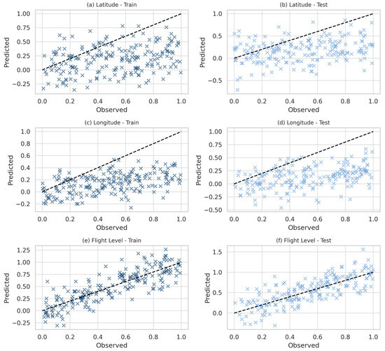
Figure 14.
Scatter plots of observed versus predicted values for the LSTM model: (a) Latitude-Train, (b) Latitude-Test, (c) Longitude-Train, (d) Longitude-Test, (e) Flight Level-Train, (f) Flight Level-Test.
3.6. Model Comparison
The comparative evaluation of the models developed in this study made it possible to identify the specific strengths and limitations of each approach in the context of three-dimensional air trajectory prediction. The results highlight how different algorithms respond to the challenges posed by sequential spatial data and varying traffic conditions.
Figure 15 presents the evaluation outcomes through grouped bar plots, where the metrics are displayed for both the training and validation phases, thus allowing a direct comparison of predictive performance across models. The set of evaluation indicators includes the MAE, RMSE, and the R2, complemented by additional measures that provide a more detailed assessment.
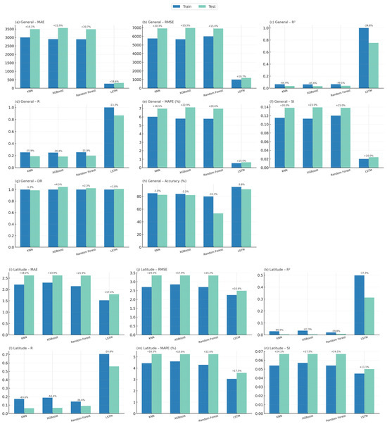
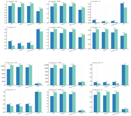
Figure 15.
Comparative evaluation of predictive models using grouped bar plots for training and validation phases. The figure presents the following metrics: (a) MAE (General), (b) RMSE (General), (c) R2 (General), (d) R (General), (e) MAPE (General), (f) SI (General), (g) Discrepancy Ratio (General), (h) Accuracy (General), (i) MAE (Latitude), (j) RMSE (Latitude), (k) R2 (Latitude), (l) R (Latitude), (m) MAPE (Latitude), (n) SI (Latitude), (o) MAE (Longitude), (p) RMSE (Longitude), (q) R2 (Longitude), (r) R (Longitude), (s) MAPE (Longitude), (t) SI (Longitude), (u) MAE (Flight Level), (v) RMSE (Flight Level), (w) R2 (Flight Level), (x) R (Flight Level), (y) MAPE (Flight Level), and (z) SI (Flight Level). Results are reported for the KNN, XGBoost, Random Forest, and LSTM models. Each subplot displays the performance for training (blue) and validation (green) phases, with the percentage difference between them annotated above each pair of bars, thus facilitating a direct assessment of model generalization and robustness.
These comprise the R, which captures the linear association between predicted and observed values; the MAPE, which expresses the error magnitude in relative terms; the SI, which normalizes the RMSE by the mean of observed values; and the DR, which detects global tendencies of systematic overestimation or underestimation. The inclusion of percentage differences between training and validation phases in the plots further enhances interpretability, making it possible to detect signs of overfitting or underfitting in each algorithm. Overall, the combined use of numerical metrics and visual comparison in Figure 15 provides a rigorous and comprehensive framework to evaluate model performance, supporting an objective analysis of their suitability for trajectory-based planning and strategic airspace management.
The results presented in Figure 15 clearly demonstrate that the LSTM model consistently achieves superior predictive performance across all evaluation metrics and variables. In terms of overall error magnitude, LSTM delivers an MAE of 312.59 and a RMSE of 1187.43, values that are markedly lower than those obtained by KNN, XGBoost, and Random Forest, whose errors remain above 3400 for MAE and 6800 for RMSE. The R2 for LSTM reaches 0.7523, indicating that the model explains more than 75% of the variance in the data, while the traditional approaches fail to exceed 4%, confirming their inability to capture the underlying dynamics of the problem.
The inclusion of complementary metrics provides further insight into these differences. The R for LSTM remains consistently high across all variables (up to 0.99 for flight level), whereas the alternative models exhibit values below 0.3, confirming weak linear associations between observed and predicted values. Similarly, the MAPE for LSTM remains close to or below 3–4% in latitude, longitude, and flight level, while the other models often exceed 30% for flight level. The SI also highlights this contrast: LSTM achieves normalized error ratios close to 0.02–0.07, compared to values near 0.4 for the traditional algorithms. Importantly, the DR for LSTM remains near unity, confirming the absence of systematic overestimation or underestimation, while tree-based models exhibit larger deviations.
For latitude and longitude, although all models yield relatively low absolute errors, LSTM achieves further reductions while substantially improving explanatory power, with R2 values of 0.3125 and 0.2857, respectively. This suggests that LSTM not only minimizes error but also more effectively captures the spatial structure of the data. The advantage of LSTM becomes particularly evident when predicting flight level, a variable of critical operational importance. LSTM reaches an MAE of 978.53 and an R2 of 0.9854, showing its capacity to learn and reproduce nonlinear sequential patterns in vertical airspace dynamics. In contrast, the other models produce R2 values below 0.1, underscoring their limitations in modeling altitude.
The comparative bar plots also reveal the differences between training and validation phases. While tree-based models (KNN, XGBoost, Random Forest) display relatively large increases in error from training to validation, indicating weak generalization, the LSTM maintains stable performance, with percentage differences consistently small across all metrics. This highlights its robustness against overfitting.
Finally, the normalized accuracy derived from MAE reinforces these findings: LSTM achieves 91.36%, followed by KNN and XGBoost (≈82%), while Random Forest lags significantly at just above 53%. The results confirm that although KNN and XGBoost may appear acceptable in simpler dimensions such as latitude and longitude, they fail to generalize to the more complex prediction of flight level. Overall, the evidence underscores the importance of using models such as LSTM that are capable of learning sequential dependencies and nonlinear relationships in multidimensional airspace data.
The graphical results presented in Figure 15 reveal a consistent pattern across all evaluated dimensions. Models without sequential processing capabilities, such as KNN, XGBoost, and Random Forest, exhibit limited capacity to capture the temporal dependencies inherent in air traffic data. Although KNN and XGBoost achieve acceptable performance in variables with relatively low variability, such as latitude and longitude, their errors increase substantially when applied to flight level prediction, and their generalization capacity from training to validation remains weak. Random Forest, in particular, shows the poorest performance, with both absolute and relative error measures consistently higher and correlation values close to zero.
In contrast, the LSTM model demonstrates a clear advantage by maintaining stable performance between training and validation phases and achieving the lowest error magnitudes across all variables. Its high values of R and R2, combined with low MAPE and SI, confirm its ability to reproduce both the linear and nonlinear patterns that govern multidimensional trajectories. The Discrepancy Ratio close to unity further indicates the absence of systematic bias, reinforcing its robustness.
Overall, the results highlight those models with sequential memory, such as LSTM, are not only more accurate but also more reliable and generalizable in dynamic operational contexts. This superiority becomes particularly critical for predicting flight level, where LSTM achieves near-perfect explanatory power, making it the most suitable model for supporting trajectory-based airspace management in complex and evolving environments.
Figure 16 illustrates comparative heatmaps of model performance for KNN, XGBoost, Random Forest, and LSTM during the training and validation phases, across the General, Latitude, Longitude, and Flight Level variables. Each panel reports RMSE and MAPE values, enabling a joint assessment of both absolute error magnitudes and proportional accuracy with respect to observed data.
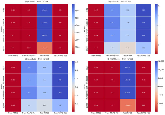
Figure 16.
Heatmap comparison of predictive model performance across variables for training and validation phases, using RMSE and MAPE as evaluation metrics: (a) General, (b) Latitude, (c) Longitude, and (d) Flight Level. Results are shown for KNN, XGBoost, Random Forest, and LSTM models.
In the General case Figure 16a, the conventional models show RMSE values around 6900 and MAPEs between 5.7% and 7%, underscoring their limited ability to capture broad spatiotemporal dynamics. By contrast, the LSTM model markedly reduces the error, achieving an RMSE of 1187 and a MAPE below 1%, thus demonstrating its superior capacity to represent global air traffic patterns. For Latitude Figure 16b, the differences among models are less pronounced due to the lower variability of this dimension. Even so, LSTM yields the lowest RMSE (2.49) and a MAPE of 3.58%, indicating better generalization to small-scale variations when compared with the other algorithms. The Longitude results Figure 16c follow a similar pattern. KNN, XGBoost, and Random Forest exhibit nearly identical performance (RMSE ≈ 2.09; MAPE ≈ 3%), whereas LSTM provides further improvements, with a RMSE of 1.65 and a MAPE of 2.21%.
These results highlight the recurrent model’s ability to consistently reduce residual errors in horizontal trajectory prediction. The most critical differences appear in Flight Level Figure 16d. Traditional approaches yield very high errors (RMSE ~12,000; MAPE > 30%), revealing their inability to adequately model vertical airspace dynamics. In stark contrast, LSTM achieves an RMSE close to 2020 and a MAPE of just 3.26%, evidencing its strength in capturing the nonlinear and sequential dependencies that govern vertical motion. Taken together, Figure 16 confirms that while conventional models may provide acceptable approximations for horizontal dimensions, they fail to generalize effectively in global and vertical contexts. LSTM consistently delivers substantially lower error magnitudes and more accurate proportional predictions across training and validation, establishing it as the most reliable and generalizable model for three-dimensional airspace trajectory forecasting.
Figure 17 presents violin plots of the residual distributions for the models evaluated in predicting latitude, longitude, and flight level. Each panel displays the comparison between training and validation phases, allowing for a visual assessment of the error behavior across different variables and learning contexts.

Figure 17.
Violin plots of residual distributions for predictive models: (a) Latitude, (b) Longitude, and (c) Flight Level, comparing training and validation phases.
In the case of latitude (a) and longitude (b), the residuals of KNN, XGBoost, and Random Forest exhibit wider and more dispersed shapes, reflecting higher average errors and limited explanatory power. In contrast, the LSTM model produces narrower, symmetric distributions centered close to zero, consistent with its lower MAE and RMSE values.
These results suggest that LSTM not only reduces the magnitude of prediction errors but also enhances the stability of spatial coordinate estimation. For flight level (c), the differences among models are even more pronounced. While traditional models generate residuals with very broad dispersions, often extending over thousands of feet, the LSTM residuals remain tightly concentrated within a few hundred feet. This marked contrast confirms the capacity of LSTM to capture sequential dependencies and nonlinear patterns inherent in vertical dynamics, which are critical for trajectory-based operations and airspace management.
In addition to predictive accuracy, the evaluation of the implemented models also considered their computational cost and inference latency, given the practical relevance of these aspects in air traffic management applications. All experiments were executed in Google Colab Pro+ using an NVIDIA A100 GPU as the hardware accelerator, ensuring high computational throughput and consistent runtime conditions. The dataset processed was approximately 800 MB in Parquet format (~61 million observations). Computational cost was estimated by measuring both training time and inference latency, using identical runtime configurations to ensure comparability across models.
The results presented in Table 4 highlight the differences in computational cost and latency among the evaluated models. KNN required virtually no training time but exhibited the highest inference latency, which is a direct consequence of its reliance on neighborhood searches across the full dataset. In contrast, Random Forest and XGBoost required several hours of training, with XGBoost showing the highest training overhead due to its iterative boosting process; however, both models achieved relatively low inference latency, making them suitable for near–real-time applications.

Table 4.
Computational cost and inference latency of the implemented models (KNN, Random Forest, XGBoost, and LSTM). The values illustrate the trade-off between training time, inference efficiency, and resource consumption across the different algorithms.
The LSTM network demanded the longest training time, reflecting the complexity of its sequential architecture, yet benefited the most from GPU acceleration by providing the lowest latency during inference. Overall, the table underscores the trade-off between training cost and inference efficiency, which is a critical consideration when selecting models for real-time airspace prediction tasks.
4. Discussion
The results obtained in this research are consistent with previous findings that highlight the effectiveness of LSTM neural networks in problems related to air trajectory prediction. In recent studies, the LSTM model has been recognized for its ability to capture complex temporal patterns, outperforming traditional models such as Random Forest, KNN, and XGBoost in similar tasks [13,59,60,61]. This research confirms those assertions by demonstrating that the LSTM model achieved the best results in terms of accuracy and explanatory capacity in predicting airspace occupancy in Colombia.
In particular, the LSTM achieved a general MAE of 312.59 and an RMSE of 1187.43, reflecting a significant reduction in error compared to KNN, XGBoost, and Random Forest, whose errors remained above 3400 (MAE) and 6800 (RMSE). Furthermore, the general coefficient of determination (R2 = 0.7523) positions LSTM as the only model capable of explaining more than 75% of the observed variability, which aligns with studies such as Zeng et al. [62] where LSTM was found to significantly outperform architectures like BP-NN or linear regression models in trajectory prediction tasks.
The precision of the LSTM model was also evident in the individual predictions of the three spatial dimensions. In latitude and longitude, absolute errors were lower than those reported in previous studies with conventional LSTM architectures, which documented average MAE values between 0.0095 and 0.0133 degrees [13,61]. Although this work did not incorporate hybrid models such as CNN-LSTM or BiLSTM-Attention—which have demonstrated additional improvements in spatial accuracy—the results of the proposed model are highly competitive. For example, the MAE of 1.7894 for latitude and 1.1042 for longitude reflects a robust capacity to model geographic patterns with good approximation, even without relying on attention mechanisms or convolutional layers.
The most notable difference achieved by the LSTM model was in the estimation of flight level, with an R2 of 0.9854, indicating an almost complete explanation of the vertical variability in air traffic. This result is particularly significant when compared with models such as CNN-LSTM or SS-DLSTM, which have been proposed to enhance prediction in complex scenarios such as terminal airspace [13,62]. While those architectures achieve high levels of precision in specific approach or departure points, the results presented in this study demonstrate that a standard LSTM model can achieve comparable levels of accuracy in more generalized prediction contexts.
Limitations of the Study
Despite the promising results obtained, this study presents several limitations that must be acknowledged. First, the analysis relied exclusively on ADS-B historical data from the Flightradar24 platform. While this source provides high-resolution information on aircraft trajectories, it does not incorporate other external factors that significantly influence air traffic dynamics, such as weather conditions, aircraft performance parameters, or airport operational restrictions.
The absence of these variables may limit the generalization of the results, particularly in scenarios characterized by high meteorological variability or atypical operational conditions. Additionally, data availability represents another constraint, as access to ADS-B records through Flightradar24 depends on commercial licensing. This may limit reproducibility and the possibility of extending the study to broader datasets without institutional agreements.
Second, the scope of the study was restricted to Colombian airspace. Although this provided a complex and heterogeneous environment for model validation, the findings cannot be directly extrapolated to other regions without additional testing. Airspaces with different traffic densities, regulatory frameworks, or infrastructural capacities may present challenges not addressed in this research.
Finally, the best-performing model (LSTM) required significant computational resources and long training times. This limitation may hinder its deployment in real-time systems or environments with constrained hardware capacity.
5. Conclusions
This study addressed the challenge of predicting Colombian airspace occupancy in 3D by applying machine learning algorithms to historical surveillance data. Using information collected through the ADS-B system, a predictive framework was developed to estimate future aircraft positions in terms of latitude, longitude, and flight level. The model was designed to support airspace planning and strategic decision-making processes, in alignment with the principles of Trajectory-Based Operations.
Among the algorithms evaluated—K-Nearest Neighbors, XGBoost, Random Forest, and Long Short-Term Memory networks—the LSTM model demonstrated the highest performance across all key metrics. With a Mean Absolute Error of 312.59, a Root Mean Squared Error of 1187.43, and a Coefficient of Determination of 0.7523, the LSTM model significantly outperformed traditional approaches. These results reflect its capacity to capture temporal dependencies within flight sequences and to deliver accurate predictions under complex and variable operational conditions.
The model’s ability to estimate flight level was particularly noteworthy, achieving an R2 of 0.9854, which indicates that it accounted for nearly all of the vertical variability observed in the dataset. In terms of spatial prediction, the LSTM also performed with high accuracy, producing significantly lower errors than the baseline models. These findings confirm its suitability for applications that demand robust, multivariable sequential prediction.
From a methodological perspective, one of the main contributions of this work lies in the adoption of a fully 3D approach to airspace occupancy prediction. This perspective goes beyond previous studies that have focused on individual trajectory points, offering a more comprehensive view of air traffic as a dynamic volume within the airspace.
Furthermore, the study demonstrated that reliable and precise predictions can be achieved through the exclusive use of historical data, without requiring additional external variables or overly complex modeling strategies. This enhances the scalability and real-world applicability of the proposed system.
6. Future Work
Future research may build upon the current findings in several directions. The integration of hybrid neural network architectures, such as CNN-LSTM or BiLSTM models enhanced with attention mechanisms, could improve both spatial accuracy and the modeling of complex temporal dependencies. Such approaches have shown potential in capturing nonlinear patterns and long-term dynamics, which are critical in high-dimensional trajectory prediction.
In addition, the development of real-time systems capable of embedding predictive outputs into visualization and monitoring tools would facilitate the direct application of these models in decision-support platforms for airspace management. Furthermore, linking predictive models with dynamic separation strategies and advanced planning mechanisms under the TBO framework could promote a more proactive and strategic approach to air traffic control.
Finally, research should also explore optimized or hybrid architectures that balance predictive accuracy with computational efficiency, as well as strategies for integrating multimodal datasets, including weather data, performance indicators, and airport operations, and expanding the analysis to multi-regional contexts. These directions would enhance the generalizability, practicality, and operational impact of predictive air traffic management systems.
Author Contributions
Conceptualization, J.O.R. and C.L.T.; methodology, J.O.R.; software, J.A.B.; validation, J.A.B. and P.M.D.; formal analysis, C.L.T.; investigation, I.R.B.; resources, C.L.T.; data curation, P.M.D.; writing—original draft preparation, I.R.B.; writing—review and editing, D.S.T.; visualization, D.S.T.; supervision, C.L.T.; project administration, C.L.T. All authors have read and agreed to the published version of the manuscript.
Funding
This research was funded by Fundación Universitaria Los Libertadores, grant number ING-47-25.
Data Availability Statement
The datasets presented in this article are not publicly available, as they were obtained from a private company. Requests for access should be directed to Cristian Lozano Tafur via the correspondence email.
Conflicts of Interest
The authors declare no conflicts of interest.
Abbreviations
The following abbreviations are used in this manuscript:
| 2D | Two-Dimensional |
| 3D | Three-Dimensional |
| 4D | Fourth Dimension |
| ADS -B | Automatic Dependent Surveillance-Broadcast |
| AI | Artificial Intelligence |
| AIP | Aeronautical Information Publication |
| ANN | Artificial Neural Network |
| ANSP | Air Navigation Service Providers |
| BLSTM | Bidirectional LSTM |
| CNN | Convolutional Neural Network |
| CRISP-DM | Cross-Industry Standard Process for Data Mining |
| DR | Discrepancy Ratio |
| DSR | Design Science Research |
| ELM | Extreme Learning Machines |
| FN | False Negatives |
| FP | False Positives |
| FRA | Free Route Airspace |
| FT | Feet |
| GANP | Global Air Navigation Plan |
| GNSS | Global Navigation Satellite Systems |
| HMM | Hidden Markov Models |
| ICAO | International Civil Aviation Organization |
| KNN | K-Nearest Neighbors |
| LGMB | Light Gradient Boosting Machine |
| LSTM | Long Short-Term Memory |
| MAE | Mean Absolute Error |
| MAPE | Mean Absolute Percentage Error |
| ML | Machine Learning |
| MLP | Multilayer Perceptron |
| MSE | Mean Squared Error |
| PCA | Principal Component Analysis |
| PSO | Particle Swarm Optimization |
| R | Pearson Correlation Coefficient |
| RMSE | Root Mean Squared Error |
| RNAV | Area Navigation |
| RNP | Required Navigation Performance |
| SI | Scatter Index |
| SVM | Support Vector Machines |
| TBO | Trajectory-Based Operations |
| TN | True Negatives |
| TP | True Positives |
| XGBoost | Extreme Gradient Boosting |
References
- ICAO. Future of Aviation; ICAO: Montreal, QC, Canada, 2019. [Google Scholar]
- ICAO. Plan Mundial de Navegación Aérea 2013–2028. In Capacidad y Eficiencia, 4th ed.; ICAO: Montreal, QC, Canada, 2013; pp. 8–30. [Google Scholar]
- Lutte, B. ICAO aviation system block upgrades: A method for identifying training needs. Int. J. Aviat. Aeronaut. Aerosp. 2015, 2, 2–16. [Google Scholar] [CrossRef]
- Aerocivil. AIP. Available online: https://www.aerocivil.gov.co/proveedor_servicios/publicaciones/3572/aip-publicacion-de-informacion-aeronautica (accessed on 20 March 2025).
- Aerocivil. RAC 91—Reglas Generales de Vuelo y de Operación; Aerocivil: Bogota, Colombia, 2024. [Google Scholar]
- Simões-Spencer, K. Fuel Consumption Optimization using Neural Networks and Genetic Algorithms. Master’s Thesis, Universidade Tecnica de Lisboa, Lisbon, Portugal, 2011. [Google Scholar]
- Medeiros, D.M.C.; Silva, J.M.R.; Bousson, K. RNAV and RNP AR approach systems: The case for Pico Island airport. Int. J. Aviat. Manag. 2012, 1, 181. [Google Scholar] [CrossRef]
- SESAR. SESAR Joint Undertaking|Background on Single European Sky. Available online: https://www.sesarju.eu/ (accessed on 11 May 2022).
- FAA. Next Generation Air Transportation System (NextGen); Federal Aviation Administration: Washington, DC, USA, 2015; pp. 28–30. [Google Scholar]
- Eurocontrol. Free Route Airspace; Eurocontrol: Brussels, Belgium, 2023. [Google Scholar]
- SkyVector. Flight Planning/Aeronautical Charts, SkyVector. Available online: https://skyvector.com/ (accessed on 15 November 2024).
- Zhang, X.; Zhong, S.; Mahadevan, S. Airport surface movement prediction and safety assessment with spatial–temporal graph convolutional neural network. Transp. Res. Part. C Emerg. Technol. 2022, 144, 103873. [Google Scholar] [CrossRef]
- Ma, L.; Tian, S. A Hybrid CNN-LSTM Model for Aircraft 4D Trajectory Prediction. IEEE Access 2020, 8, 134668–134680. [Google Scholar] [CrossRef]
- Ayhan, S.; Samet, H. Aircraft trajectory prediction made easy with predictive analytics. In Proceedings of the ACM SIGKDD International Conference on Knowledge Discovery and Data Mining, Association for Computing Machinery, San Francisco, CA, USA, 13–17 August 2016; pp. 21–30. [Google Scholar] [CrossRef]
- Tran, N.; Nguyen, H.Q.V.; Pham, D.T.; Alam, S. Aircraft Trajectory Prediction with Enriched Intent Using Encoder-Decoder Architecture. IEEE Access 2022, 10, 17881–17896. [Google Scholar] [CrossRef]
- Guan, X.; Lv, R.; Sun, L.; Liu, Y. A study of 4D trajectory prediction based on machine deep learning. In Proceedings of the World Congress on Intelligent Control and Automation (WCICA), Guilin, China, 12–17 June 2016; pp. 24–27. [Google Scholar] [CrossRef]
- Olive, X.; Basora, L. Detection and identification of significant events in historical aircraft trajectory data. Transp. Res. Part. C Emerg. Technol. 2020, 119, 102737. [Google Scholar] [CrossRef]
- Gil, D.; Hernandez-Sabate, A.; Enconniere, J.; Asmayawati, S.; Folch, P.; Borrego-Carazo, J.; Piera, M.À. E-Pilots: A System to Predict Hard Landing during the Approach Phase of Commercial Flights. IEEE Access 2022, 10, 7489–7503. [Google Scholar] [CrossRef]
- Alligier, R.; Gianazza, D.; Durand, N. Machine Learning Applied to Airspeed Prediction During Climb. IEEE Access 2021, 10, 7489–7503. [Google Scholar]
- Alligier, R.; Gianazza, D. Learning aircraft operational factors to improve aircraft climb prediction: A large scale multi-airport study. Transp. Res. Part. C Emerg. Technol. 2018, 96, 72–95. [Google Scholar] [CrossRef]
- Alligier, R. Predictive joint distribution of the mass and speed profile to improve aircraft climb prediction. In Proceedings of the 2020 International Conference on Artificial Intelligence and Data Analytics for Air Transportation, AIDA-AT 2020, Singapore, 3–4 February 2020. [Google Scholar] [CrossRef]
- Tong, C.; Yin, X.; Wang, S.; Zheng, Z. A novel deep learning method for aircraft landing speed prediction based on cloud-based sensor data. Future Gener. Comput. Syst. 2018, 88, 552–558. [Google Scholar] [CrossRef]
- Liu, X.; Huang, Y.; Wang, Q.; Song, Q.; Zhao, L. A prediction method for deck-motion of air-carrier based on PSO-KELM. In Proceedings of the International Conference on Sensing Technology, ICST, Nanjing, China, 11–13 November 2016. [Google Scholar] [CrossRef]
- Reitmann, S.; Nachtigall, K. Applying Bidirectional Long Short-Term Memories (BLSTM) to Performance Data in Air Traffic Management for System Identification; Lecture Notes in Computer Science (including subseries Lecture Notes in Artificial Intelligence and Lecture Notes in Bioinformatics); Springer: Berlin/Heidelberg, Germany, 2017; pp. 528–536. [Google Scholar] [CrossRef]
- Herrema, F.; Treve, V.; Desart, B.; Curran, R.; Visser, D. A novel machine learning model to predict abnormal Runway Occupancy Times and observe related precursors. In Proceedings of the 12th USA/Europe Air Traffic Management R and D Seminar, Seattle, WA, USA, 27–30 June 2017. [Google Scholar]
- Demir, E.; Demir, V.B. Predicting flight delays with artificial neural networks: Case study of an airport. In Proceedings of the 2017 25th Signal Processing and Communications Applications Conference (SIU), Antalya, Turkey, 15–18 May 2017; pp. 1–4. [Google Scholar] [CrossRef]
- Zhang, Q.; Mott, J.H.; Johnson, M.E.; Springer, J.A. Development of a Reliable Method for General Aviation Flight Phase Identification. IEEE Trans. Intell. Transp. Syst. 2022, 23, 11729–11738. [Google Scholar] [CrossRef]
- Ren, K.; Kim, A.M.; Kuhn, K. Exploration of the Evolution of Airport Ground Delay Programs. Transp. Res. Rec. 2018, 2672, 71–81. [Google Scholar] [CrossRef]
- Schröer, C.; Kruse, F.; Gómez, J.M. A systematic literature review on applying CRISP-DM process model. Procedia Comput. Sci. 2021, 181, 526–534. [Google Scholar] [CrossRef]
- Mtsweni, J.; Biermann, E.; Pretorius, L. iSemServ: A model-driven approach for developing semantic web services. S. Afr. Comput. J. 2014, 52, 55–70. [Google Scholar] [CrossRef]
- Zhang, J.; Liu, W.; Zhu, Y. Study of ADS-B data evaluation. Chin. J. Aeronaut. 2011, 24, 461–466. [Google Scholar] [CrossRef]
- García, S.; Luengo, J.; Herrera, F. Data Preprocessing in Data Mining. Intell. Syst. Ref. Libr. 2015, 72, 320. [Google Scholar]
- Ha, J.; Kambe, M.; Pe, J. Data Mining: Concepts and Techniques; Elsevier: Amsterdam, The Netherlands, 2011. [Google Scholar] [CrossRef]
- Jollife, I.T.; Cadima, J. Principal component analysis: A review and recent developments. R. Soc. Lond. 2016, 374, 20150202. [Google Scholar] [CrossRef] [PubMed]
- Kuhn, M.; Johnson, K. Applied Predictive Modeling; Springer: New York, NY, USA, 2013; pp. 1–600. [Google Scholar] [CrossRef]
- Seibold, H.; Hothorn, T.; Zeileis, A. Generalised linear model trees with global additive effects. Adv. Data Anal. Classif. 2019, 13, 703–725. [Google Scholar] [CrossRef]
- Ming, W.; Bao, Y.; Hu, Z.; Xiong, T. Multistep-Ahead Air Passengers Traffic Prediction with Hybrid ARIMA-SVMs Models. Sci. World J. 2014, 2014, 567246. [Google Scholar] [CrossRef]
- Guo, G.; Wang, H.; Bell, D.; Bi, Y.; Greer, K. KNN model-based approach in classification. In Lecture Notes in Computer Science (Including Subseries Lecture Notes in Artificial Intelligence and Lecture Notes in Bioinformatics), 2888; Springer: Berlin/Heidelberg, Germany, 2003; pp. 986–996. [Google Scholar] [CrossRef]
- Shai, S.-S.; Shai, B.-D. Understanding Machine Learning: From Theory to Algorithms; Cambridge University Press: Cambridge, UK, 2014. [Google Scholar]
- Gabrillia, C. Implementation of the K-Nearest Neighbor Algorithm to Predict Air Pollution. Inf. Technol. Syst. 2023, 1, 45–54. [Google Scholar] [CrossRef]
- Fredriksson, K. Geometric Near-Neighbor Access Tree (GNAT) Revisited, May 2016. Available online: https://arxiv.org/abs/1605.05944v2 (accessed on 24 February 2025).
- Espinosa, J. Aplicación de algoritmos Random Forest y XGBoost en una base de solicitudes de tarjetas de crédito. Ing. Investig. Tecnol. 2020, 21, 1–16. [Google Scholar] [CrossRef]
- Recarey, R. Métodos de Ensamblado en Machine Learning, Universidade de Santiago de Compostela, 2021. Available online: http://eio.usc.es/pub/mte/descargas/ProyectosFinMaster/Proyecto_1686.pdf (accessed on 24 February 2025).
- Midtfjord, A.D.; De Bin, R.; Huseby, A.B. A decision support system for safer airplane landings: Predicting runway conditions using XGBoost and explainable AI. Cold Reg. Sci. Technol. 2022, 199, 103556. [Google Scholar] [CrossRef]
- Shi, Z.; Xu, M.; Pan, Q.; Yan, B.; Zhang, H. LSTM-based Flight Trajectory Prediction. In Proceedings of the International Joint Conference on Neural Networks, Rio de Janeiro, Brazil, 8–13 July 2018. [Google Scholar] [CrossRef]
- Pang, Y.; Xu, N.; Liu, Y. Aircraft trajectory prediction using lstm neural network with embedded convolutional layer. In Proceedings of the Annual Conference of the Prognostics and Health Management Society, PHM, Prognostics and Health Management Society, Scottsdale, AZ, USA, 21–26 September 2019. [Google Scholar] [CrossRef]
- Breiman, L. Random forests. Mach. Learn. 2001, 45, 5–32. [Google Scholar] [CrossRef]
- Yan, B.; Zhang, X.; Tang, C.; Wang, X.; Yang, Y.; Xu, W. A Random Forest-Based Method for Predicting Borehole Trajectories. Mathematics 2023, 11, 1297. [Google Scholar] [CrossRef]
- Hashemi, S.M.; Botez, R.M.; Ghazi, G. Robust Trajectory Prediction Using Random Forest Methodology Application to UAS-S4 Ehécatl. Aerospace 2024, 11, 49. [Google Scholar] [CrossRef]
- Chai, T.; Draxler, R.R. Root mean square error (RMSE) or mean absolute error (MAE)?—Arguments against avoiding RMSE in the literature. Geosci. Model. Dev. 2014, 7, 1247–1250. [Google Scholar] [CrossRef]
- De Myttenaere, A.; Golden, B.; Le Grand, B.; Rossi, F. Mean Absolute Percentage Error for regression models. Neurocomputing 2016, 192, 38–48. [Google Scholar] [CrossRef]
- Hintze, J.L.; Nelson, R.D. Violin plots: A box plot-density trace synergism. Am. Stat. 1998, 52, 181–184. [Google Scholar] [CrossRef]
- Wang, Z.; Liang, M.; Delahaye, D. A hybrid machine learning model for short-term estimated time of arrival prediction in terminal manoeuvring area. Transp. Res. Part. C Emerg. Technol. 2018, 95, 280–294. [Google Scholar] [CrossRef]
- Mukaka, M.M. A guide to appropriate use of Correlation coefficient in medical research. Malawi Med. J. 2012, 24, 69. Available online: https://pmc.ncbi.nlm.nih.gov/articles/PMC3576830/ (accessed on 10 September 2025). [PubMed]
- Jolliff, J.K.; Kindle, J.C.; Shulman, I.; Penta, B.; Friedrichs, M.A.; Helber, R.; Arnone, R.A. Summary diagrams for coupled hydrodynamic-ecosystem model skill assessment. J. Mar. Syst. 2009, 76, 64–82. [Google Scholar] [CrossRef]
- Doerr, C.; Gnewuch, M.; Wahlström, M. Calculation of Discrepancy Measures and Applications. In A Panorama of Discrepancy Theory; Springer: Cham, Switzerland, 2014. [Google Scholar] [CrossRef]
- Plan, E.L. Modeling and simulation of count data. CPT Pharmacometrics Syst. Pharmacol. 2014, 3, 1–12. [Google Scholar] [CrossRef]
- Wilkinson, L.; Friendly, M. The History of the Cluster Heat Map. Am. Stat. 2009, 63, 179–184. [Google Scholar] [CrossRef]
- Schimpf, N.; Wang, Z.; Li, S.; Knoblock, E.J.; Li, H.; Apaza, R.D. A Generalized Approach to Aircraft Trajectory Prediction via Supervised Deep Learning. IEEE Access 2023, 11, 116183–116195. [Google Scholar] [CrossRef]
- Silvestre, J.; Mielgo, P.; Bregon, A.; Martinez-Prieto, M.A.; Alvarez-Esteban, C. Multi-route aircraft trajectory prediction using Temporal Fusion Transformers. IEEE Access 2024, 12, 174094–174106. [Google Scholar] [CrossRef]
- Wu, Y.; Yu, H.; Du, J.; Liu, B.; Yu, W. An Aircraft Trajectory Prediction Method Based on Trajectory Clustering and a Spatiotemporal Feature Network. Electronics 2022, 11, 3453. [Google Scholar] [CrossRef]
- Zeng, W.; Quan, Z.; Zhao, Z.; Xie, C.; Lu, X. A Deep Learning Approach for Aircraft Trajectory Prediction in Terminal Airspace. IEEE Access 2020, 8, 151250–151266. [Google Scholar] [CrossRef]
Disclaimer/Publisher’s Note: The statements, opinions and data contained in all publications are solely those of the individual author(s) and contributor(s) and not of MDPI and/or the editor(s). MDPI and/or the editor(s) disclaim responsibility for any injury to people or property resulting from any ideas, methods, instructions or products referred to in the content. |
© 2025 by the authors. Licensee MDPI, Basel, Switzerland. This article is an open access article distributed under the terms and conditions of the Creative Commons Attribution (CC BY) license (https://creativecommons.org/licenses/by/4.0/).