SGR-Net: A Synergistic Attention Network for Robust Stock Market Forecasting
Abstract
1. Introduction
1.1. Contributions
- Propose a novel Multi-Perspective Fused Attention model: We developed a Multi-Perspective Fused Attention-based deep learning model (SGR-Net) that amalgamates the strengths of different Fused Attention mechanisms to efficiently capture uncertain temporal dependencies in stock time-series data, interdependency among technical indicators, and intricate patterns in financial time-series data.
- Address key limitations of previous studies using attention-based models: Prior studies on stock market forecasting were based on individual attention approaches or standalone deep learning models. However, these models had difficulty focusing on time steps that have a significant influence on model predictions, were unable to capture long-term dependencies, and struggled to deal with noise in time-series sequences. In order to overcome these limitations, we adopted three complementary attention mechanisms: Sparse Attention, which focuses on impactful time steps while simultaneously reducing computation time; Global Attention, which captures long-term dependencies in sequences; and Random Attention, which mitigates noise and reduces overfitting. We thus produced a model that is both robust and generalizable.
- Engineer a rich input feature space: The utilization of 13 technical indicators in this study enriched the feature space for model learning, thereby enabling the proposed Fused Attention model to learn intricate patterns and capture trends in stock indices efficiently.
- Conduct extensive empirical analysis across nine global stock indices: Assessed the model’s performance on nine volatile global stock market indices, validating its performance and adaptability across a range of financial tasks.
- Demonstrate superior performance and efficiency: We evaluated multiple global stock indices to showcase the noteworthiness of the proposed Fused Attention model, which not only maintains computational efficiency but also generalizes well across varied market conditions.
1.2. Organization
2. Related Work
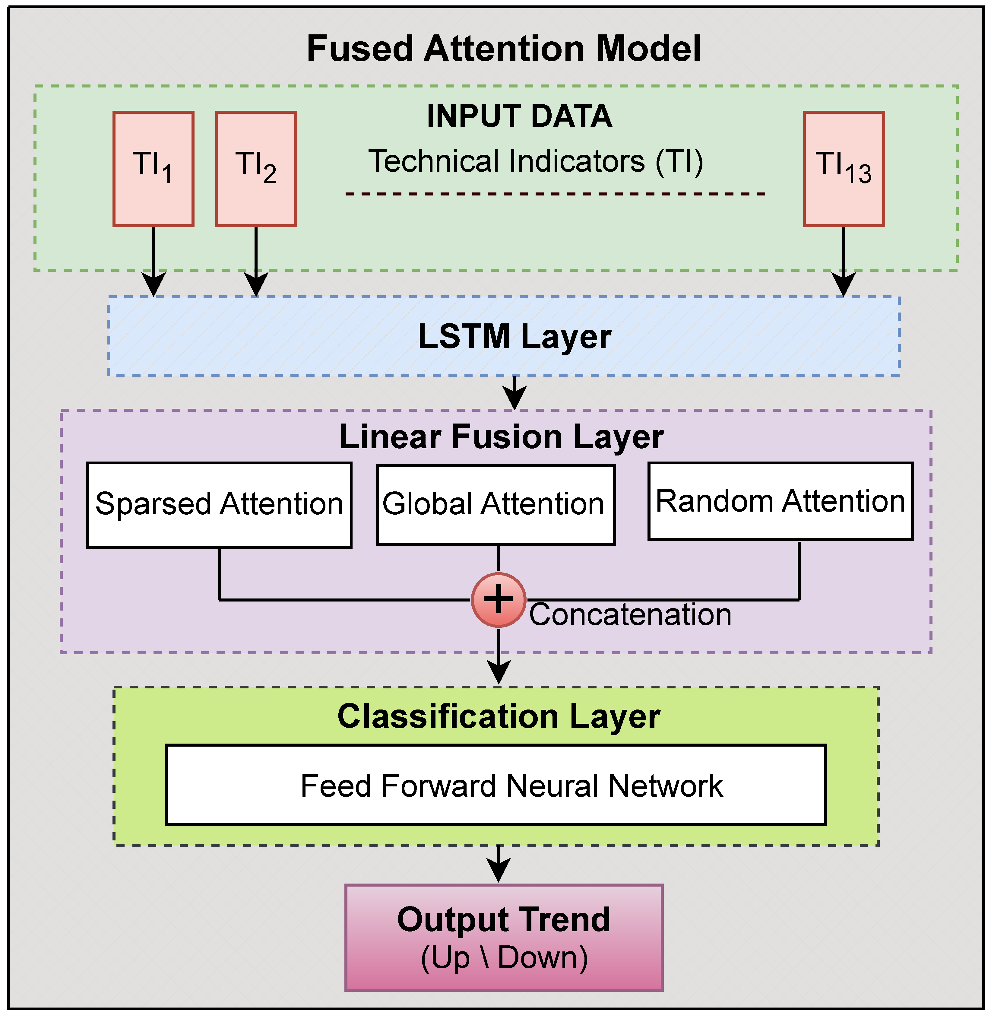
3. Propose Model Architecture
- Input Layer: It process several technical indicators derived from past raw stock market data as inputs.
- LSTM Layer: It captures the sequential dependencies in the financial time-series data.
- Sparse Attention Module: It focuses on important, significant time steps under a sparsity restriction.
- Global Attention Module: It assigns dynamic priority values across all time steps.
- Random Attention Module: It provides random weight assignment meant to enhance generalization.
- Fusion Layer: The fusion layer combines attention outputs with feature representation improvement.
- Feedforward Network: The feedforward network classifies final stock market trends as up/down.
3.1. Input Layer
- X is the input data with the shape (batch_size, seq_len, input_size).
- Each represents a feature vector that includes 13 technical indicators at time step t.
3.2. LSTM Layer
- Forget Gate (Filtering Old Information):
- Input Gate (Deciding What to Store):
- Candidate Memory Update (New-Information Processing):
- Memory Cell Update (Retaining Important Information):
- Output Gate (Deciding What to Reveal as Output):
- Final Hidden State Calculation:
- The forget, input, and output gates are denoted by , and .
- The sigmoid activation function is denoted by .
- The cell state capturing memory across time steps is denoted by .
- The forget gate weights are denoted by and .
- The input gate weights are denoted by and .
- The memory update weights are denoted by and .
- The output gate weights are denoted by and .
- Biases are denoted by .
3.3. Attention Mechanisms
3.3.1. Sparse Attention
- is a learned parameter.
- denotes the Sparse Attention context vector.
3.3.2. Global Attention
- is a trainable parameter.
- denotes the Global Attention context vector.
3.3.3. Random Attention
- is a uniform random distribution.
- denotes the Random Attention context vector.
3.4. Fusion Layer
- is a learnable weight matrix.
- is a bias term.
3.5. Feedforward Network
- First Layer:
- –
- This layer consists of a fully connected layer.
- –
- The activation function used in this layer is .
- Second Layer:
- –
- This is a fully connected layer.
- –
- The activation function used in this layer is the sigmoid activation function, for predicting uptrends and downtrends.
The final prediction is calculated asfor binary classification.
4. Dataset Description
- Bombay Stock Exchange, India’s BSE index.
- Germany’s DAX index, Deutscher Aktienindex.
- Dow Jones Industrial Average, USA (DJUS).
- NASDAQ—USA’s Composite Index.
- NIFTY 50: National Stock Exchange of India.
- Nikkei 225 Tokyo Stock Exchange, Japan.
- NYSE AMEX: NYSE American Composite Index, USA.
- Standard and Poor’s 500, USA (S&P 500).
- Shanghai stock index—China’s Shanghai Stock Exchange.
4.1. Preprocessing and Data Collection
4.2. Feature Engineering
- Simple Moving Average (ten-day SMA);
- Ten-day Weighted Moving Average (WMA);
- Stochastic %K (fourteen-day indicator);
- Stochastic %D (three-day moving average of %K);
- Five-day Discrepancy Index;
- Ten-day Disparity Index;
- Ten-day Oscillator Percentage (OSCP);
- Ten-day Momentum;
- Relative Strength Index (RSI; fourteen-day index);
- Larry Williams %R (fourteen-day indicator);
- Accumulation and Distribution Indicator (A/D);
- Twenty-day Commodity Channel Index (CCI);
- Moving Average Convergence Divergence (MACD: 12, 26, 9).
- It takes a value of 1 (up) when the closing price of the next day surpasses that of the current day.
- It takes a value of 0 (down) when the closing price of the next day is lower than that of the current day.
4.3. Dataset Details
5. Experimental Setup
6. Result Analysis and Discussion
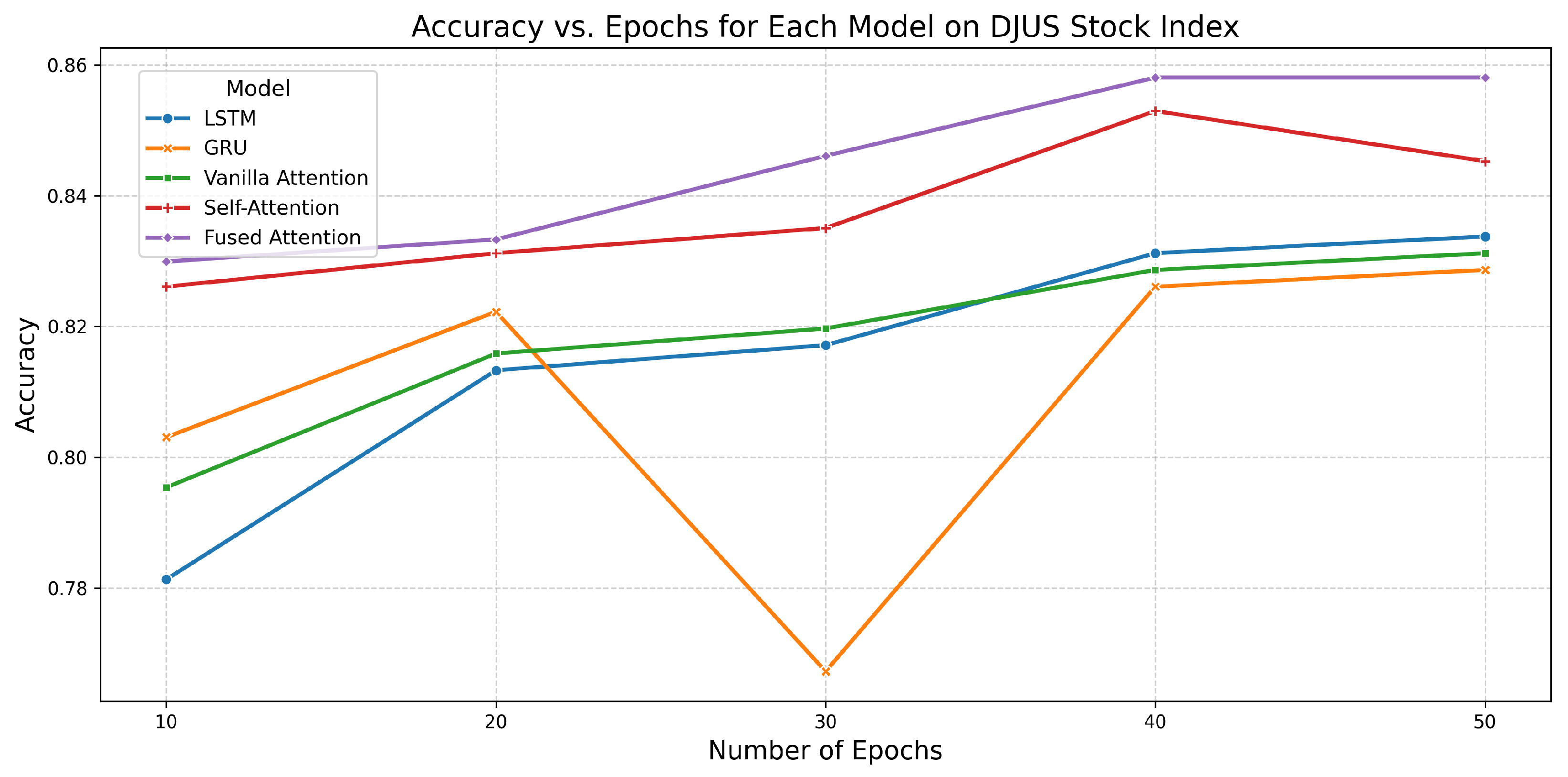
6.1. Performance of All Models on DJUS Stock Index
| Model | Epochs | Accuracy | AUC | Training Time (s) |
|---|---|---|---|---|
| LSTM | 10 | 0.7813 | 0.8869 | 1.4998 |
| 20 | 0.8133 | 0.9020 | 2.3865 | |
| 30 | 0.8171 | 0.9077 | 4.2865 | |
| 40 | 0.8312 | 0.9130 | 4.8311 | |
| 50 | 0.8338 | 0.9164 | 6.6354 | |
| GRU | 10 | 0.8031 | 0.8870 | 1.0240 |
| 20 | 0.8223 | 0.9019 | 2.2396 | |
| 30 | 0.7673 | 0.9063 | 3.3364 | |
| 40 | 0.8261 | 0.9127 | 4.0333 | |
| 50 | 0.8286 | 0.9170 | 5.7167 | |
| Vanilla Attention | 10 | 0.7954 | 0.8845 | 1.5839 |
| 20 | 0.8159 | 0.9016 | 2.6829 | |
| 30 | 0.8197 | 0.9080 | 4.1972 | |
| 40 | 0.8286 | 0.9124 | 6.1048 | |
| 50 | 0.8312 | 0.9162 | 6.7852 | |
| Self-Attention | 10 | 0.8261 | 0.9101 | 1.9021 |
| 20 | 0.8312 | 0.9180 | 4.4426 | |
| 30 | 0.8350 | 0.9260 | 6.0507 | |
| 40 | 0.8529 | 0.9318 | 8.1773 | |
| 50 | 0.8453 | 0.9393 | 10.1723 | |
| Fused Attention | 10 | 0.8299 | 0.9144 | 2.5265 |
| 20 | 0.8333 | 0.9265 | 4.1947 | |
| 30 | 0.8461 | 0.9345 | 6.7247 | |
| 40 | 0.8581 | 0.9401 | 8.1700 | |
| 50 | 0.8581 | 0.9442 | 10.9043 |

6.2. Performance of All Models on NYSE AMEX Stock Index
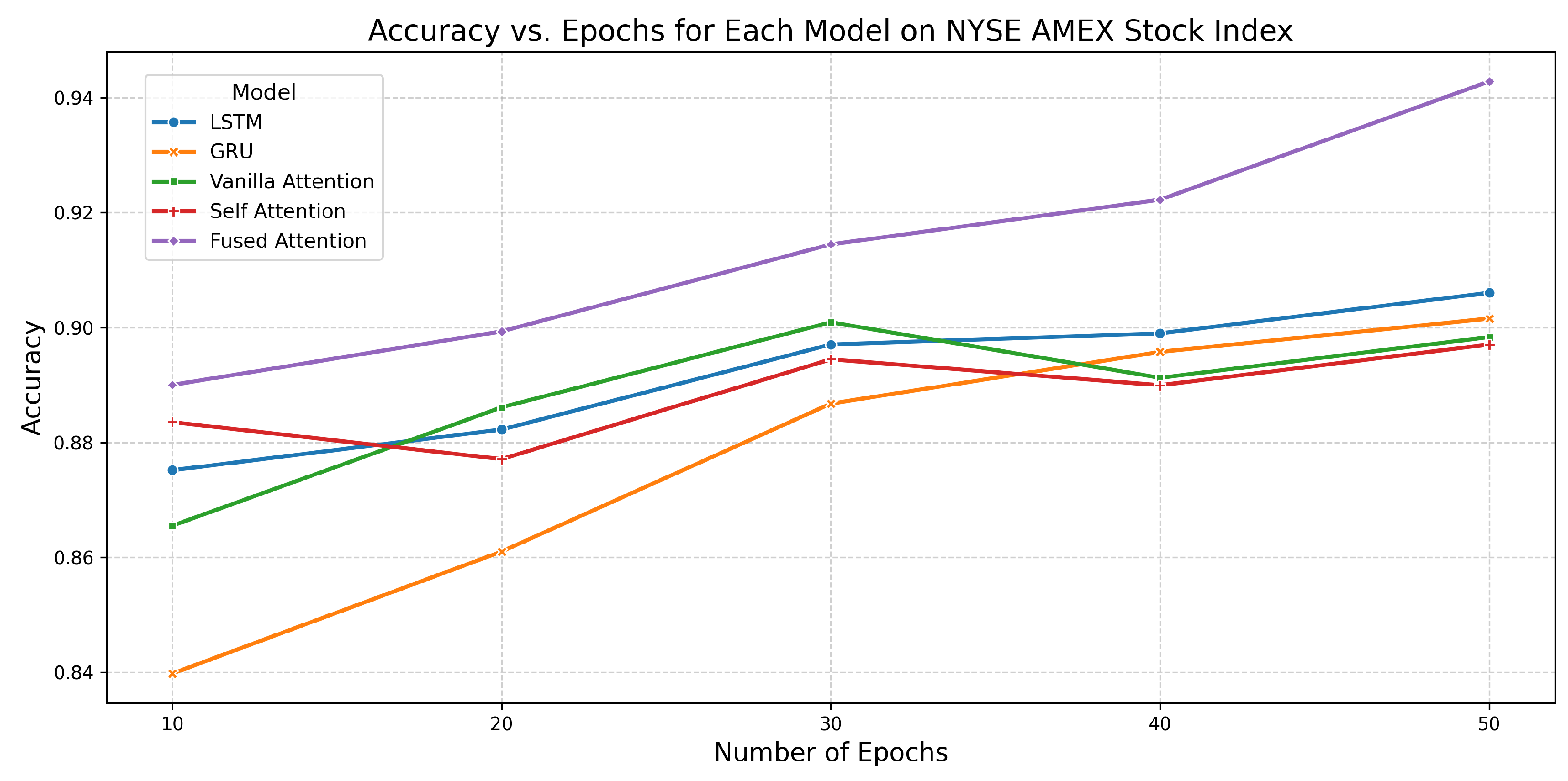
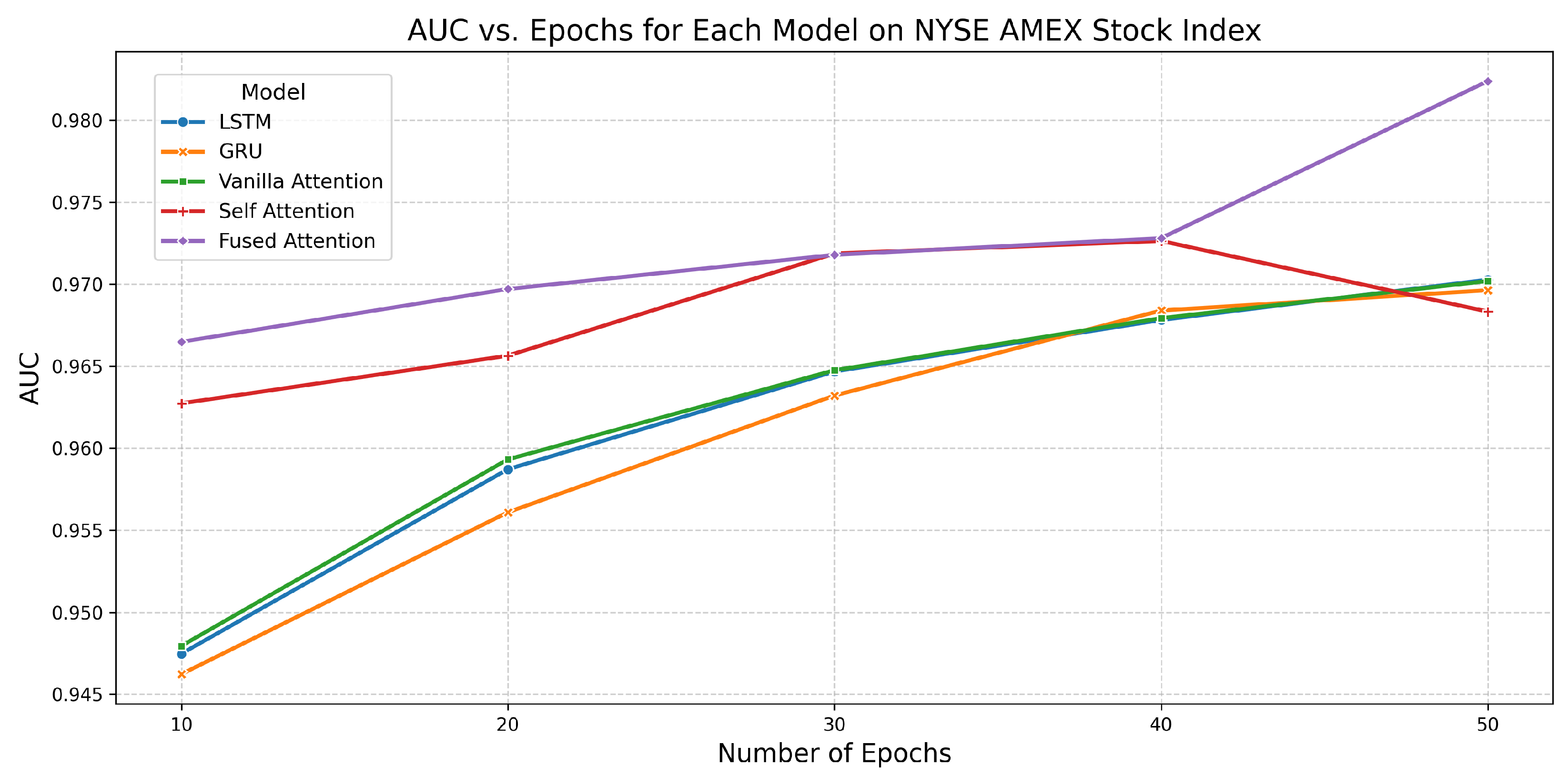
| Model | Epochs | Accuracy | AUC | Training Time (s) |
|---|---|---|---|---|
| LSTM | 10 | 0.8752 | 0.9475 | 2.9539 |
| 20 | 0.8822 | 0.9587 | 6.0131 | |
| 30 | 0.8970 | 0.9647 | 8.3584 | |
| 40 | 0.8990 | 0.9678 | 10.2014 | |
| 50 | 0.9060 | 0.9703 | 14.3584 | |
| GRU | 10 | 0.8398 | 0.9462 | 2.2718 |
| 20 | 0.8610 | 0.9561 | 4.2328 | |
| 30 | 0.8867 | 0.9632 | 7.2727 | |
| 40 | 0.8958 | 0.9684 | 9.0038 | |
| 50 | 0.9015 | 0.9696 | 10.0793 | |
| Vanilla Attention | 10 | 0.8655 | 0.9479 | 3.1822 |
| 20 | 0.8861 | 0.9593 | 5.4869 | |
| 30 | 0.9009 | 0.9648 | 9.4229 | |
| 40 | 0.8912 | 0.9679 | 13.1927 | |
| 50 | 0.8983 | 0.9702 | 18.9116 | |
| Self-Attention | 10 | 0.8835 | 0.9627 | 4.4814 |
| 20 | 0.8771 | 0.9656 | 9.0363 | |
| 30 | 0.8945 | 0.9719 | 12.1958 | |
| 40 | 0.8900 | 0.9726 | 16.4426 | |
| 50 | 0.8970 | 0.9683 | 21.4925 | |
| Fused Attention | 10 | 0.8900 | 0.9665 | 5.2198 |
| 20 | 0.8993 | 0.9697 | 8.7127 | |
| 30 | 0.9145 | 0.9718 | 13.9070 | |
| 40 | 0.9222 | 0.9728 | 17.9407 | |
| 50 | 0.9428 | 0.9824 | 22.6548 |
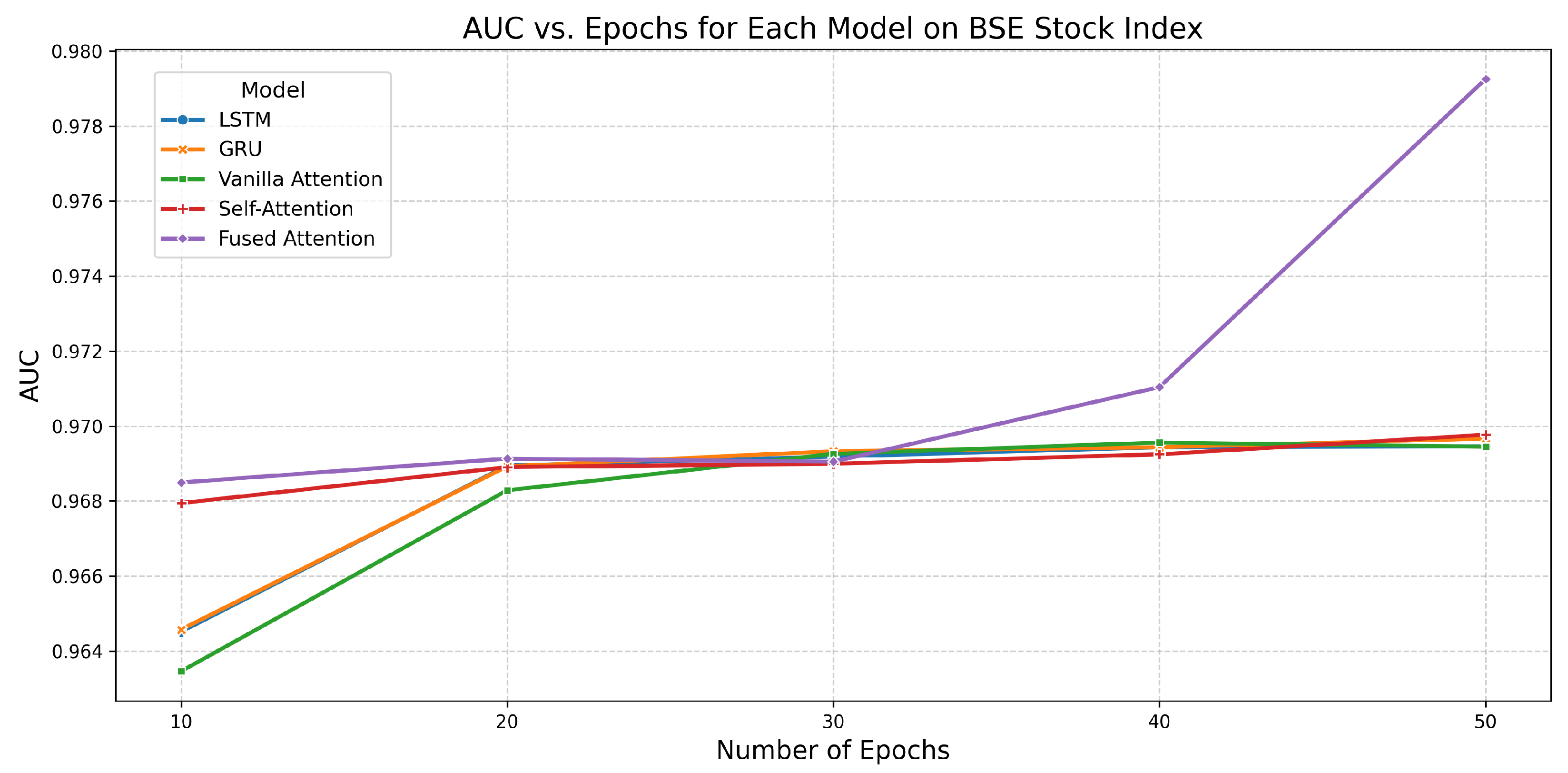
6.3. Performance of All Models on BSE Stock Index
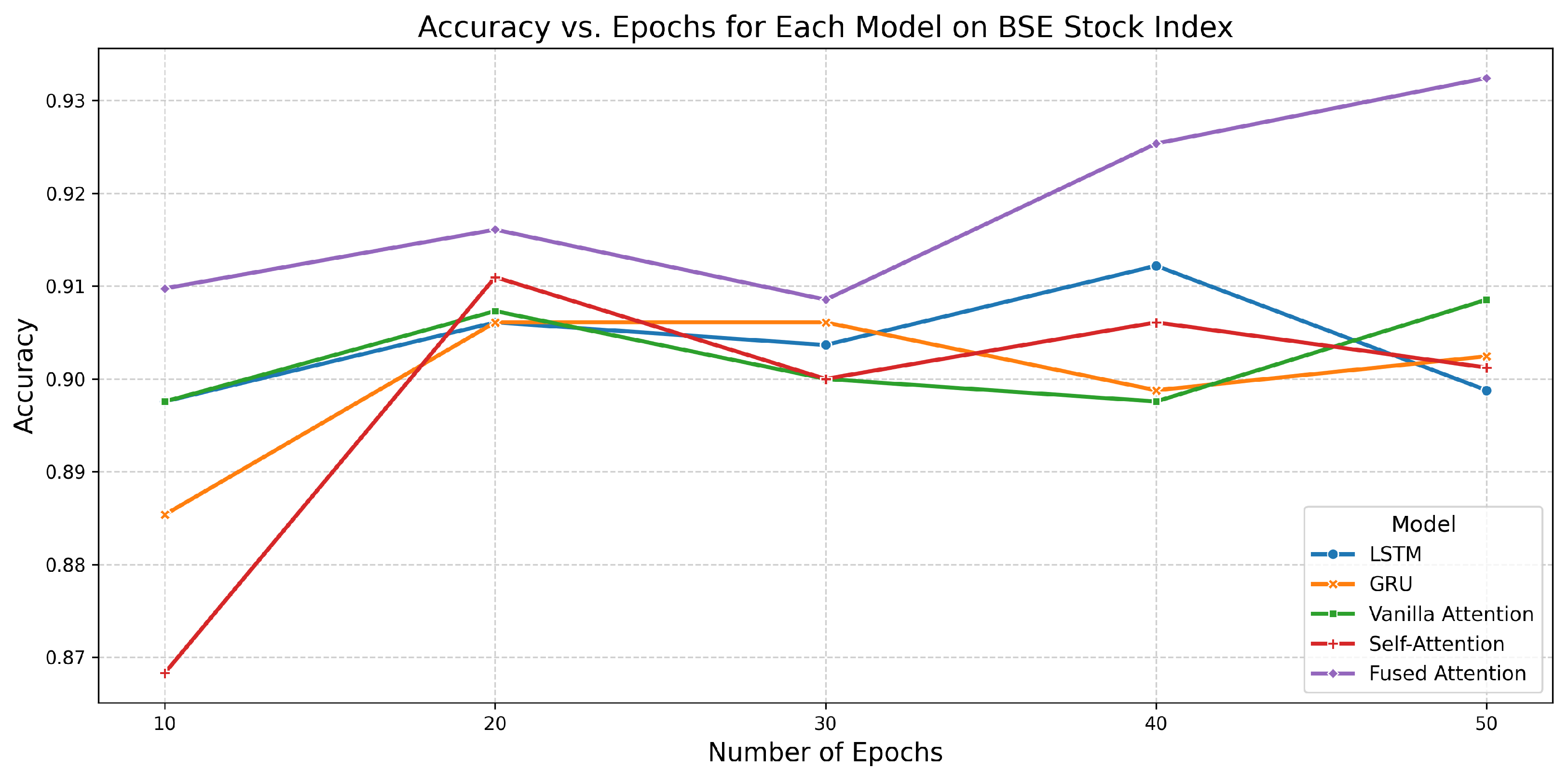
| Model | Epochs | Accuracy | AUC | Training Time (s) |
|---|---|---|---|---|
| LSTM | 10 | 0.8976 | 0.9645 | 3.3735 |
| 20 | 0.9061 | 0.9689 | 6.8165 | |
| 30 | 0.9037 | 0.9692 | 12.2368 | |
| 40 | 0.9122 | 0.9694 | 12.4857 | |
| 50 | 0.8988 | 0.9695 | 15.2494 | |
| GRU | 10 | 0.8854 | 0.9646 | 2.2977 |
| 20 | 0.9061 | 0.9689 | 5.4531 | |
| 30 | 0.9061 | 0.9693 | 7.0210 | |
| 40 | 0.8988 | 0.9694 | 10.3086 | |
| 50 | 0.9024 | 0.9697 | 12.0394 | |
| Vanilla Attention | 10 | 0.8976 | 0.9635 | 3.1332 |
| 20 | 0.9073 | 0.9683 | 7.9487 | |
| 30 | 0.9000 | 0.9693 | 10.4125 | |
| 40 | 0.8976 | 0.9696 | 13.8738 | |
| 50 | 0.9085 | 0.9694 | 16.2311 | |
| Self-Attention | 10 | 0.8683 | 0.9679 | 4.6417 |
| 20 | 0.9110 | 0.9689 | 7.7108 | |
| 30 | 0.9000 | 0.9690 | 13.3624 | |
| 40 | 0.9061 | 0.9692 | 18.6159 | |
| 50 | 0.9012 | 0.9698 | 21.5084 | |
| Fused Attention | 10 | 0.9098 | 0.9685 | 5.3015 |
| 20 | 0.9161 | 0.9691 | 9.1033 | |
| 30 | 0.9085 | 0.9690 | 14.7980 | |
| 40 | 0.9254 | 0.9710 | 19.3200 | |
| 50 | 0.9324 | 0.9793 | 21.9127 |
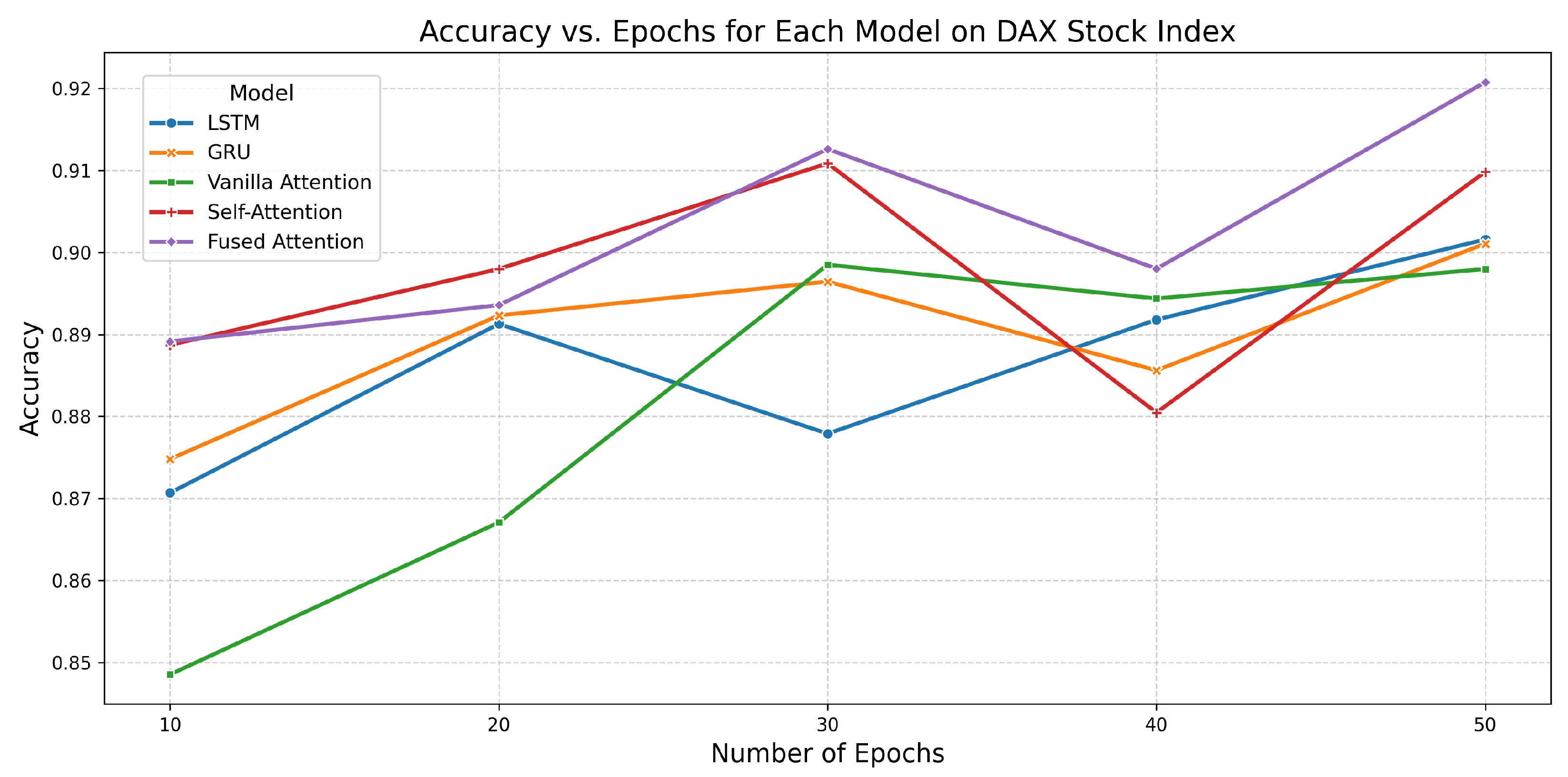
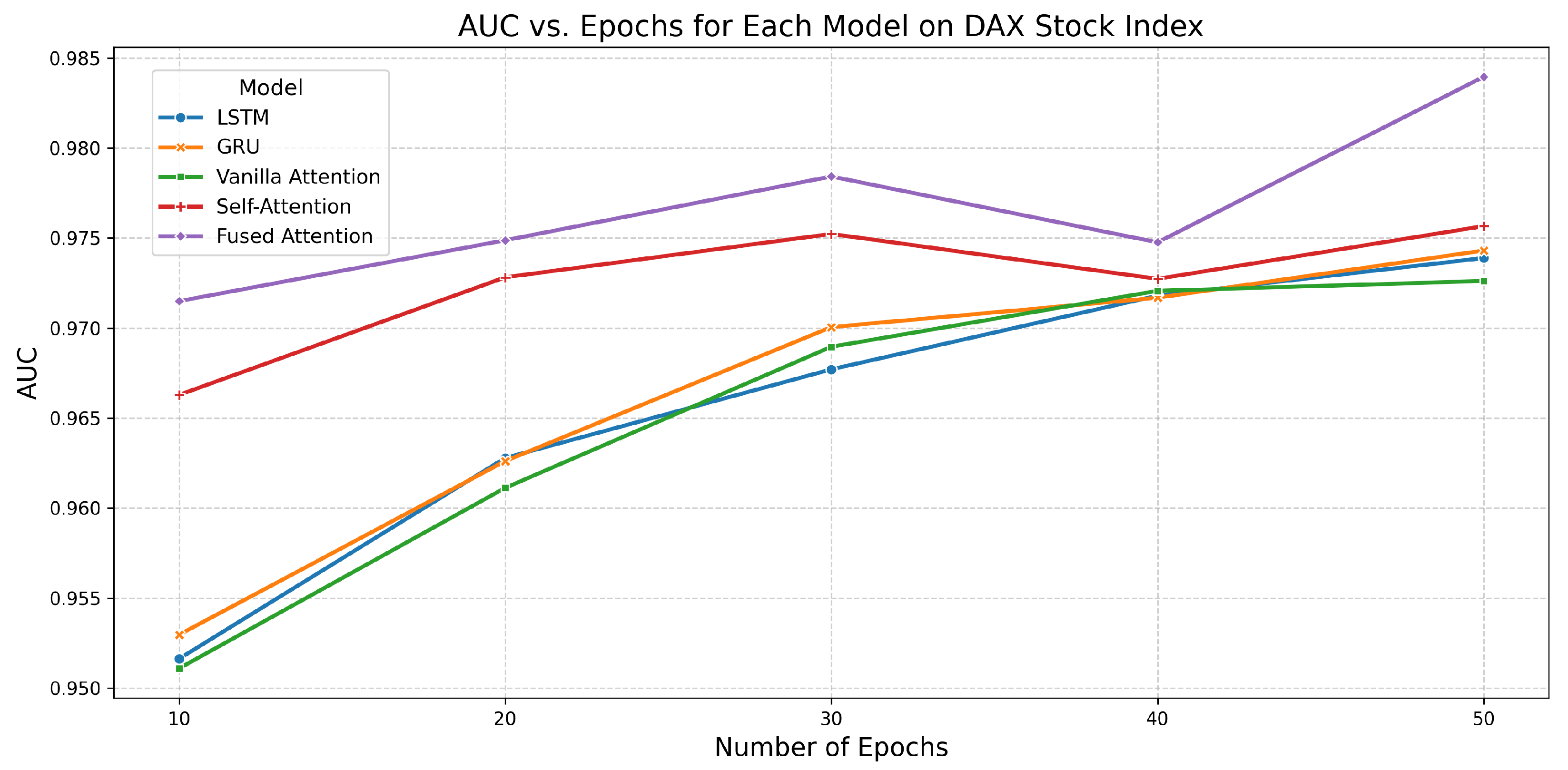
6.4. Performance of All Models on DAX Stock Index
| Model | Epochs | Accuracy | AUC | Training Time (s) |
|---|---|---|---|---|
| LSTM | 10 | 0.8707 | 0.9516 | 5.1605 |
| 20 | 0.8913 | 0.9628 | 11.9538 | |
| 30 | 0.8779 | 0.9677 | 17.2379 | |
| 40 | 0.8918 | 0.9718 | 21.3852 | |
| 50 | 0.9016 | 0.9739 | 27.1811 | |
| GRU | 10 | 0.8748 | 0.9530 | 5.9193 |
| 20 | 0.8923 | 0.9626 | 9.1716 | |
| 30 | 0.8964 | 0.9701 | 12.9187 | |
| 40 | 0.8856 | 0.9717 | 17.0575 | |
| 50 | 0.9011 | 0.9743 | 20.9216 | |
| Vanilla Attention | 10 | 0.8485 | 0.9511 | 11.0104 |
| 20 | 0.8671 | 0.9611 | 11.9999 | |
| 30 | 0.8985 | 0.9690 | 17.4971 | |
| 40 | 0.8944 | 0.9721 | 26.3364 | |
| 50 | 0.8980 | 0.9726 | 29.6048 | |
| Self-Attention | 10 | 0.8887 | 0.9663 | 9.0568 |
| 20 | 0.8980 | 0.9728 | 15.8787 | |
| 30 | 0.9109 | 0.9752 | 24.8836 | |
| 40 | 0.8805 | 0.9727 | 34.1670 | |
| 50 | 0.9098 | 0.9757 | 43.9295 | |
| Fused Attention | 10 | 0.8891 | 0.9715 | 10.0830 |
| 20 | 0.8936 | 0.9749 | 17.8837 | |
| 30 | 0.9126 | 0.9784 | 27.9773 | |
| 40 | 0.8980 | 0.9748 | 36.8110 | |
| 50 | 0.9208 | 0.9840 | 44.7582 |
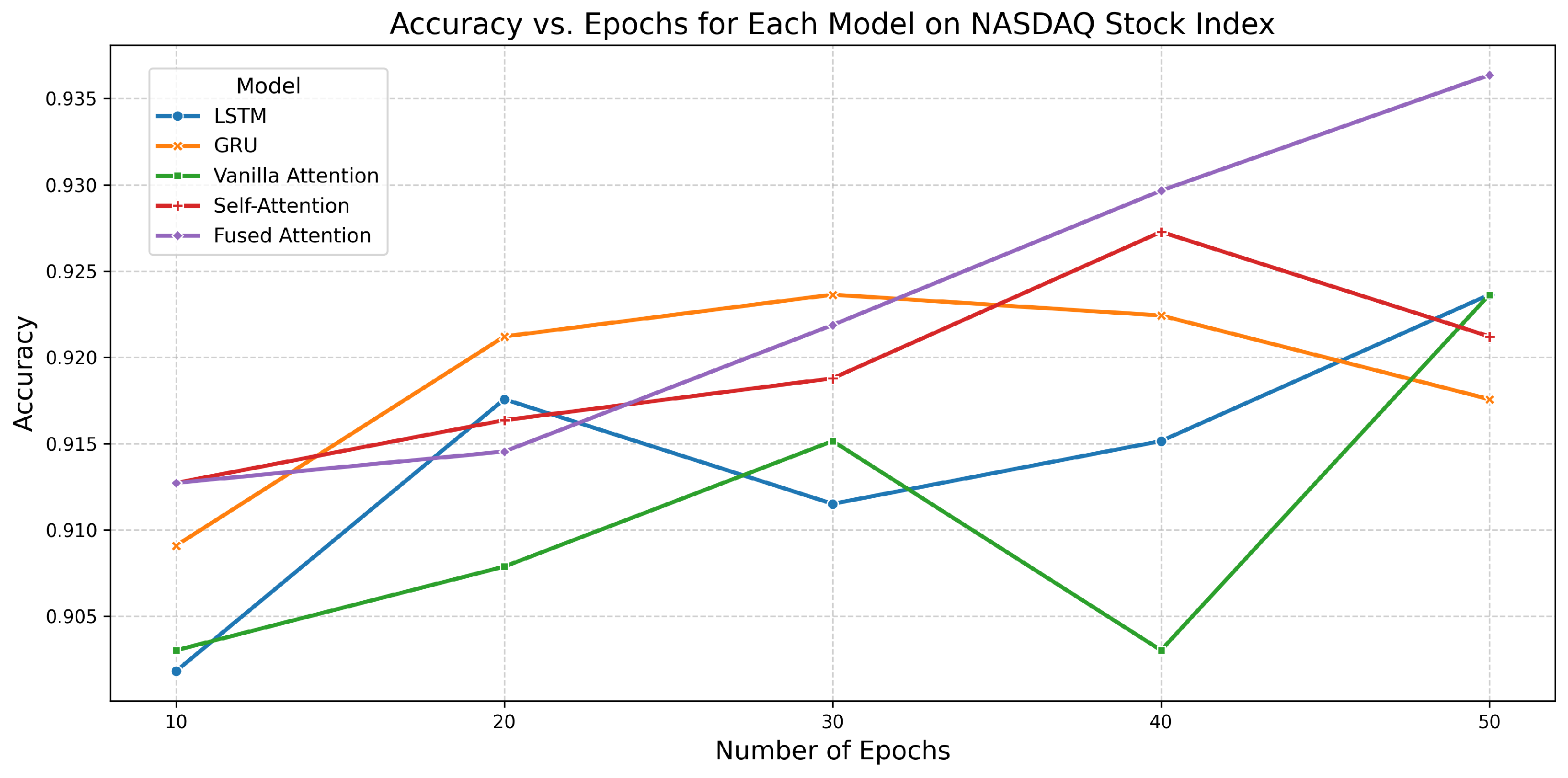
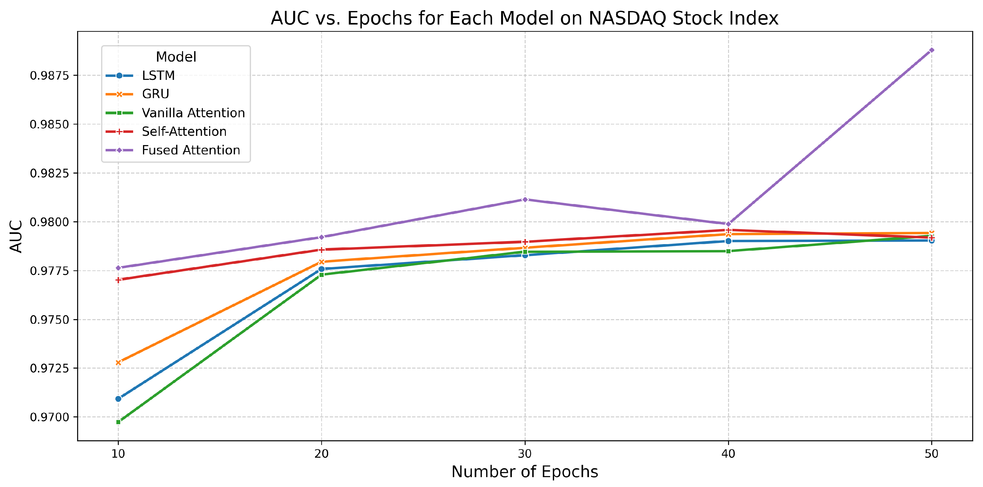
6.5. Performance of All Models on NASDAQ Stock Index
| Model | Epochs | Accuracy | AUC | Training Time (s) |
|---|---|---|---|---|
| LSTM | 10 | 0.9018 | 0.9709 | 5.9462 |
| 20 | 0.9176 | 0.9776 | 6.9876 | |
| 30 | 0.9115 | 0.9783 | 9.7193 | |
| 40 | 0.9152 | 0.9790 | 12.0025 | |
| 50 | 0.9236 | 0.9790 | 16.2997 | |
| GRU | 10 | 0.9091 | 0.9728 | 2.2077 |
| 20 | 0.9212 | 0.9779 | 4.4367 | |
| 30 | 0.9236 | 0.9787 | 7.6702 | |
| 40 | 0.9224 | 0.9794 | 8.3064 | |
| 50 | 0.9176 | 0.9794 | 11.8980 | |
| Vanilla Attention | 10 | 0.9030 | 0.9697 | 3.2347 |
| 20 | 0.9079 | 0.9773 | 6.9445 | |
| 30 | 0.9152 | 0.9785 | 10.4709 | |
| 40 | 0.9030 | 0.9785 | 12.8610 | |
| 50 | 0.9236 | 0.9793 | 15.8315 | |
| Self-Attention | 10 | 0.9127 | 0.9770 | 3.8595 |
| 20 | 0.9164 | 0.9786 | 9.8097 | |
| 30 | 0.9188 | 0.9790 | 12.5427 | |
| 40 | 0.9273 | 0.9796 | 17.0108 | |
| 50 | 0.9212 | 0.9792 | 20.4992 | |
| Fused Attention | 10 | 0.9127 | 0.9776 | 5.5162 |
| 20 | 0.9145 | 0.9792 | 8.0000 | |
| 30 | 0.9219 | 0.9811 | 13.3201 | |
| 40 | 0.9297 | 0.9799 | 18.2401 | |
| 50 | 0.9364 | 0.9888 | 22.0903 |
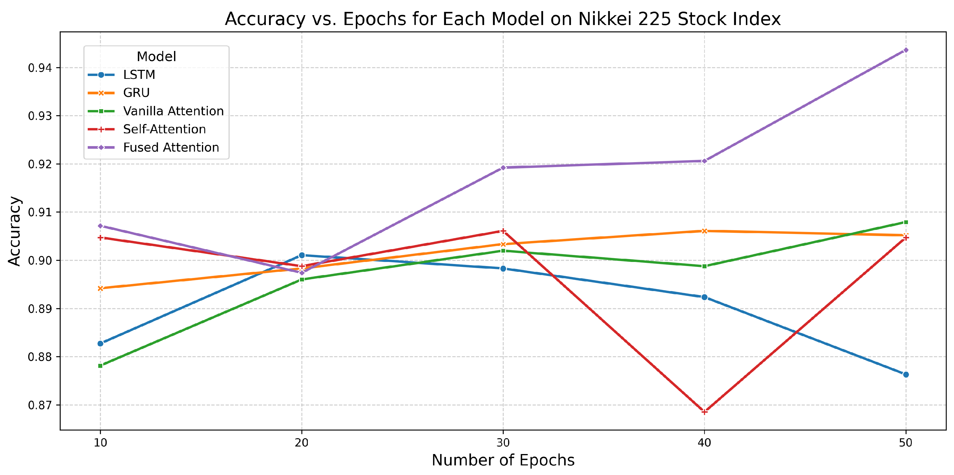
6.6. Performance of All Models on Nikkei 225 Stock Index
| Model | Epochs | Accuracy | AUC | Training Time (s) |
|---|---|---|---|---|
| LSTM | 10 | 0.8827 | 0.9651 | 8.7356 |
| 20 | 0.9011 | 0.9696 | 23.6938 | |
| 30 | 0.8983 | 0.9717 | 24.0915 | |
| 40 | 0.8924 | 0.9727 | 29.1918 | |
| 50 | 0.8763 | 0.9720 | 39.9231 | |
| GRU | 10 | 0.8942 | 0.9647 | 6.1163 |
| 20 | 0.8983 | 0.9695 | 11.1740 | |
| 30 | 0.9033 | 0.9715 | 19.4970 | |
| 40 | 0.9061 | 0.9727 | 21.4837 | |
| 50 | 0.9052 | 0.9725 | 27.6272 | |
| Vanilla Attention | 10 | 0.8781 | 0.9643 | 7.7629 |
| 20 | 0.8960 | 0.9695 | 15.4814 | |
| 30 | 0.9020 | 0.9718 | 22.8225 | |
| 40 | 0.8988 | 0.9725 | 33.2535 | |
| 50 | 0.9079 | 0.9726 | 41.2992 | |
| Self-Attention | 10 | 0.9047 | 0.9704 | 11.1087 |
| 20 | 0.8988 | 0.9721 | 22.3048 | |
| 30 | 0.9061 | 0.9727 | 32.5559 | |
| 40 | 0.8685 | 0.9723 | 42.5713 | |
| 50 | 0.9047 | 0.9726 | 54.2201 | |
| Fused Attention | 10 | 0.9072 | 0.9775 | 11.6053 |
| 20 | 0.8974 | 0.9711 | 23.6152 | |
| 30 | 0.9192 | 0.9824 | 34.8730 | |
| 40 | 0.9206 | 0.9834 | 45.7169 | |
| 50 | 0.9436 | 0.9876 | 57.6205 |

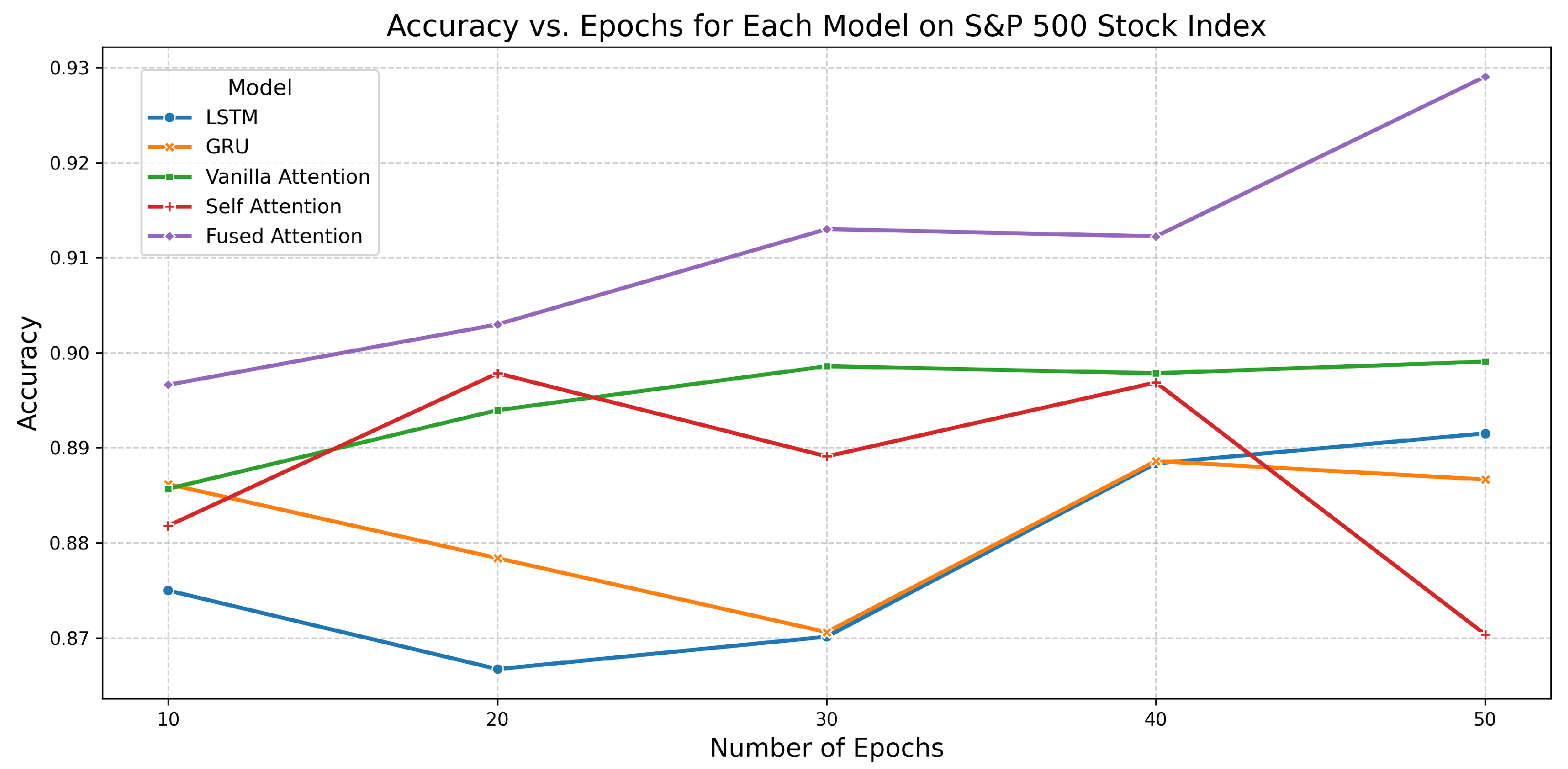
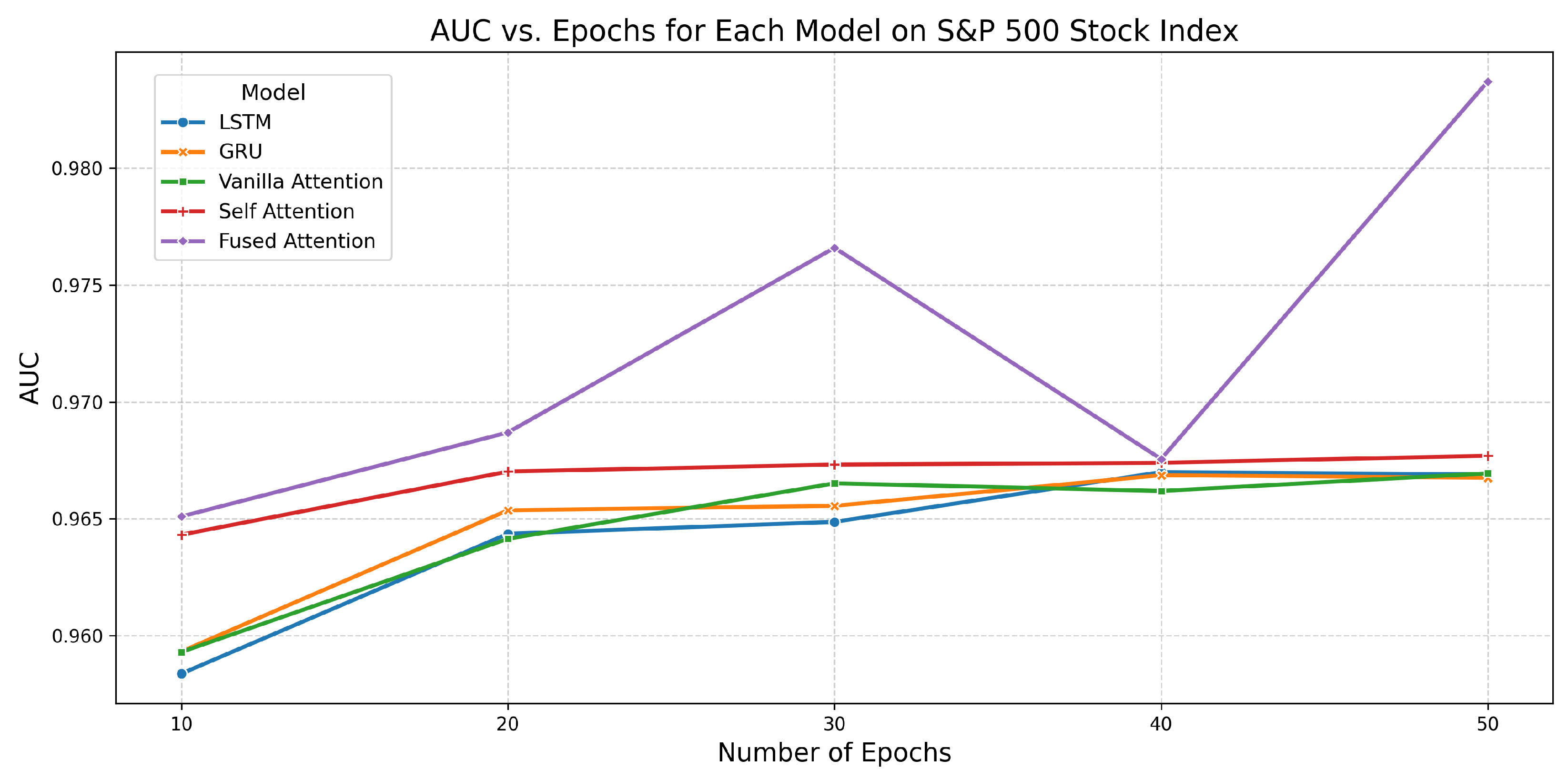
6.7. Performance of All Models on S&P 500 Stock Index
| Model | Epochs | Accuracy | AUC | Training Time (s) |
|---|---|---|---|---|
| LSTM | 10 | 0.8750 | 0.9584 | 14.2380 |
| 20 | 0.8667 | 0.9644 | 28.8773 | |
| 30 | 0.8701 | 0.9649 | 41.3208 | |
| 40 | 0.8883 | 0.9670 | 54.5288 | |
| 50 | 0.8915 | 0.9669 | 67.5416 | |
| GRU | 10 | 0.8862 | 0.9593 | 10.7352 |
| 20 | 0.8784 | 0.9654 | 19.7192 | |
| 30 | 0.8706 | 0.9656 | 31.7420 | |
| 40 | 0.8886 | 0.9669 | 41.1791 | |
| 50 | 0.8866 | 0.9667 | 51.7076 | |
| Vanilla Attention | 10 | 0.8857 | 0.9593 | 15.9441 |
| 20 | 0.8939 | 0.9641 | 29.2153 | |
| 30 | 0.8986 | 0.9665 | 43.6378 | |
| 40 | 0.8978 | 0.9662 | 57.3505 | |
| 50 | 0.8991 | 0.9669 | 72.2488 | |
| Self-Attention | 10 | 0.8818 | 0.9643 | 19.7511 |
| 20 | 0.8978 | 0.9670 | 39.3778 | |
| 30 | 0.8891 | 0.9673 | 60.6932 | |
| 40 | 0.8969 | 0.9674 | 78.0388 | |
| 50 | 0.8703 | 0.9677 | 99.8812 | |
| Fused Attention | 10 | 0.8966 | 0.9651 | 20.9063 |
| 20 | 0.9030 | 0.9687 | 41.7439 | |
| 30 | 0.9130 | 0.9766 | 65.2541 | |
| 40 | 0.9122 | 0.9676 | 82.2037 | |
| 50 | 0.9291 | 0.9837 | 103.3167 |
6.8. Performance of All Models on Shanghai Stock Index
| Model | Epochs | Accuracy | AUC | Training Time (s) |
|---|---|---|---|---|
| LSTM | 10 | 0.8156 | 0.9028 | 2.5063 |
| 20 | 0.8178 | 0.9152 | 4.9480 | |
| 30 | 0.8341 | 0.9214 | 6.6090 | |
| 40 | 0.8370 | 0.9261 | 9.1610 | |
| 50 | 0.8437 | 0.9333 | 11.5554 | |
| GRU | 10 | 0.8170 | 0.9034 | 1.7150 |
| 20 | 0.8200 | 0.9141 | 4.3073 | |
| 30 | 0.8296 | 0.9220 | 5.3555 | |
| 40 | 0.8356 | 0.9269 | 8.6228 | |
| 50 | 0.8378 | 0.9343 | 9.8929 | |
| Vanilla Attention | 10 | 0.7911 | 0.9029 | 2.4022 |
| 20 | 0.8215 | 0.9142 | 4.8537 | |
| 30 | 0.8252 | 0.9197 | 7.9445 | |
| 40 | 0.8207 | 0.9257 | 10.3482 | |
| 50 | 0.8407 | 0.9306 | 12.4405 | |
| Self-Attention | 10 | 0.7970 | 0.9179 | 3.3445 |
| 20 | 0.8207 | 0.9323 | 7.8554 | |
| 30 | 0.8556 | 0.9376 | 11.5627 | |
| 40 | 0.8615 | 0.9512 | 19.2510 | |
| 50 | 0.8719 | 0.9571 | 20.3122 | |
| Fused Attention | 10 | 0.8400 | 0.9283 | 4.2346 |
| 20 | 0.8333 | 0.9425 | 7.2577 | |
| 30 | 0.8615 | 0.9446 | 11.0987 | |
| 40 | 0.8696 | 0.9563 | 15.3568 | |
| 50 | 0.8730 | 0.9577 | 19.8575 |
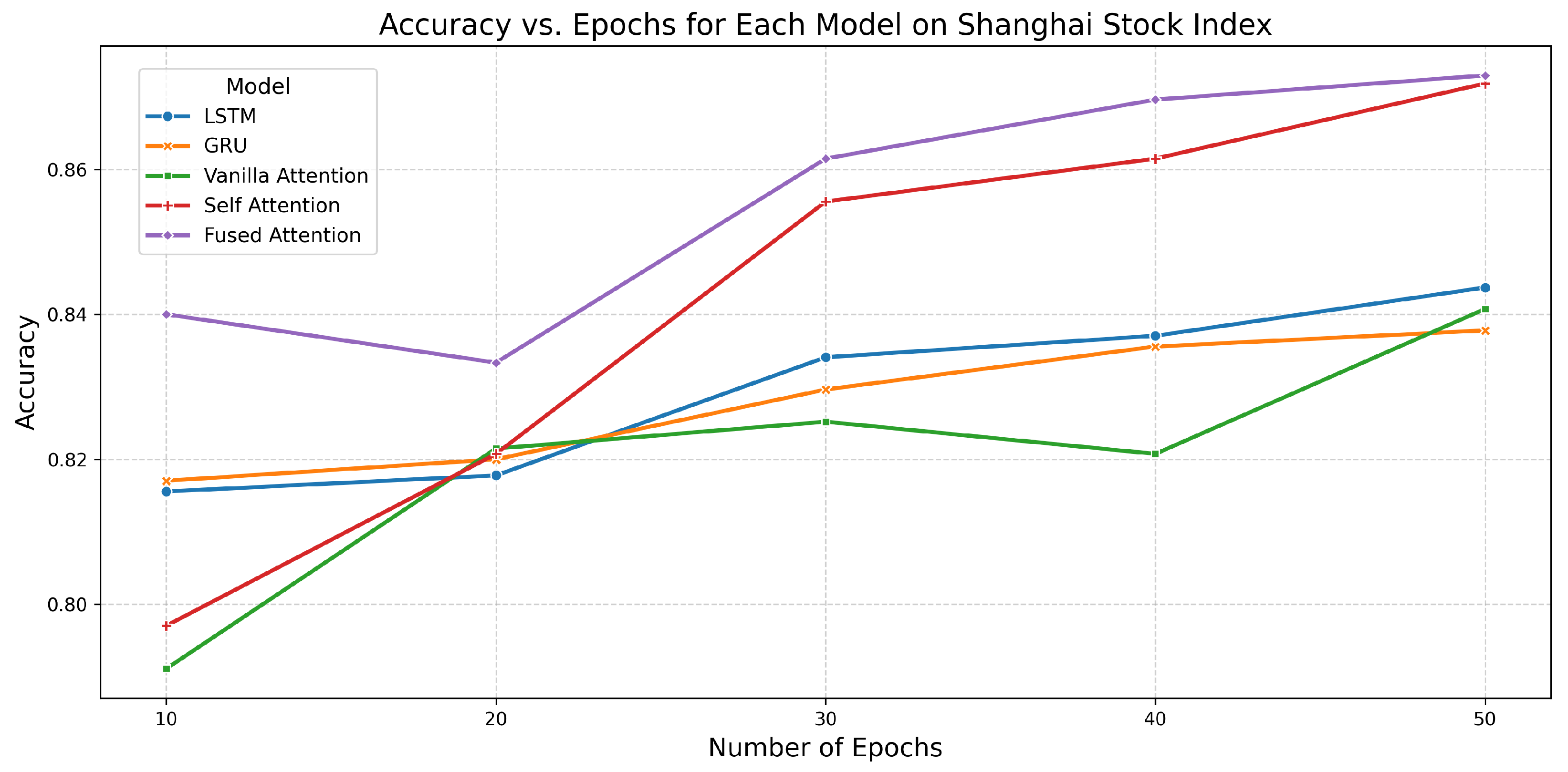
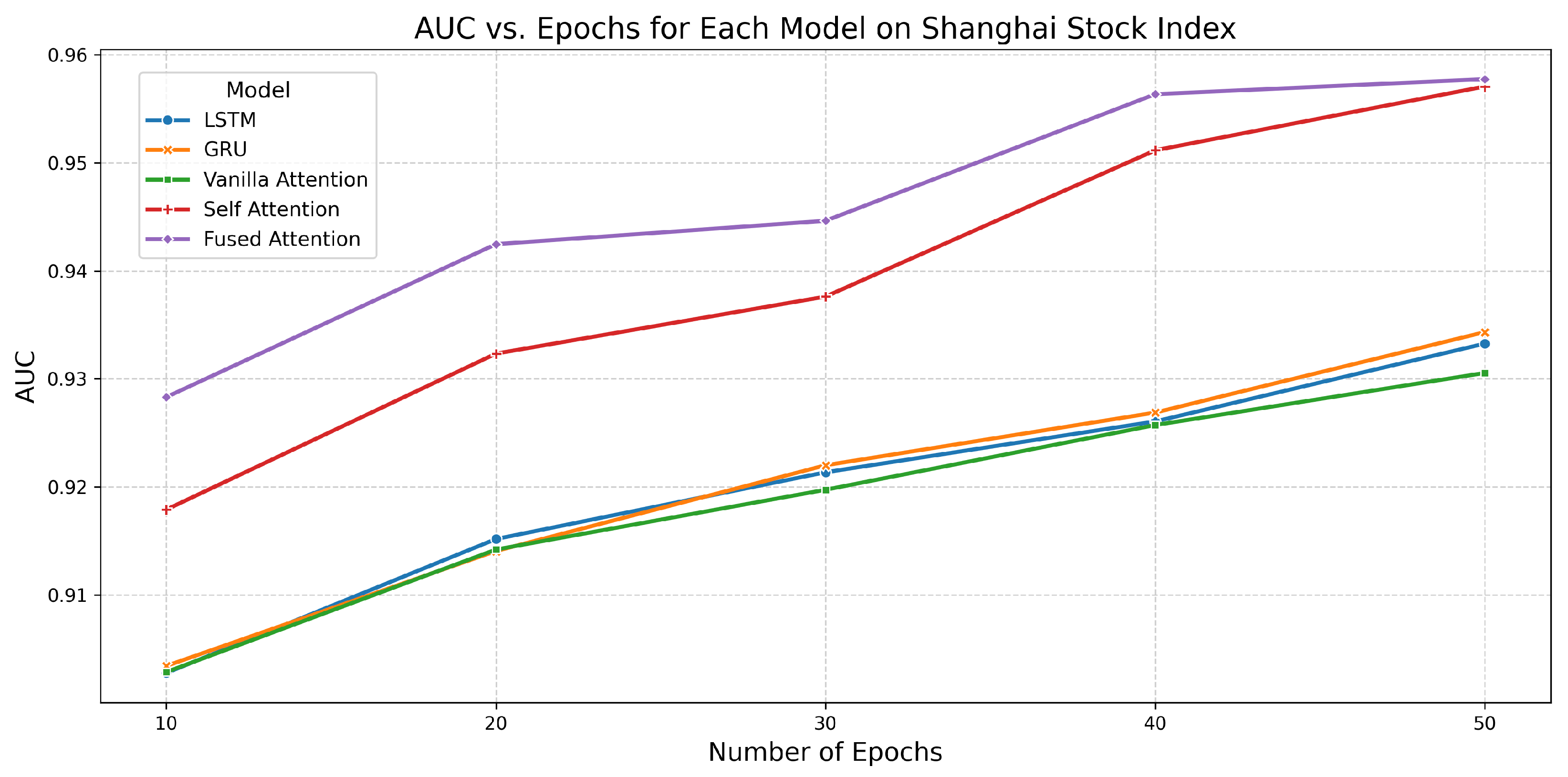
6.9. Performance of All Models on NIFTY 50 Stock Index
| Model | Epochs | Accuracy | AUC | Training Time (s) |
|---|---|---|---|---|
| LSTM | 10 | 0.8241 | 0.9169 | 2.0056 |
| 20 | 0.8517 | 0.9463 | 3.3540 | |
| 30 | 0.8638 | 0.9531 | 6.6336 | |
| 40 | 0.8759 | 0.9572 | 6.3785 | |
| 50 | 0.8862 | 0.9589 | 8.3614 | |
| GRU | 10 | 0.8328 | 0.9269 | 1.0515 |
| 20 | 0.8655 | 0.9487 | 2.1409 | |
| 30 | 0.8655 | 0.9534 | 3.2570 | |
| 40 | 0.8724 | 0.9568 | 5.7098 | |
| 50 | 0.8845 | 0.9595 | 5.6378 | |
| Vanilla Attention | 10 | 0.8293 | 0.9243 | 1.5489 |
| 20 | 0.8483 | 0.9471 | 4.1955 | |
| 30 | 0.8707 | 0.9537 | 5.7672 | |
| 40 | 0.8707 | 0.9575 | 7.4089 | |
| 50 | 0.8741 | 0.9591 | 7.7112 | |
| Self-Attention | 10 | 0.8569 | 0.9511 | 2.3682 |
| 20 | 0.8828 | 0.9610 | 5.2289 | |
| 30 | 0.8603 | 0.9623 | 5.8652 | |
| 40 | 0.8879 | 0.9654 | 9.9230 | |
| 50 | 0.8948 | 0.9672 | 16.2260 | |
| Fused Attention | 10 | 0.8552 | 0.9610 | 2.1109 |
| 20 | 0.8897 | 0.9631 | 5.3348 | |
| 30 | 0.8734 | 0.9677 | 6.4097 | |
| 40 | 0.8979 | 0.9685 | 9.9200 | |
| 50 | 0.8983 | 0.9678 | 11.8721 |
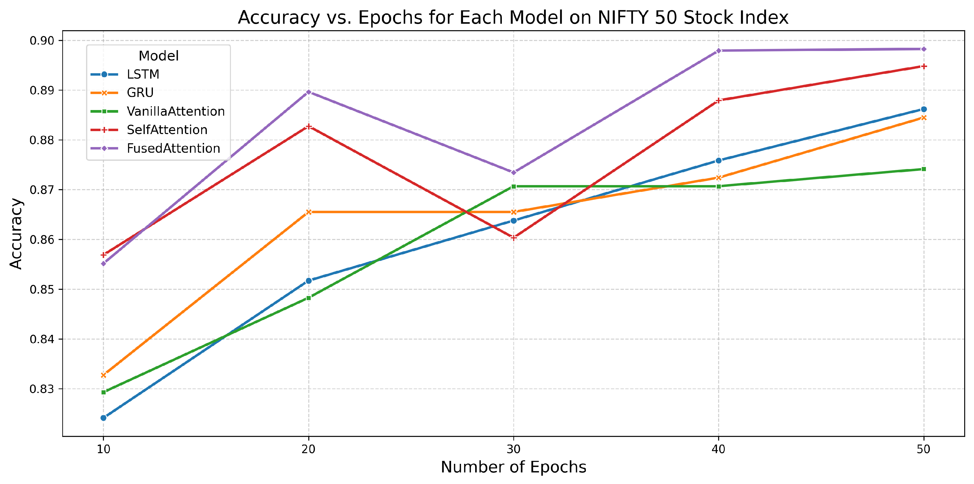

7. Comparative Analysis of Model Performance
7.1. Accuracy Analysis
7.2. AUC Analysis
7.3. Critical Observations
8. Ablation Study
8.1. Individual Attention Ablation Study: Sparse, Global, and Random Attention
8.2. Remove-One Ablation Study
8.2.1. Analysis of Remove-One Ablation on DJUS, NYSE AMEX, BSE, DAX, and NASDAQ Stock Indices
8.2.2. Analysis of Remove-One Ablation on Nikkei 225, S&P 500, Shanghai, and NIFTY 50 Stock Indices
9. Conclusions and Future Work
Author Contributions
Funding
Institutional Review Board Statement
Informed Consent Statement
Data Availability Statement
Conflicts of Interest
References
- González-Rivera, G.; Lee, T.H. Financial Forecasting, Nonlinear Time Series. In Encyclopedia of Complexity and Systems Science; Meyers, R.A., Ed.; Springer: New York, NY, USA, 2009; pp. 3475–3504. [Google Scholar] [CrossRef]
- Pai, P.F.; Lin, C.S. A Hybrid ARIMA and Support Vector Machines Model in Stock Price Forecasting. Omega 2005, 33, 497–505. [Google Scholar] [CrossRef]
- Wei, W.W.S. Forecasting with ARIMA Processes. In International Encyclopedia of Statistical Science; Lovric, M., Ed.; Springer: Berlin/Heidelberg, Germany, 2011; pp. 534–536. [Google Scholar] [CrossRef]
- Long, W.; Lu, Z.; Cui, L. Deep Learning-Based Feature Engineering for Stock Price Movement Prediction. Knowl.-Based Syst. 2019, 164, 163–173. [Google Scholar] [CrossRef]
- Liu, G.; Wang, X. A Numerical-Based Attention Method for Stock Market Prediction with Dual Information. IEEE Access 2019, 7, 7357–7367. [Google Scholar] [CrossRef]
- Chen, J.; Xie, L.; Lin, W.; Wu, Y.; Xu, H. Multi-Granularity Spatio-Temporal Correlation Networks for Stock Trend Prediction. IEEE Access 2024, 12, 67219–67232. [Google Scholar] [CrossRef]
- Luo, A.; Zhong, L.; Wang, J.; Wang, Y.; Li, S.; Tai, W. Short-Term Stock Correlation Forecasting Based on CNN-BiLSTM Enhanced by Attention Mechanism. IEEE Access 2024, 12, 29617–29632. [Google Scholar] [CrossRef]
- Lam, M. Neural network techniques for financial performance prediction: Integrating fundamental and technical analysis. Decis. Support Syst. 2004, 37, 567–581. [Google Scholar] [CrossRef]
- Kara, Y.; Boyacioglu, M.A.; Kaan Baykan, Ö. Predicting Direction of Stock Price Index Movement Using Artificial Neural Networks and Support Vector Machines: The Sample of the Istanbul Stock Exchange. Expert Syst. Appl. 2011, 38, 5311–5319. [Google Scholar] [CrossRef]
- Patel, J.; Shah, S.; Thakkar, P.; Kotecha, K. Predicting Stock and Stock Price Index Movement Using Trend Deterministic Data Preparation and Machine Learning Techniques. Expert Syst. Appl. 2015, 42, 259–268. [Google Scholar] [CrossRef]
- Ballings, M.; Poel, D.V.D.; Hespeels, N.; Gryp, R. Evaluating Multiple Classifiers for Stock Price Direction Prediction. Expert Syst. Appl. 2015, 42, 7046–7056. [Google Scholar] [CrossRef]
- Zhang, X.D.; Li, A.; Pan, R. Stock Trend Prediction Based on a New Status Box Method and AdaBoost Probabilistic Support Vector Machine. Appl. Soft Comput. 2016, 49, 385–398. [Google Scholar] [CrossRef]
- Fischer, T.; Krauss, C. Deep Learning with Long Short-Term Memory Networks for Financial Market Predictions. Eur. J. Oper. Res. 2018, 270, 654–669. [Google Scholar] [CrossRef]
- Lai, G.; Chang, W.C.; Yang, Y.; Liu, H. Modeling long- and short-term temporal patterns with deep neural networks. In Proceedings of the 41st International ACM SIGIR Conference on Research and Development in Information Retrieval, SIGIR 2018, Ann Arbor, MI, USA, 8–12 July 2018; pp. 95–104. [Google Scholar] [CrossRef]
- Dosovitskiy, A.; Beyer, L.; Kolesnikov, A.; Weissenborn, D.; Zhai, X.; Unterthiner, T.; Dehghani, M.; Minderer, M.; Heigold, G.; Gelly, S.; et al. An Image is Worth 16 × 16 Words: Transformers for Image Recognition at Scale. In Proceedings of the ICLR 2021—9th International Conference on Learning Representations, Virtual, 3–7 May 2021. [Google Scholar]
- Zeng, A.; Chen, M.; Zhang, L.; Xu, Q. Are Transformers Effective for Time Series Forecasting? In Proceedings of the AAAI Conference on Artificial Intelligence, Washington, DC, USA, 7–14 February 2023; Volume 37, pp. 11121–11128. [Google Scholar] [CrossRef]
- Qiu, J.; Wang, B.; Zhou, C. Forecasting stock prices with long-short term memory neural network based on attention mechanism. PLoS ONE 2020, 15, e0227222. [Google Scholar] [CrossRef]
- Zhou, H.; Zhang, S.; Peng, J.; Zhang, S.; Li, J.; Xiong, H.; Zhang, W. Informer: Beyond Efficient Transformer for Long Sequence Time-Series Forecasting. In Proceedings of the AAAI Conference on Artificial Intelligence, Virtual, 2–9 February 2021; Volume 35, pp. 11106–11115. [Google Scholar] [CrossRef]
- Zhou, T.; Ma, Z.; Wen, Q.; Wang, X.; Sun, L.; Jin, R. FEDformer: Frequency Enhanced Decomposed Transformer for Long-Term Series Forecasting. In Proceedings of the 39th International Conference on Machine Learning (ICML 2022), Baltimore, MD, USA, 17–23 July 2022; Proceedings of Machine Learning Research. Chaudhuri, K., Jegelka, S., Song, L., Szepesvari, C., Niu, G., Sabato, S., Eds.; Volume 162, pp. 27268–27286. Available online: https://proceedings.mlr.press/v162/zhou22g.html (accessed on 21 August 2025).
- Zhang, Y.; Yan, J. Crossformer: Transformer Utilizing Cross-Dimension Dependency for Multivariate Time Series Forecasting. In Proceedings of the International Conference on Learning Representations, Kigali, Rwanda, 1–5 May 2023. [Google Scholar]
- Nie, Y.; Nguyen, N.H.; Sinthong, P.; Kalagnanam, J. A Time Series is Worth 64 Words: Long-term Forecasting with Transformers. In Proceedings of the 11th International Conference on Learning Representations, ICLR 2023, Kigali, Rwanda, 1–5 May 2023. [Google Scholar]
- Cheng, R.; Li, Q. Modeling the Momentum Spillover Effect for Stock Prediction via Attribute-Driven Graph Attention Networks. In Proceedings of the AAAI Conference on Artificial Intelligence, Virtual, 2–9 February 2021. [Google Scholar]
- Lu, W.; Li, J.; Wang, J.; Qin, L. A CNN-BiLSTM-AM Method for Stock Price Prediction. Neural Comput. Appl. 2021, 33, 4741–4753. [Google Scholar] [CrossRef]
- Su, H.; Wang, X.; Qin, Y.; Chen, Q. Attention-based adaptive spatial–temporal hypergraph convolutional networks for stock price trend prediction. Expert Syst. Appl. 2024, 238, 121899. [Google Scholar] [CrossRef]
- Zhang, Y.; Wu, R.; Dascalu, S.M.; Harris, F.C. Sparse transformer with local and seasonal adaptation for multivariate time series forecasting. Sci. Rep. 2024, 14, 15909. [Google Scholar] [CrossRef]
- Dong, Y.; Hao, Y. A Stock Prediction Method Based on Multidimensional and Multilevel Feature Dynamic Fusion. Electronics 2024, 13, 4111. [Google Scholar] [CrossRef]
- Bustos, O.; Pomares-Quimbaya, A. Stock Market Movement Forecast: A Systematic Review. Expert Syst. Appl. 2020, 156, 113464. [Google Scholar] [CrossRef]
- Nabipour, M.; Nayyeri, P.; Jabani, H.; Shahab, S.; Mosavi, A. Predicting Stock Market Trends Using Machine Learning and Deep Learning Algorithms via Continuous and Binary Data: A Comparative Analysis. IEEE Access 2020, 8, 150199–150212. [Google Scholar] [CrossRef]
- Lee, H.; Kim, J.H.; Jung, H.S. Deep-learning-based stock market prediction incorporating ESG sentiment and technical indicators. Sci. Rep. 2024, 14, 10262. [Google Scholar] [CrossRef] [PubMed]
- Chong, E.; Han, C.; Park, F.C. Deep Learning Networks for Stock Market Analysis and Prediction: Methodology, Data Representations, and Case Studies. Expert Syst. Appl. 2017, 83, 187–205. [Google Scholar] [CrossRef]
- Jiang, W. Applications of Deep Learning in Stock Market Prediction: Recent Progress. Expert Syst. Appl. 2021, 184, 115537. [Google Scholar] [CrossRef]
- Sun, Z.; Harit, A.; Cristea, A.I.; Wang, J.; Lio, P. MONEY: Ensemble learning for stock price movement prediction via a convolutional network with adversarial hypergraph model. AI Open 2023, 4, 165–174. [Google Scholar] [CrossRef]
- Vaswani, A.; Shazeer, N.; Parmar, N.; Uszkoreit, J.; Jones, L.; Gomez, A.N.; Kaiser, Ł.; Polosukhin, I. Attention Is All You Need. Adv. Neural Inf. Process. Syst. 2017, 30, 5998–6008. [Google Scholar]
- Mao, W.; Liu, P.; Huang, J. SF-Transformer: A Mutual Information-Enhanced Transformer Model with Spot-Forward Parity for Forecasting Long-Term Chinese Stock Index Futures Prices. Entropy 2024, 26, 478. [Google Scholar] [CrossRef]
- Yang, S.; Ding, Y.; Xie, B.; Guo, Y.; Bai, X.; Qian, J.; Gao, Y.; Wang, W.; Ren, J. Advancing Financial Forecasts: A Deep Dive into Memory Attention and Long-Distance Loss in Stock Price Predictions. Appl. Sci. 2023, 13, 12160. [Google Scholar] [CrossRef]
- Peng, H.; Pappas, N.; Yogatama, D.; Schwartz, R.; Smith, N.A.; Kong, L. Random Feature Attention. arXiv 2021, arXiv:2103.02143. [Google Scholar] [CrossRef]
- Zheng, L.; Wang, C.; Kong, L. Linear Complexity Randomized Self-Attention Mechanism. arXiv 2022, arXiv:2204.04667. [Google Scholar] [CrossRef]
| Reference | Technique | Attention | Task |
|---|---|---|---|
| [8] | Backpropagation Neural Network | No | Time-Series Classification |
| [9] | Neural Network and Support Vector Machine | No | Time-Series Classification |
| [10] | Neural Network, Support Vector Machine, Random Forest, and Naïve Bayes | No | Time-Series Classification |
| [11] | Kernel Factory | No | Time-Series Classification |
| [12] | Genetic Algorithm and Support Vector Machine | No | Time-Series Classification |
| [13] | LSTM | No | Time-Series Classification |
| [14] | CNN and RNN | No | Time-Series Forecasting |
| [15] | Transformer | Yes | Image Classification |
| [16] | Transformer | Yes | Time-Series Forecasting |
| [17] | LSTM with Attention | Yes | Time-Series Forecasting |
| [18] | Informer | Yes | Time-Series Forecasting |
| [19] | FEDformer | Yes | Time-Series Forecasting |
| [20] | Crossformer | Yes | Time-Series Forecasting |
| [21] | PatchTST | Yes | Time-Series Forecasting |
| [22] | Graph Attention Network | Yes | Time-Series Forecasting |
| [23] | BiLSTM, Transformer | Yes | Time-Series Forecasting |
| [24] | Noise-Aware Attention | Yes | Time-Series Forecasting |
| [25] | DozerFormer | Yes | Time-Series Forecasting |
| [26] | Dynamic Feature Fusion Frameworks | Yes | Time-Series Forecasting |
| Our Model: SGR-Net | Fusion of Sparse, Global, and Random Attention | Yes | Time-Series Classification |
| Stock Index | Time Span | Training Data (70%) | Testing Data (30%) | ||||
|---|---|---|---|---|---|---|---|
| Up-Trends | Down-Trends | Total Instances | Up-Trends | Down-Trends | Total Instances | ||
| DJUS Index | April 2005–July 2016 | 997 | 827 | 1824 | 438 | 344 | 782 |
| NYSE AMEX Index | January 1996–July 2016 | 1957 | 1668 | 3625 | 850 | 704 | 1554 |
| BSE Index | January 2005–December 2015 | 1020 | 892 | 1912 | 437 | 382 | 819 |
| DAX Index | January 1991–July 2016 | 2413 | 2114 | 4527 | 1044 | 897 | 1941 |
| NASDAQ Index | January 2005–December 2015 | 1058 | 865 | 1923 | 446 | 378 | 824 |
| Nikkei 225 Index | January 1987–July 2016 | 2609 | 2483 | 5092 | 1115 | 1067 | 2182 |
| S&P 500 Index | January 1962–July 2016 | 5118 | 4473 | 9591 | 2146 | 1964 | 4110 |
| Shanghai Stock Exchange Index | January 1998–July 2016 | 1679 | 1470 | 3149 | 685 | 665 | 1350 |
| NIFTY 50 Index | January 2008–December 2015 | 709 | 644 | 1353 | 300 | 279 | 579 |
| Hyperparameter | Value/Description |
|---|---|
| LSTM hidden units | 128 |
| Batch size | 32 |
| Learning rate | 0.001 (Adam optimizer) |
| Loss function | CrossEntropyLoss |
| Optimizer | Adam |
| Epochs | 10, 20, 30, 40, and 50 (all models); 10–100 in steps of 10 (SGR-Net) |
| Model | Epochs | Accuracy | AUC | Training Time (s) |
|---|---|---|---|---|
| Fused Attention | 10 | 0.8299 | 0.9144 | 2.5265 |
| 20 | 0.8333 | 0.9265 | 4.1947 | |
| 30 | 0.8461 | 0.9345 | 6.7247 | |
| 40 | 0.8581 | 0.9401 | 8.1700 | |
| 50 | 0.8581 | 0.9442 | 10.9043 | |
| 60 | 0.8632 | 0.9467 | 12.0609 | |
| 70 | 0.8542 | 0.9493 | 15.4306 | |
| 80 | 0.8721 | 0.9481 | 18.3172 | |
| 90 | 0.8555 | 0.9469 | 20.6902 | |
| 100 | 0.8299 | 0.9535 | 23.8549 |
| Model | Epochs | Accuracy | AUC | Training Time (s) |
|---|---|---|---|---|
| Fused Attention | 10 | 0.8900 | 0.9665 | 5.2198 |
| 20 | 0.8993 | 0.9697 | 8.7127 | |
| 30 | 0.9145 | 0.9718 | 13.9070 | |
| 40 | 0.9222 | 0.9728 | 17.9407 | |
| 50 | 0.9428 | 0.9824 | 22.6548 | |
| 60 | 0.9445 | 0.9717 | 30.4493 | |
| 70 | 0.9103 | 0.9690 | 43.5673 | |
| 80 | 0.9048 | 0.9719 | 54.3972 | |
| 90 | 0.9015 | 0.9713 | 72.3547 | |
| 100 | 0.8758 | 0.9674 | 87.3527 |
| Model | Epochs | Accuracy | AUC | Training Time (s) |
|---|---|---|---|---|
| Fused Attention | 10 | 0.9098 | 0.9685 | 5.3015 |
| 20 | 0.9161 | 0.9691 | 9.1033 | |
| 30 | 0.9085 | 0.9690 | 14.7980 | |
| 40 | 0.9254 | 0.9710 | 19.3200 | |
| 50 | 0.9324 | 0.9793 | 21.9127 | |
| 60 | 0.9285 | 0.9697 | 25.6869 | |
| 70 | 0.9112 | 0.9704 | 29.3633 | |
| 80 | 0.9024 | 0.9698 | 33.9195 | |
| 90 | 0.8976 | 0.9707 | 36.6264 | |
| 100 | 0.9098 | 0.9716 | 42.2621 |
| Model | Epochs | Accuracy | AUC | Training Time (s) |
|---|---|---|---|---|
| Fused Attention | 10 | 0.8891 | 0.9715 | 10.0830 |
| 20 | 0.8936 | 0.9749 | 17.8837 | |
| 30 | 0.9126 | 0.9784 | 27.9773 | |
| 40 | 0.8980 | 0.9748 | 36.8110 | |
| 50 | 0.9208 | 0.9840 | 44.7582 | |
| 60 | 0.9101 | 0.9748 | 55.8708 | |
| 70 | 0.9031 | 0.9756 | 65.7375 | |
| 80 | 0.8903 | 0.9756 | 73.8886 | |
| 90 | 0.9098 | 0.9771 | 83.1955 | |
| 100 | 0.8918 | 0.9763 | 91.1857 |
| Model | Epochs | Accuracy | AUC | Training Time (s) |
|---|---|---|---|---|
| Fused Attention | 10 | 0.9127 | 0.9776 | 5.5162 |
| 20 | 0.9145 | 0.9792 | 7.9996 | |
| 30 | 0.9219 | 0.9811 | 13.3201 | |
| 40 | 0.9297 | 0.9799 | 18.2401 | |
| 50 | 0.9364 | 0.9888 | 22.0903 | |
| 60 | 0.9355 | 0.9882 | 25.8913 | |
| 70 | 0.9188 | 0.9787 | 28.6653 | |
| 80 | 0.8715 | 0.9797 | 32.0084 | |
| 90 | 0.9164 | 0.9793 | 35.9114 | |
| 100 | 0.9176 | 0.9783 | 40.5604 |
| Model | Epochs | Accuracy | AUC | Training Time (s) |
|---|---|---|---|---|
| Fused Attention | 10 | 0.9072 | 0.9775 | 11.8397 |
| 20 | 0.8974 | 0.9711 | 19.1397 | |
| 30 | 0.9192 | 0.9824 | 25.6087 | |
| 40 | 0.9206 | 0.9834 | 34.4480 | |
| 50 | 0.9436 | 0.9876 | 41.7566 | |
| 60 | 0.9456 | 0.9829 | 49.7582 | |
| 70 | 0.8931 | 0.9718 | 57.6543 | |
| 80 | 0.8992 | 0.9753 | 66.6440 | |
| 90 | 0.9104 | 0.9837 | 75.8100 | |
| 100 | 0.9075 | 0.9748 | 85.2727 |
| Model | Epochs | Accuracy | AUC | Training Time (s) |
|---|---|---|---|---|
| Fused Attention | 10 | 0.8966 | 0.9651 | 20.9063 |
| 20 | 0.9030 | 0.9687 | 41.7439 | |
| 30 | 0.9130 | 0.9766 | 65.2541 | |
| 40 | 0.9122 | 0.9676 | 82.2037 | |
| 50 | 0.9291 | 0.9837 | 103.3167 | |
| 60 | 0.8922 | 0.9692 | 123.0970 | |
| 70 | 0.9022 | 0.9712 | 144.4847 | |
| 80 | 0.8959 | 0.9694 | 163.6611 | |
| 90 | 0.9015 | 0.9719 | 189.9799 | |
| 100 | 0.9032 | 0.9730 | 214.2635 |
| Model | Epochs | Accuracy | AUC | Training Time (s) |
|---|---|---|---|---|
| Fused Attention | 10 | 0.8400 | 0.9283 | 4.2346 |
| 20 | 0.8333 | 0.9425 | 7.2577 | |
| 30 | 0.8615 | 0.9446 | 11.0987 | |
| 40 | 0.8696 | 0.9563 | 15.3568 | |
| 50 | 0.8730 | 0.9577 | 19.8575 | |
| 60 | 0.8733 | 0.9593 | 27.4802 | |
| 70 | 0.8748 | 0.9597 | 34.3601 | |
| 80 | 0.8748 | 0.9604 | 40.7298 | |
| 90 | 0.8459 | 0.9583 | 46.8047 | |
| 100 | 0.8281 | 0.9557 | 54.0861 |
| Model | Epochs | Accuracy | AUC | Training Time (s) |
|---|---|---|---|---|
| Fused Attention | 10 | 0.8552 | 0.9610 | 2.1109 |
| 20 | 0.8897 | 0.9631 | 5.3348 | |
| 30 | 0.8734 | 0.9677 | 6.4097 | |
| 40 | 0.8979 | 0.9685 | 9.9200 | |
| 50 | 0.8983 | 0.9678 | 11.8721 | |
| 60 | 0.8690 | 0.9656 | 15.5928 | |
| 70 | 0.8828 | 0.9683 | 18.2711 | |
| 80 | 0.8914 | 0.9683 | 21.8305 | |
| 90 | 0.8724 | 0.9682 | 23.9187 | |
| 100 | 0.8948 | 0.9689 | 27.5492 |
| Model | DJUS | NYSE AMEX | BSE | DAX | NASDAQ | Nikkei 225 | S&P 500 | Shanghai Stock Exchange | NIFTY 50 |
|---|---|---|---|---|---|---|---|---|---|
| LSTM | 0.8338 | 0.9060 | 0.9122 | 0.9016 | 0.9236 | 0.9011 | 0.8915 | 0.8437 | 0.8862 |
| GRU | 0.8286 | 0.9015 | 0.9061 | 0.9011 | 0.9236 | 0.9061 | 0.8886 | 0.8378 | 0.8845 |
| Vanilla Attention | 0.8312 | 0.9009 | 0.9085 | 0.8985 | 0.9236 | 0.9079 | 0.8991 | 0.8407 | 0.8741 |
| Self-Attention | 0.8529 | 0.8970 | 0.9110 | 0.9109 | 0.9273 | 0.9061 | 0.8978 | 0.8719 | 0.8948 |
| Fused Attention (SGR-Net) | 0.8581 | 0.9428 | 0.9324 | 0.9208 | 0.9364 | 0.9436 | 0.9291 | 0.8730 | 0.8983 |
| Model | DJUS | NYSE AMEX | BSE | DAX | NASDAQ | Nikkei 225 | S&P 500 | Shanghai Stock Exchange | NIFTY 50 |
|---|---|---|---|---|---|---|---|---|---|
| LSTM | 0.9164 | 0.9703 | 0.9694 | 0.9739 | 0.9790 | 0.9727 | 0.9669 | 0.9333 | 0.9589 |
| GRU | 0.9170 | 0.9696 | 0.9697 | 0.9743 | 0.9794 | 0.9727 | 0.9669 | 0.9343 | 0.9595 |
| Vanilla Attention | 0.9162 | 0.9702 | 0.9696 | 0.9726 | 0.9793 | 0.9726 | 0.9669 | 0.9306 | 0.9591 |
| Self-Attention | 0.9393 | 0.9726 | 0.9698 | 0.9757 | 0.9796 | 0.9727 | 0.9677 | 0.9571 | 0.9672 |
| Fused Attention (SGR-Net) | 0.9442 | 0.9824 | 0.9793 | 0.9840 | 0.9888 | 0.9876 | 0.9837 | 0.9577 | 0.9685 |
| Model Variant | Metric | DJUS | NYSE AMEX | BSE | DAX | NASDAQ |
|---|---|---|---|---|---|---|
| Only Sparse | Accuracy | 0.8352 [0.8150–0.8550] | 0.9072 [0.8920–0.9190] | 0.9127 [0.8940–0.9290] | 0.9048 [0.8890–0.9180] | 0.9244 [0.9060–0.9400] |
| Precision | 0.8285 [0.8000–0.8540] | 0.8830 [0.8620–0.9020] | 0.8880 [0.8640–0.9100] | 0.8780 [0.8550–0.8980] | 0.8920 [0.8680–0.9140] | |
| Recall | 0.8421 [0.8150–0.8680] | 0.8895 [0.8690–0.9090] | 0.8975 [0.8750–0.9190] | 0.8910 [0.8700–0.9110] | 0.9035 [0.8800–0.9250] | |
| F1-score | 0.8351 [0.8100–0.8600] | 0.8862 [0.8680–0.9040] | 0.8927 [0.8730–0.9110] | 0.8842 [0.8660–0.9020] | 0.8973 [0.8770–0.9150] | |
| AUC | 0.9250 [0.9185–0.9310] | 0.9698 [0.9660–0.9735] | 0.9696 [0.9635–0.9755] | 0.9742 [0.9695–0.9790] | 0.9795 [0.9735–0.9850] | |
| Only Global | Accuracy | 0.8361 [0.8170–0.8560] | 0.9084 [0.8950–0.9200] | 0.9129 [0.8950–0.9290] | 0.9029 [0.8880–0.9160] | 0.9256 [0.9080–0.9410] |
| Precision | 0.8328 [0.8050–0.8570] | 0.8845 [0.8640–0.9040] | 0.8895 [0.8660–0.9120] | 0.8765 [0.8530–0.8990] | 0.8940 [0.8700–0.9160] | |
| Recall | 0.8442 [0.8180–0.8700] | 0.8880 [0.8680–0.9080] | 0.8988 [0.8770–0.9200] | 0.8887 [0.8680–0.9090] | 0.9052 [0.8820–0.9260] | |
| F1-score | 0.8383 [0.8140–0.8620] | 0.8862 [0.8680–0.9035] | 0.8940 [0.8750–0.9120] | 0.8825 [0.8650–0.9010] | 0.8989 [0.8790–0.9165] | |
| AUC | 0.9290 [0.9200–0.9380] | 0.9699 [0.9665–0.9738] | 0.9697 [0.9640–0.9752] | 0.9744 [0.9698–0.9790] | 0.9796 [0.9740–0.9852] | |
| Only Random | Accuracy | 0.8349 [0.8150–0.8550] | 0.9067 [0.8920–0.9180] | 0.9126 [0.8940–0.9290] | 0.9053 [0.8890–0.9180] | 0.9249 [0.9070–0.9400] |
| Precision | 0.8292 [0.8020–0.8540] | 0.8820 [0.8610–0.9010] | 0.8870 [0.8630–0.9100] | 0.8795 [0.8550–0.9000] | 0.8928 [0.8690–0.9150] | |
| Recall | 0.8410 [0.8140–0.8670] | 0.8865 [0.8660–0.9060] | 0.8979 [0.8750–0.9190] | 0.8905 [0.8700–0.9100] | 0.9041 [0.8810–0.9250] | |
| F1-score | 0.8344 [0.8100–0.8590] | 0.8842 [0.8660–0.9020] | 0.8923 [0.8730–0.9100] | 0.8848 [0.8670–0.9020] | 0.8981 [0.8780–0.9160] | |
| AUC | 0.9215 [0.9185–0.9300] | 0.9696 [0.9660–0.9732] | 0.9695 [0.9635–0.9750] | 0.9741 [0.9692–0.9788] | 0.9793 [0.9732–0.9848] | |
| SGR-Net | Accuracy | 0.8581 [0.8370–0.8780] | 0.9428 [0.9300–0.9560] | 0.9324 [0.9130–0.9490] | 0.9208 [0.9070–0.9350] | 0.9364 [0.9200–0.9520] |
| Precision | 0.9000 [0.8730–0.9250] | 0.9300 [0.9120–0.9460] | 0.9280 [0.9050–0.9490] | 0.9140 [0.8950–0.9310] | 0.9360 [0.9120–0.9560] | |
| Recall | 0.8800 [0.8520–0.9050] | 0.9360 [0.9180–0.9520] | 0.9260 [0.9030–0.9470] | 0.9180 [0.8980–0.9380] | 0.9380 [0.9140–0.9590] | |
| F1-score | 0.8900 [0.8640–0.9140] | 0.9330 [0.9160–0.9490] | 0.9270 [0.9070–0.9460] | 0.9160 [0.8980–0.9340] | 0.9370 [0.9150–0.9560] | |
| AUC | 0.9442 [0.9320–0.9570] | 0.9824 [0.9760–0.9880] | 0.9793 [0.9690–0.9880] | 0.9840 [0.9780–0.9890] | 0.9888 [0.9820–0.9940] |
| Model Variant | Metric | Nikkei 225 | S&P 500 | Shanghai | NIFTY 50 |
|---|---|---|---|---|---|
| Only Sparse | Accuracy | 0.9028 [0.8890–0.9150] | 0.8962 [0.8830–0.9070] | 0.8542 [0.8330–0.8730] | 0.8892 [0.8700–0.9070] |
| Precision | 0.8960 [0.8800–0.9110] | 0.8880 [0.8740–0.9010] | 0.8380 [0.8100–0.8640] | 0.8780 [0.8560–0.8980] | |
| Recall | 0.9070 [0.8920–0.9210] | 0.9010 [0.8880–0.9140] | 0.8720 [0.8480–0.8940] | 0.9000 [0.8790–0.9200] | |
| F1-score | 0.9015 [0.8860–0.9160] | 0.8945 [0.8820–0.9060] | 0.8540 [0.8330–0.8730] | 0.8890 [0.8700–0.9070] | |
| AUC | 0.9665 [0.9590–0.9730] | 0.9639 [0.9570–0.9710] | 0.9410 [0.9320–0.9500] | 0.9617 [0.9540–0.9690] | |
| Only Global | Accuracy | 0.9056 [0.8930–0.9180] | 0.8940 [0.8810–0.9060] | 0.8605 [0.8400–0.8790] | 0.8918 [0.8730–0.9100] |
| Precision | 0.9000 [0.8840–0.9160] | 0.8850 [0.8710–0.8980] | 0.8460 [0.8200–0.8700] | 0.8800 [0.8580–0.9000] | |
| Recall | 0.9100 [0.8940–0.9240] | 0.8920 [0.8780–0.9050] | 0.8680 [0.8420–0.8920] | 0.8960 [0.8750–0.9150] | |
| F1-score | 0.9048 [0.8900–0.9180] | 0.8885 [0.8760–0.9010] | 0.8565 [0.8360–0.8760] | 0.8880 [0.8690–0.9060] | |
| AUC | 0.9689 [0.9620–0.9750] | 0.9652 [0.9580–0.9720] | 0.9428 [0.9340–0.9520] | 0.9629 [0.9550–0.9700] | |
| Only Random | Accuracy | 0.9040 [0.8910–0.9160] | 0.8951 [0.8820–0.9070] | 0.8571 [0.8360–0.8760] | 0.8880 [0.8690–0.9060] |
| Precision | 0.9045 [0.8880–0.9200] | 0.8830 [0.8680–0.8970] | 0.8600 [0.8350–0.8840] | 0.8760 [0.8540–0.8960] | |
| Recall | 0.9000 [0.8840–0.9160] | 0.8900 [0.8760–0.9030] | 0.8480 [0.8200–0.8750] | 0.8920 [0.8710–0.9110] | |
| F1-score | 0.9022 [0.8870–0.9160] | 0.8865 [0.8740–0.8990] | 0.8539 [0.8330–0.8740] | 0.8840 [0.8650–0.9020] | |
| AUC | 0.9678 [0.9610–0.9740] | 0.9647 [0.9570–0.9720] | 0.9402 [0.9310–0.9490] | 0.9609 [0.9530–0.9690] | |
| SGR-Net | Accuracy | 0.9436 [0.9300–0.9550] | 0.9291 [0.9190–0.9380] | 0.8730 [0.8530–0.8910] | 0.8983 [0.8790–0.9160] |
| Precision | 0.9085 [0.8910–0.9260] | 0.8956 [0.8820–0.9100] | 0.8400 [0.8110–0.8670] | 0.8712 [0.8510–0.8910] | |
| Recall | 0.8948 [0.8770–0.9130] | 0.8830 [0.8690–0.8960] | 0.9050 [0.8810–0.9270] | 0.9050 [0.8810–0.9270] | |
| F1-score | 0.9016 [0.8890–0.9150] | 0.8891 [0.8790–0.8990] | 0.8710 [0.8510–0.8910] | 0.8710 [0.8510–0.8910] | |
| AUC | 0.9876 [0.9820–0.9920] | 0.9837 [0.9790–0.9880] | 0.9577 [0.9480–0.9660] | 0.9685 [0.9590–0.9780] |
| Model Variant | Metric | DJUS | NYSE AMEX | BSE | DAX | NASDAQ |
|---|---|---|---|---|---|---|
| No-Sparse (Global + Random) | Accuracy | 0.8368 [0.8150–0.8570] | 0.9073 [0.8930–0.9210] | 0.9073 [0.8890–0.9240] | 0.9088 [0.8950–0.9210] | 0.8971 [0.8780–0.9140] |
| Precision | 0.8200 [0.7900–0.8480] | 0.8900 [0.8700–0.9100] | 0.9000 [0.8750–0.9240] | 0.8800 [0.8600–0.9000] | 0.8850 [0.8600–0.9100] | |
| Recall | 0.8600 [0.8300–0.8880] | 0.9000 [0.8800–0.9200] | 0.9150 [0.8920–0.9370] | 0.9200 [0.9000–0.9400] | 0.9050 [0.8800–0.9280] | |
| F1-score | 0.8400 [0.8120–0.8660] | 0.8950 [0.8780–0.9110] | 0.9070 [0.8880–0.9250] | 0.9000 [0.8830–0.9160] | 0.8950 [0.8750–0.9130] | |
| AUC | 0.9323 [0.9160–0.9460] | 0.9691 [0.9630–0.9750] | 0.9691 [0.9590–0.9780] | 0.9751 [0.9690–0.9800] | 0.9671 [0.9600–0.9740] | |
| No-Global (Sparse + Random) | Accuracy | 0.8470 [0.8260–0.8660] | 0.9012 [0.8860–0.9150] | 0.9012 [0.8830–0.9180] | 0.9062 [0.8920–0.9190] | 0.8993 [0.8800–0.9160] |
| Precision | 0.8350 [0.8050–0.8640] | 0.8850 [0.8640–0.9040] | 0.8920 [0.8660–0.9160] | 0.8950 [0.8740–0.9140] | 0.8900 [0.8650–0.9120] | |
| Recall | 0.8450 [0.8140–0.8730] | 0.8920 [0.8710–0.9110] | 0.9050 [0.8820–0.9280] | 0.9050 [0.8840–0.9250] | 0.9020 [0.8760–0.9260] | |
| F1-score | 0.8400 [0.8120–0.8660] | 0.8880 [0.8710–0.9040] | 0.8980 [0.8790–0.9160] | 0.9000 [0.8830–0.9160] | 0.8960 [0.8760–0.9140] | |
| AUC | 0.9408 [0.9250–0.9540] | 0.9692 [0.9630–0.9750] | 0.9692 [0.9590–0.9780] | 0.9750 [0.9690–0.9800] | 0.9671 [0.9600–0.9740] | |
| No-Random (Sparse + Global) | Accuracy | 0.8478 [0.8270–0.8670] | 0.9134 [0.8990–0.9260] | 0.9134 [0.8950–0.9290] | 0.9088 [0.8950–0.9210] | 0.9020 [0.8840–0.9180] |
| Precision | 0.8450 [0.8160–0.8720] | 0.9020 [0.8800–0.9220] | 0.9050 [0.8800–0.9290] | 0.9000 [0.8800–0.9200] | 0.9030 [0.8780–0.9260] | |
| Recall | 0.8350 [0.8040–0.8640] | 0.8980 [0.8770–0.9180] | 0.9100 [0.8860–0.9320] | 0.9050 [0.8840–0.9250] | 0.8920 [0.8660–0.9150] | |
| F1-score | 0.8400 [0.8120–0.8660] | 0.9000 [0.8830–0.9150] | 0.9070 [0.8870–0.9250] | 0.9020 [0.8860–0.9160] | 0.8980 [0.8790–0.9150] | |
| AUC | 0.9439 [0.9280–0.9560] | 0.9696 [0.9640–0.9750] | 0.9696 [0.9600–0.9780] | 0.9753 [0.9700–0.9800] | 0.9699 [0.9620–0.9760] | |
| SGR-Net | Accuracy | 0.8581 [0.8370–0.8780] | 0.9428 [0.9300–0.9560] | 0.9324 [0.9130–0.9490] | 0.9208 [0.9070–0.9350] | 0.9364 [0.9200–0.9520] |
| Precision | 0.9000 [0.8730–0.9250] | 0.9300 [0.9120–0.9460] | 0.9280 [0.9050–0.9490] | 0.9140 [0.8950–0.9310] | 0.9360 [0.9120–0.9560] | |
| Recall | 0.8800 [0.8520–0.9050] | 0.9360 [0.9180–0.9520] | 0.9260 [0.9030–0.9470] | 0.9180 [0.8980–0.9380] | 0.9380 [0.9140–0.9590] | |
| F1-score | 0.8900 [0.8640–0.9140] | 0.9330 [0.9160–0.9490] | 0.9270 [0.9070–0.9460] | 0.9160 [0.8980–0.9340] | 0.9370 [0.9150–0.9560] | |
| AUC | 0.9442 [0.9320–0.9570] | 0.9824 [0.9760–0.9880] | 0.9793 [0.9690–0.9880] | 0.9840 [0.9780–0.9890] | 0.9888 [0.9820–0.9940] |
| Model Variant | Metric | Nikkei 225 | S&P 500 | Shanghai | NIFTY 50 |
|---|---|---|---|---|---|
| No-Sparse (Global + Random) | Accuracy | 0.9006 [0.8890–0.9120] | 0.8971 [0.8880–0.9080] | 0.8637 [0.8440–0.8820] | 0.8914 [0.8720–0.9090] |
| Precision | 0.8950 [0.8780–0.9110] | 0.8850 [0.8710–0.8990] | 0.8350 [0.8070–0.8610] | 0.8700 [0.8450–0.8930] | |
| Recall | 0.8950 [0.8760–0.9130] | 0.9020 [0.8890–0.9150] | 0.9050 [0.8820–0.9260] | 0.9000 [0.8780–0.9200] | |
| F1-score | 0.8950 [0.8800–0.9090] | 0.8930 [0.8820–0.9040] | 0.8680 [0.8460–0.8880] | 0.8850 [0.8670–0.9030] | |
| AUC | 0.9697 [0.9640–0.9750] | 0.9671 [0.9620–0.9720] | 0.9457 [0.9360–0.9550] | 0.9667 [0.9590–0.9740] | |
| No-Global (Sparse + Random) | Accuracy | 0.9066 [0.8950–0.9170] | 0.8993 [0.8900–0.9100] | 0.8511 [0.8310–0.8700] | 0.8879 [0.8680–0.9050] |
| Precision | 0.9020 [0.8850–0.9180] | 0.8800 [0.8660–0.8940] | 0.8660 [0.8390–0.8910] | 0.8650 [0.8400–0.8890] | |
| Recall | 0.9080 [0.8900–0.9250] | 0.8920 [0.8770–0.9060] | 0.8700 [0.8460–0.8930] | 0.8800 [0.8560–0.9020] | |
| F1-score | 0.9050 [0.8900–0.9190] | 0.8860 [0.8730–0.8980] | 0.8680 [0.8470–0.8870] | 0.8720 [0.8500–0.8920] | |
| AUC | 0.9736 [0.9680–0.9790] | 0.9671 [0.9620–0.9720] | 0.9446 [0.9350–0.9530] | 0.9643 [0.9560–0.9720] | |
| No-Random (Sparse + Global) | Accuracy | 0.9075 [0.8960–0.9180] | 0.9020 [0.8920–0.9120] | 0.8711 [0.8520–0.8890] | 0.8948 [0.8750–0.9130] |
| Precision | 0.9100 [0.8930–0.9260] | 0.8880 [0.8740–0.9010] | 0.8780 [0.8520–0.9020] | 0.8800 [0.8560–0.9030] | |
| Recall | 0.9050 [0.8880–0.9210] | 0.8900 [0.8760–0.9030] | 0.8820 [0.8580–0.9050] | 0.8840 [0.8610–0.9070] | |
| F1-score | 0.9070 [0.8920–0.9210] | 0.8890 [0.8760–0.9020] | 0.8800 [0.8600–0.9000] | 0.8820 [0.8600–0.9020] | |
| AUC | 0.9737 [0.9690–0.9790] | 0.9699 [0.9630–0.9750] | 0.9568 [0.9490–0.9640] | 0.9650 [0.9570–0.9730] | |
| SGR-Net | Accuracy | 0.9436 [0.9300–0.9550] | 0.9291 [0.9190–0.9380] | 0.8730 [0.8530–0.8910] | 0.8983 [0.8790–0.9160] |
| Precision | 0.9200 [0.9020–0.9370] | 0.8960 [0.8820–0.9100] | 0.8720 [0.8500–0.8920] | 0.8850 [0.8640–0.9050] | |
| Recall | 0.9250 [0.9080–0.9420] | 0.8850 [0.8710–0.8980] | 0.9070 [0.8830–0.9280] | 0.9020 [0.8800–0.9220] | |
| F1-score | 0.9220 [0.9060–0.9380] | 0.8900 [0.8780–0.9020] | 0.8890 [0.8680–0.9090] | 0.8930 [0.8720–0.9120] | |
| AUC | 0.9876 [0.9820–0.9920] | 0.9837 [0.9790–0.9880] | 0.9577 [0.9480–0.9660] | 0.9685 [0.9590–0.9780] |
Disclaimer/Publisher’s Note: The statements, opinions and data contained in all publications are solely those of the individual author(s) and contributor(s) and not of MDPI and/or the editor(s). MDPI and/or the editor(s) disclaim responsibility for any injury to people or property resulting from any ideas, methods, instructions or products referred to in the content. |
© 2025 by the authors. Licensee MDPI, Basel, Switzerland. This article is an open access article distributed under the terms and conditions of the Creative Commons Attribution (CC BY) license (https://creativecommons.org/licenses/by/4.0/).
Share and Cite
Khansama, R.R.; Priyadarshini, R.; Nanda, S.K.; Barik, R.K.; Saikia, M.J. SGR-Net: A Synergistic Attention Network for Robust Stock Market Forecasting. Forecasting 2025, 7, 50. https://doi.org/10.3390/forecast7030050
Khansama RR, Priyadarshini R, Nanda SK, Barik RK, Saikia MJ. SGR-Net: A Synergistic Attention Network for Robust Stock Market Forecasting. Forecasting. 2025; 7(3):50. https://doi.org/10.3390/forecast7030050
Chicago/Turabian StyleKhansama, Rasmi Ranjan, Rojalina Priyadarshini, Surendra Kumar Nanda, Rabindra Kumar Barik, and Manob Jyoti Saikia. 2025. "SGR-Net: A Synergistic Attention Network for Robust Stock Market Forecasting" Forecasting 7, no. 3: 50. https://doi.org/10.3390/forecast7030050
APA StyleKhansama, R. R., Priyadarshini, R., Nanda, S. K., Barik, R. K., & Saikia, M. J. (2025). SGR-Net: A Synergistic Attention Network for Robust Stock Market Forecasting. Forecasting, 7(3), 50. https://doi.org/10.3390/forecast7030050


