Comparative Analysis of Supervised Learning Techniques for Forecasting PV Current in South Africa

Abstract

The fluctuations in solar irradiance and temperature throughout the year require an accurate methodology for forecasting the generated current of a PV system based on its specifications. The optimal technique must effectively manage rapid weather fluctuations while maintaining high accuracy in forecasting the performance of a PV panel. This work presents a comparative examination of supervised learning algorithms optimized with particle swarm optimization for estimating photovoltaic output current. The empirical formula’s measured currents are compared with outputs from various neural networks techniques, including feedforward neural networks (FFNNs), the general regression network known as GRNN, cascade forward neural networks also known as CFNNs, and adaptive fuzzy inference systems known as ANFISs, all optimized for enhanced accuracy using the particle swarm optimization (PSO) method. The ground data utilized for these models comprises hourly irradiations and temperatures from 2023, sourced from several places in South Africa. The accuracy levels indicated by statistical error margins from the root mean square error (RMSE), mean bias error (MBE), and mean absolute percentage error (MAPE) imply a universal enhancement in the algorithms’ precision upon optimization.

1. Introduction

Since 2011, the inception of the REIPPPP which stands for the Renewable Energy Independent Power Producer Procurement Program, South Africa has fostered several programs on harnessing solar, wind and thermal energies to achieve a net zero carbon economy by 2050 with a production of more than 50 giga-Watts of electricity [1]. Solar energy is clean, unlimited and can be scalable for energy mass production [2]. It was found in [3], that the development of photovoltaic (PV) systems offer an affordable trade-off between the capital and operational costs against the benefits of energy production. However, solar power’s unpredictable nature poses challenges for power grid stability and management. Uncertainty reduces real-time control performance and economic benefits, hindering large-scale photovoltaic (PV) power plant expansion [4]. Therefore, accurate PV power prediction methods are crucial for solving planning and modeling challenges, reducing negative impacts on the electricity system and improving stability [5]. According to the authors of [6], artificial neural networks can effectively deal with the unpredictability of weather conditions and the nonlinear correlation between the input variables and the expected system’s output.

Artificial neural networks (ANNs) application has taken a prominent space in many industrial sectors. Recurrent neural networks, deep learning and genetic algorithms are crucial in artificial intelligence (AI), image processing, robotics and other advanced technologies, especially in healthcare [7]. Exchange rate predictions models were developed in the paper [8] using an ANN to predict the stock price and movements during a specified period. In tourism and travel, consumers’ behavior were studied in the paper [9] using an ANN for the convenience of using the internet to look for geographical information; meanwhile, in E-governance, precise solutions to improve government decision-making as well as policymaking were made using artificial intelligence in the papers [10,11]. Additionally, a personal loan rating model was developed in [12] employing a radial basis function neural network in conjunction with an optimal segmentation algorithm.

Artificial neural networks are computer techniques employed to model data, drawing structural inspiration from the human nervous system’s network. An artificial neural network (ANN) comprises interconnected neurons. These neuronal structures collaborate during the learning process to address certain difficult obstacles [13]. Three main types of learning processes can be distinguished: reinforcement learning, unsupervised learning and supervised learning [14]. Giving an input vector to input neurons together with the anticipated responses for every output layer node is known as supervised learning; then, a forward pass detects errors or inconsistencies between expected and actual replies for each node in the output layer, and the network’s weights are adjusted based on the prevailing learning rule [14]. Figure 1 illustrates the interconnections among the input, hidden and output layers of a fundamental artificial neural network, along with their corresponding neurons.

Artificial neural networks excel at modeling and interpreting complex data, as well as scaling through parallelization and optimization [15], rendering them an effective tool for estimating the output power of a photovoltaic system using climatic variables [6]. This research study will employ supervised learning techniques, including the cited techniques of FFNNs, GRNNs, CFNNs and an adaptive neural fuzzy inference system (ANFIS), to evaluate their efficacy in forecasting the PV system’s generated current.

The main objective of this study is to identify the best supervised learning technique in predicting output current using statistical metrics of RMSE, MAPE and MBE. Another objective is to observe the improvement of each method using particle swarm optimization since all methods do not have the same performance under PSO optimization. The main innovation is found in the high-performance accuracy provided before and after optimization of each algorithm. In addition, it is worth noting that PSO does not impact the accuracy of each algorithm linearly. Also, this study has been conducted in different places under various weather conditions in South Africa.

The proposed study will be structured into distinct sections: Section 2 will review the existing literature; Section 3 will detail our suggested model followed by a discussion on the results of the proposed model in Section 4 and the conclusion in Section 5.

2. Review of the Literature

Numerous studies have been undertaken to predict photovoltaic output power utilizing various artificial neural network methodologies, with accuracy outcomes primarily contingent upon the employed technique and the selected factors of their models. Research comparing solar power prediction utilizing a support vector machine known as an SVM in conjunction with Gaussian process regression also known as GPR is presented in [16]. The analyzed variables included global solar irradiance, solar flux, humidity, temperature and time of day. The research asserts that the Matern 5/2 Gaussian Process Regression technique yielded the most favorable results in terms of RMSE, MAE and R², specifically with values of 7.967, 5.302 and 0.98, respectively. A study in [17] examined photovoltaic power prediction utilizing a 5D CNN-LSTM hybrid neural network compared to LSTM and a two-layer hybrid CNN-LSTM using a dataset of 52,428 records of 10 criteria including direct solar and global solar irradiances, humidity, temperature, etc. The best results obtained from 5D CNN-LSTM report a statistical accuracy of 0.00689 for MSE, 0.08304 for RMSE and 0.05192 for MAE. In the study [18], the short-term output power of a grid-connected semi-transparent photovoltaic system through the Elman neural network (ELMAN), feedforward neural network (FFNN), and general regression neural network (GRNN) was predicted utilizing solar radiation, temperature and wind speed from Kovilpatti. The forecasting results claim a root mean square error precision of 0.25 for ELMAN, 0.30 for FFNN and 0.426 for GRNN. Convolutional neural network (CNN) techniques in the form of a regular CNN, CNN-LSTM and multiheaded CNN were used to predict PV future output power for one hour, one day and one week forecasts, using solar radiation, temperature and wind velocity in [19]. The best output results were determined from CNN-LSTM with the statistics of 0.045 for RMSE and 0.030 for MAE. A hybrid technique combining a multilayer feedforward neural network (MFFNN) and ant lion optimizer (ALO) was used for forecasting PV output power using a set of 3566 records of featured variables including irradiance, temperature, cell temperature and wind speed in [20]. The proposed method was compared to MFFNN-GA and MFNN-MVO, depicting a normalized root mean square error (NRMSE) of 6.08⁻⁴ to predict the DC output power. The study examined day-ahead and week-ahead photovoltaic power forecasting utilizing long short-term memory neural networks (LSTMNNs), comparing the results with an extreme learning machine (ELM) and ELMAN, based on historical data as presented in the paper [21]. The best performance result was found for a week-ahead format for the proposed method with statistics of 7.639 for MAE, 1.423 for NMAE and 2.157 for NRMSE. An artificial neural network with a feedforward Levenberg–Marquardt (ANNLM) algorithm was employed to forecast photovoltaic power generation based on a dataset comprising 8760 hourly observations over one year in the paper [22]. The proposed results claim a value of 17.951 for the RMSE, 13.068 for the MAE and 0.9417 for the R². The study in paper [23] examined a cascade forward neural network utilizing the Levenberg–Marquardt method for predicting photovoltaic output power, employing irradiance and temperature, as well as cell temperature, on the MATLAB platform. The best performance was given at a training rate of 0.1 with a statistic of 0.308% for the MSE percentage. In the paper [24], a forecasting regression model for PV energy production is constructed. Based on a linear regression model, the model suggests a Gaussian–Bernoulli restrained Boltzmann machine (GBRBM). Initially, the model uses a constrained Boltzmann machine to recover the original data. Subsequently, it employs the rebuilt data to develop a linear regression model, which is then applied to the data concerning photovoltaic panel output power. The Gaussian–Bernoulli model developed generated statistical results of 0.02 for MSE and 0.10 for MAE and was found to be better than support vector regression (SVR) and linear regression (LR) models. A comprehensive methodology for improving the next-day photovoltaic power forecast is presented in [25]. It utilizes a linear regression correction technique and artificial neural networks to reduce the solar irradiance bias. It employs artificial neural networks and a linear regression correction technique to mitigate the solar irradiance bias. The model demonstrated reliability for the specified location and system configuration, exhibiting a normalized root mean square error prediction accuracy between 3.46% and 4.78%, with a standard deviation of 0.59% over all evaluated fold combinations. A CNN technique was proposed in the paper [26] for two-days-ahead prediction of photovoltaic energy using irradiation, humidity, wind speed and temperature. The statistical errors claimed for the first day are 0.18025 for RMSE and 0.103275 for MAE and for the second day are 0.42759 for RMSE and 0.178318 for MAE. A study on short-term photovoltaic output forecasting in [27] proposes the FA-GWO-GRNN framework, which integrates the hybrid model of GRNN as well as factor analysis and gray wolf optimization. The research first conducts a factor analysis (FA) to derive valuable insights from meteorological data, therefore diminishing the dimensionality of input features for photovoltaic output predictions. The prediction is generated with a generalized regression neural network (GRNN) approach, with parameters optimized through gray wolf optimization (GWO) for rapid convergence and global search efficacy. The suggested model asserts its superiority over the standard GRNN and RBFNN, achieving an average statistical error of 0.30 for RMSE and 0.25 for MAE. A hybrid technique for the next-day generated PV system’s power is developed in the paper [28]. The model was composed of a wavelet transform, and a fuzzy ARTMAP network was employed for data filtering and prediction computation, which was then fed to an optimizer based on a firefly algorithm. The model claimed better performances over several seasons on MAE and NRMSE statistics. Research in the paper [29] compared an ANN, ANFIS, and GRNN for day-ahead forecasting of energy from the sun. Utilizing temperature and irradiation input data for the models and the measured data from the IIT Jodhpur rooftop solar power plant, it followed that GRNN claimed the best prediction statistical error of 0.0903 for RMSE. The study in article [30] examined the prediction of daily output power utilizing particulate matter (PM10) and artificial neural networks (ANNs). The authors utilized two datasets comprising sun radiation and temperature as well as humidity as inputs, while the output measurement was derived from a PV power plant in Bursa. PM10 was incorporated into the second dataset, and the data were analyzed using an ANN model. Prediction accuracy of RMSE and MAE were found to be improved on the second dataset with the percentage RMSE and MAE being 23.33% and 16.38%, respectively.

Table 1. Comparative table of literature review.

Title	Method	Output			Year	Reference
		RMSE	MAPE	MBE
Solar photovoltaic power prediction using different machine learning methods.	Comparison between SVM and GPR with the later providing the best results.	7.967	5.302	-	2021	[16]
PV power prediction, using CNN-LSTM hybrid neural network model. Case of study: Temixco-Morelos, México.	Comparison between LSTM, 2D CNN-LSTM and 5D CNN-LSTM, with the later providing the best results.	0.08304	0.05192	-	2020	[17]
Artificial neural network-based output power prediction of grid-connected semitransparent photovoltaic system.	Comparison between GRNN, FFNN and ELMAN with the later providing the best results.	0.285	0.301	-	2021	[18]
Forecasting solar PV output using convolutional neural networks with a sliding window algorithm.	MLR, CNN, ARMA, multiheaded CNN, and CNN-LSTM, the later providing the best results.	0.045	0.030	−0.019	2020	[19]
PV solar power forecasting based on hybrid MFFNN-ALO.	Comparison between MFFNN-GA, MFFNN-MVO and MFFNN-ALO, with the later providing the best results.	6.08 × 10−4	-	-	2022	[20]
Day-ahead and week-ahead solar PV power forecasting using deep learning neural networks.	Comparison between ENN, ELM and LSTMNN, with the later providing the best results.	2.157	7.639	-	2022	[21]
A comparative study on forecasting solar photovoltaic power generation using artificial neural networks.	Comparison between direct formula and ANNLM, the later providing the best results.	17.951	13.068	-	2023	[22]
Photovoltaic power regression model based on Gauss–Boltzmann machine.	Comparison between SVM, LR and GBRBM.	0.14142	0.10	-	2020	[24]
A FA-GWO-GRNN method for short-term photovoltaic output prediction.	Comparison between RBFNN, standard GRNN and hybrid FA-GWO-GRNN, with the later providing the best results.	0.30	0.25	-	2020	[27]
Daily prediction of PV power output using particulate matter parameter with artificial neural networks.	A hybrid PM10 parameter and ANN.	0.2333	16.38	-	2023	[30]

provides a systematic review list of the previous research by focusing on their methods and accuracy metrics relevant to the state-of-art of this study.

Considering these research output, it is evident that the accuracy of forecasting PV output is strongly dependent on the steps taken from data preprocessing to the model used to train the data for prediction as well as the optimization technique. The following sections will present our proposed models and results.

3. Methodology

3.1. Data Extraction

The Pearson correlation analysis indicates that solar radiation and temperature are the primary variables for forecasting photovoltaic output power, while wind speed and humidity are less significant [26]. Consequently, hourly irradiances and temperatures for the year 2023 were obtained from the radiometric stations of Southern African Universities also known as SAURAN, which offers ground data with superior accuracy compared to satellite data. The locations of the stations where data were extracted are the University of Pretoria (UP) in Figure 2, the council for scientific and industrial research (CSIR) of Pretoria in Figure 3, Venda in Figure 4, Johannesburg, and the University of Zululand in Figure 5. Data were preprocessed by considering only the timespan between 6:00 to 19:00 which represents the daylength in the regions and were partitioned with 70% for training and 30% for testing the simulation.

These data were used with the empirical formula in Equation (1) to determine the measured output current of the PV at any moment in time t, using the characteristics of the PV panel Kyocera KC200GT. The empirical formula is given by the equation below:

$$I_{pv}(t)={\displaystyle \frac{P_m\left(\frac{G\left(t\right)}{G_{STD}}\right)-{\alpha }_T(T\left(t\right)-T_{STD})}{V_{pv}\left(t\right)}}$$

(1)

where the standard test conditions of irradiance and temperature are the variables $G_{STD}$ and $T_{STD}$, the maximum power is represented by $P_m$, ${\alpha }_T$ is the temperature coefficient of power of the PV panel, and the instantaneous PV voltage and output current are given by $V_{pv}\left(t\right)$ and $I_{pv}\left(t\right)$.

The measured output current will be compared to the predicted output from different methods to determine their accuracy using statistical metrics for error margin such as root mean square error (RMSE), mean bias error (MBE) and mean absolute percentage error (MAPE). The RMSE metric indicates the efficiency of the predicting algorithm whereby a value closes to zero depicts a better efficiency, and a value closes to 1 depicts a poor efficiency; the metric is given by the Equation (2):

$$RMSE=\surd ({\displaystyle \frac{1}{n}}{\sum }_{i=1}^n{(P_i-M_i)}^2)$$

(2)

The correlation between the predicted and measured values is indicated by the metric MBE whereby a metric above zero shows the level of over forecasting while a metric below zero indicates the level of under forecasting the output current. The metric is given by the Equation (3):

$$MBE={\displaystyle \frac{\sum _{i=1}^n(P_i-M_i)}{n}}$$

(3)

The overall accuracy of the methods used is indicated by MAPE, this metric defines how much percentage the predicted output current is away from the measured current. It is defined by the Equation (4):

$$MAPE={\displaystyle \frac{1}{n}}\sum ({\displaystyle \frac{|M_i-P_i|}{\left|M_i\right|}})\ast 100$$

(4)

where $M_i$ and $P_i$ represent the measured and predicted variables.

3.2. Neural Network Architectures

Supervised learning suggests that input and output data are provided to the algorithm; then, the network will process the error between the generated outputs and the true ones and adjust the weighted links back to minimize error. This process is repeated several times as epochs [31]; the learning architecture and the activation function of the algorithm differentiate the output results. Each neuron receives input data and performs the sum of products of its weighted links as in Equation (5). Then, the output is given by a logistic sigmoid activation function as in Equation (6).

$$z_i={\sum }_{j=1}^n{w}_{ij}{x}_i+{\beta }_i$$

(5)

$$f(z_i)={\displaystyle \frac{1}{1+e^{-z_i}}}$$

(6)

(1)

Feedforward neural network (FFNN): only allows signals to pass from input to output units. Data processing can occur across numerous layers, but there are no feedback linkages. The network was built at a learning rate of 0.01 and 1000 epochs. The network function “feedforwardnet” on MATLAB was provided with a layer of 10 hidden neurons and used the default training model “trainlm” of the Levenberg–Marquardt algorithm.

(2)

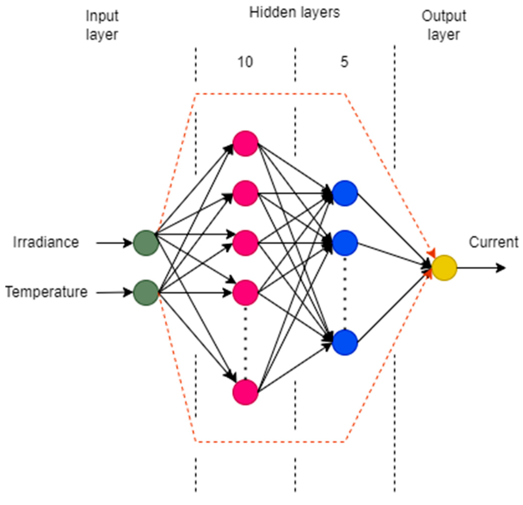
Cascade forward neural network (CFNN): analogous to a feedforward neural network; a cascading neural network interlinks the input and each preceding layer with the subsequent levels. For our model, this network was designed with a learning rate of 0.01 and 1000 epochs with a two-layer vector of 10 and 5 neurons forming the hidden layer.

(3)

General regression neural network (GRNN): a probabilistic network that employs regression when the output variable is continuous. The hidden layer consists of two components: the first calculates the Euclidean distance between the samples and the neuron’s ideal point, subsequently applying the RBF kernel function. The output is then transmitted to the second component, which has two neurons: the summation for the denominator and the units for the numerator. The denominator summation unit aggregates the weights of values from each hidden neuron, whereas the summation unit from the numerator computes the weights’ values multiplied by the target value for each hidden neuron. The output is given by the division of the denominator from the numerator unit [6]. For our model, the MATLAB function “newgrnn” will be used.

(4)

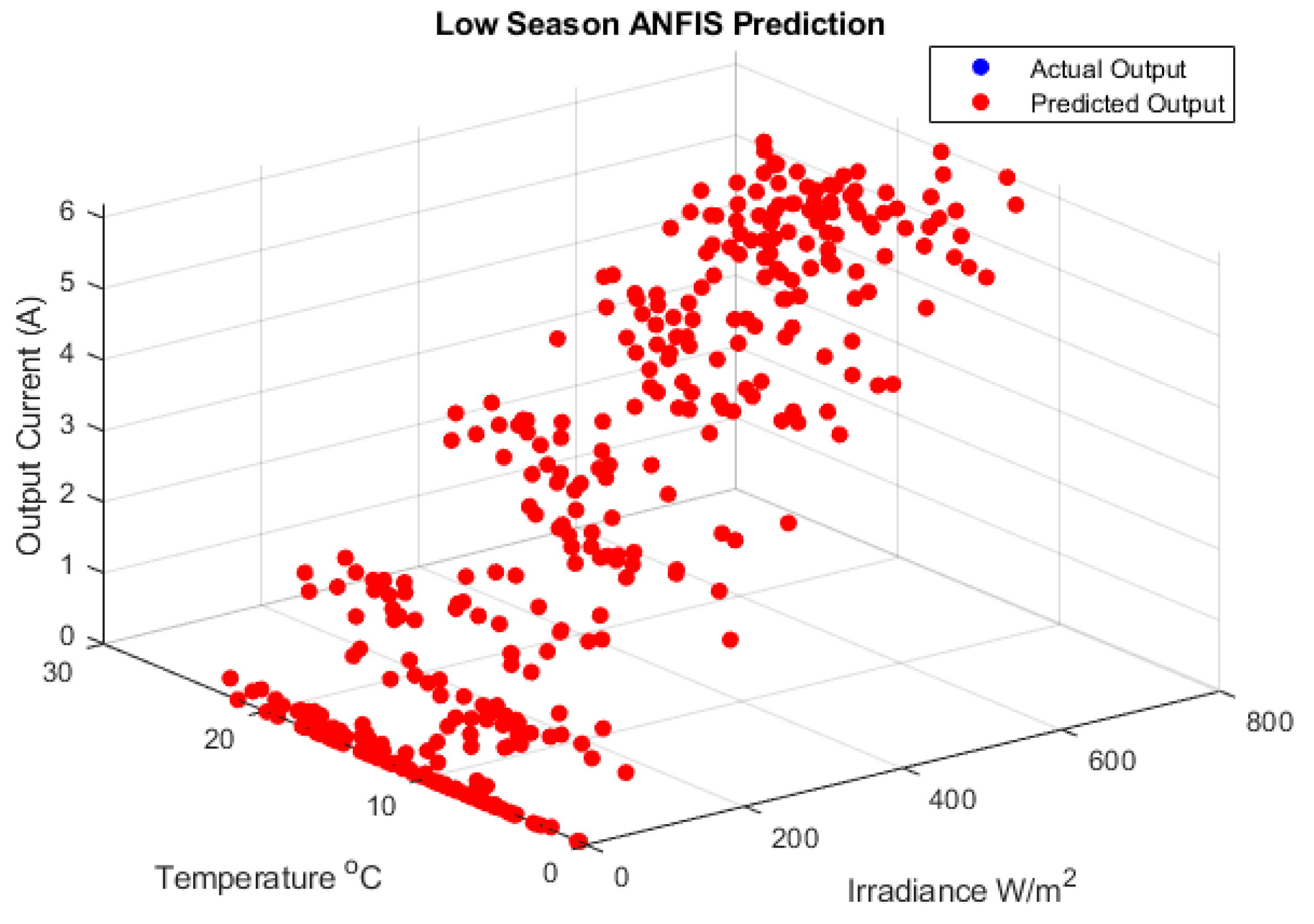
Adaptive neural fuzzy inference system (ANFIS): indicates a neural network that utilizes fuzzy inference methodology from Takagi–Sugeno. It is a unified framework that combines the benefits of fuzzy logic and neural networks, and it is equipped with a fuzzy inference system that is capable of learning. The neural network architecture consists of five layers: input, rule, normalization, consequent and output layers. In the input layer, inputs are fuzzified in accordance with premise parameters and membership functions (MFs). In the subsequent layer, neural nodes utilize a linear approach to evaluate the contributions of rules, utilizing parameters known as consequent parameters [32,33]. Our model used two inputs $x_1$ and $x_2$ with a single output $y$; the mathematical model of the algorithm is given by the Equations (7)–(11):

$$O_{1,i}=\left\{\begin{array}{c}{\mu }_{A_i}\left(x_1\right), i=1, 2\\ {\mu }_{B_{i-2}}\left(x_2\right), i=3, 4\end{array}\right.$$

(7)

$$O_{2,i}=w_i={\mu }_{A_i}\left(x_1\right){\mu }_{B_i}\left(x_2\right) i=1,2$$

(8)

$$O_{3,i}=\overline{w_i}={\displaystyle \frac{w_i}{w_1+w_2}} i=1,2$$

(9)

$$O_{4,i}=\overline{w_i}{f}_i=\overline{w_i}\left(q_i{x}_1+r_i{x}_2+s_i\right) i=1,2$$

(10)

$$y={\displaystyle {\sum }_i}\left(\overline{w_i}{f}_i\right)={\displaystyle \frac{{\sum }_i\left(\overline{w_i}{f}_i\right)}{{\sum }_i{w}_i}} i=1,2$$

(11)

where $i$ defines the number of rules, and the outputs of the five layers are given by $O_{1,i}$, $O_{2,i}$, $O_{3,i}$, $O_{4,i}$ and $y$. Meanwhile $q_i$, $r_i$ and $s_i$ represent the consequent parameters, the consequent function is $f_i$, and the membership functions of type “gaussian” are ${\mu }_{A_i}$ and ${\mu }_{B_i}$. Figure 6 depicts the diagram of our chosen ANFIS method.

A map is provided in Figure 7 to display the different geolocations of the stations where the data were extracted.

3.3. Particle Swarm Optimization (PSO)

Particle swarm optimization is an algorithm that uses metaheuristics grounded in the principles of swarm intelligence, drawing inspiration from the social behaviors exhibited by groups of animals, such as birds or fish. A swarm is a population where each member is called a particle and is a potential solution to the optimization problem and is randomly iterating its position following a velocity vector while keeping track of its best personal position and the best global positions of the swarm [34,35]. The Equations (12) and (13) determine the velocity and the position of a particle as they are updated during iterations:

$$V_{t+1}=w{V}_t+r_1{c}_1\left(P_t-X_t\right)+r_2{c}_2(G_t-X_t)$$

(12)

$$X_{t+1}=X_t+V_{t+1}$$

(13)

where $w$ is the inertia weight, $r_1$ and $r_2$ are random integers within the range of 0 to 1, and $c_1$ and $c_2$ are the acceleration constants. $P_t$ and $G_t$ are the best personal and global positions at iteration $t$. The objective function is obtained by minimization of the root mean square error of the weighted links of each ANN model. Figure 8 depicts a particle’s vector position diagram.

4. Results and Discussion

4.1. Models Evaluation Metrics

From Figure 9, the monthly variations in temperatures and solar radiations in our targeted regions clearly depict that the months of May, June and July comprise the low seasons (LS) in term of solar radiation; meanwhile, the months of November, December and January comprise the high season (HS) of solar radiations throughout the year. These periods will allow us to describe the behavior of our algorithms. For the two periods (LS and HS), the extracted data were partitioned into 70% for training and 30% for testing for each method which means for a pool of 1288 data, there are 902 units for training and 386 units for testing for each period and each algorithm.

The statistical results in

Table 2. Low-season prediction results.

	Low-Season Prediction Accuracy
	CSIR			Johannesburg			Pretoria			Vuwani			Zululand
ANN Techniques	RMSE	MAPE	MBE	RMSE	MAPE	MBE	RMSE	MAPE	MBE	RMSE	MAPE	MBE	RMSE	MAPE	MBE
GRNN	0.0136828	$2.23\times {10}^2$	$-1.35\times {10}^{-4}$	0.0127474	$-4.34\times {10}^{-6}$	$1.02\times {10}^{-4}$	0.0150858	−0.6351235	$-1.38\times {10}^{-4}$	0.0124866	1.2645113	$1.55\times {10}^{-4}$	0.0089106	6.252087	$-5.07\times {10}^{-4}$
FFNN	$5.98\times {10}^{-5}$	1.4469818	$-8.99\times {10}^{-6}$	$1.08\times {10}^{-4}$	$-3.82\times {10}^{-5}$	$-2.66\times {10}^{-5}$	$2.32\times {10}^{-4}$	−0.0462752	$2.31\times {10}^{-5}$	$3.42\times {10}^{-5}$	−0.0232012	$-2.34\times {10}^{-6}$	$1.85\times {10}^{-5}$	0.0132306	$7.38\times {10}^{-8}$
CFNN	$3\times {10}^{-8}$	$3.30\times {10}^{-5}$	$-3.36\times {10}^{-9}$	$1.81\times {10}^{-7}$	−0.03484	$-4.27\times {10}^{-8}$	0.0028605	0.0039847	$2.35\times {10}^{-4}$	$6.11\times {10}^{-7}$	$-4.43\times {10}^{-5}$	$1\times {10}^{-7}$	$3.03\times {10}^{-8}$	$4.06\times {10}^{-7}$	$5.12\times {10}^{-10}$
ANFIS	$1\times {10}^{-8}$	$3.16\times {10}^{-5}$	$1.33\times {10}^{-9}$	$1.77\times {10}^{-8}$	−2.048241	$4.38\times {10}^{-9}$	$2.75\times {10}^{-8}$	$-4.21\times {10}^{-6}$	$8.15\times {10}^{-9}$	$1.97\times {10}^{-8}$	$-5.85\times {10}^{-6}$	$6.60\times {10}^{-9}$	$1.42\times {10}^{-8}$	$-6.22\times {10}^{-6}$	$3.88\times {10}^{-10}$

demonstrate that in poor weather conditions, the best performing algorithm throughout the five cities is the adaptive neural fuzzy inference system (ANFIS) with the statistical metric of RMSE exhibiting values of $1.00\times {10}^{-8}$ in CSIR, $1.77\times {10}^{-8}$ in Johannesburg, $2.75\times {10}^{-8}$ in Pretoria, $1.97\times {10}^{-8}$ in Vuwani and $1.42\times {10}^{-8}$ in Zululand. Figure 10 and Figure 11 depict the training error of the ANFIS algorithm in the CSIR region and the scatter plot of the actual data given by the empirical formula against the forecasted data.

The training error converges from $4.1611\times {10}^{-9}$ to $-1$ while the algorithm was initialized with the gaussian membership function with two membership functions (MFs) and four rules. The function iterated through 100 epochs with the error goal set at $1\times {10}^{-4}$.

However,

Table 3. High-season prediction results.

	High-Season Prediction Accuracy
	CSIR			Johannesburg			Pretoria			Vuwani			Zululand
ANN Techniques	RMSE	MAPE	MBE	RMSE	MAPE	MBE	RMSE	MAPE	MBE	RMSE	MAPE	MBE	RMSE	MAPE	MBE
GRNN	0.0149624	1.1584395	−0.0010301	$1.35\times {10}^{-2}$	1.1478856	$1.35\times {10}^{-4}$	0.0140996	1.048151	$2.36\times {10}^{-4}$	0.0152396	1.3242254	$-5.02\times {10}^{-4}$	0.0112084	1.1594524	$9.28\times {10}^{-5}$
FFNN	$5.42\times {10}^{-5}$	0.0074414	$-6.06\times {10}^{-6}$	$6.38\times {10}^{-5}$	0.0298285	$-1.28\times {10}^{-6}$	$1.87\times {10}^{-5}$	0.0037762	$2.15\times {10}^{-6}$	$2.77\times {10}^{-7}$	$6.60\times {10}^{-5}$	$1.44\times {10}^{-9}$	$5.36\times {10}^{-5}$	0.0216027	$-3.22\times {10}^{-7}$
CFNN	$2.05\times {10}^{-11}$	$2.48\times {10}^{-9}$	$-1.11\times {10}^{-12}$	$2.49\times {10}^{-9}$	$1.39\times {10}^{-6}$	$6.92\times {10}^{-10}$	$2.28\times {10}^{-10}$	$5.55\times {10}^{-8}$	$-1.41\times {10}^{-10}$	$5.75\times {10}^{-10}$	$4.91\times {10}^{-8}$	$5.10\times {10}^{-12}$	$2.59\times {10}^{-14}$	$6.92\times {10}^{-12}$	$-1.36\times {10}^{-15}$
ANFIS	$3.79\times {10}^{-9}$	$2.79\times {10}^{-7}$	$-8.82\times {10}^{-10}$	$2.38\times {10}^{-9}$	$5.02\times {10}^{-7}$	$1.02\times {10}^{-10}$	$2.91\times {10}^{-9}$	$4.30\times {10}^{-7}$	$1.30\times {10}^{-10}$	$3.06\times {10}^{-9}$	$3.67\times {10}^{-7}$	$-2.61\times {10}^{-10}$	$1.99\times {10}^{-8}$	$1.64\times {10}^{-6}$	$-1.19\times {10}^{-8}$

displays the statistical metrics in better weather conditions. The best accuracy performance throughout the cities is given by the cascade feedforward neural network (CFNN) with RMSE metrics of $2.05\times {10}^{-11}$ in CSIR, $2.49\times {10}^{-9}$ in Johannesburg, $2.28\times {10}^{-10}$ in Pretoria, $5.75\times {10}^{-10}$ in Vuwani and $2.59\times {10}^{-14}$ in Zululand. Figure 12 shows the structure of the CFNN with two inputs for irradiance and temperature, two hidden layers made of 10 and 5 neurons and the interconnections to the output layer.

Figure 13 display the best performance for mean square error which is validated at the 6th epoch with a value of $2.3243\times {10}^{-24}$. Meanwhile, Figure 14 shows the regression plot which has an outstanding correlation coefficient R with a value of 1 for training, validation and testing performances. The scatter plot in Figure 15 shows the prediction results compared to the actual data in the region of Zululand. The scatter plot shows how the predicted data fit with great precision to the actual data in contrast with the GRNN scatter plot prediction in Figure 16 which reveals the inefficiency of the method to meet the expected data points.

Figure 17 and Figure 18 display six-day prediction traces from the four algorithms in CSIR and Zululand. Due to the high resolution of the prediction accuracy from the algorithms, it is difficult to perceive the differences between the traces compared to the actual data trace. However, Figure 19 provides a zoomed view of the traces in CSIR at hour number 16.

4.2. Models Optimization

The process of developing an optimization model consists of five parts. The first step is to collect data. Second, identify and define the problem to be solved, also called the problem function. Third, create a model based on the problem. Fourth, validate the model and evaluate its performance, and last, interpret the results [34]. The main objective of PSO during the models’ optimization process is to find the optimum weights and bias of the neural network before the training process; this is accomplished by determining the MSE during the iteration of every particle in the swarm. Depending on the swarm’s population, every iteration will determine the particle’s personal and global best position. Then, the neural network will be updated with the best global positions of their optimum weights and bias; Figure 20 depicts the general optimization process of our models.

The optimization process was conducted during the low season for the CSIR region. The selected parameter for the swarm population is 50 with a maximum iteration of 100. The inertia weight (w) is 0.7 while the cognitive (c₁) and social (c₂) learning coefficients were both 1.5.

Table 4. Comparison of optimization metrics.

	Low-Season CSIR
	No Optimization			PSO Optimization
ANN	RMSE	MAPE %	MBE	RMSE	MAPE %	MBE
GRNN	0.013683	$2.23\times {10}^2$	$-1.35\times {10}^{-4}$	0.331959	$6.67\times {10}^3$	$-7.64\times {10}^{-2}$
FFNN	$5.98\times {10}^{-5}$	1.446982	$-8.99\times {10}^{-6}$	$3\times {10}^{-5}$	0.127311	$-1.05\times {10}^{-6}$
CFNN	$3\times {10}^{-8}$	$3.30\times {10}^{-5}$	$-3.36\times {10}^{-9}$	$5.28\times {10}^{-14}$	$1.66\times {10}^{-9}$	$-8.21\times {10}^{-15}$
ANFIS	$1\times {10}^{-8}$	$3.16\times {10}^{-5}$	$1.33\times {10}^{-9}$	$9.15\times {10}^{-9}$	$8.34\times {10}^{-5}$	$7.07\times {10}^{-10}$

demonstrates a significant improvement in the statistical metrics of MSE, MBE and MAPE for all the models. For RMSE only, ANFIS improves from $1.00\times {10}^{-8}$ to $9.15\times {10}^{-9}$, from $3.00\times {10}^{-8}$ to $5.28\times {10}^{-14}$ for CFNN, from $5.98\times {10}^{-5}$ to $3\times {10}^{-5}$ for FFNN and from $0.0136$ to $0.3319$ for GRNN, which describes the general impact of our optimizer.

Figure 21 demonstrates that the best validation performance for the CFNN after optimization is given at epoch 7 with a mean squared error (MSE) of $4.6111\times {10}^{-28}$ which show a clear difference from Figure 13 before optimization.

5. Conclusions

This paper presented a comparative analysis between four ANN algorithms, namely ANFIS, CFNN, FFNN and GRNN, for forecasting PV output current. The analysis was conducted in five regions in South Africa during the best and poorest irradiation seasons. The outputs revealed that the ANFIS algorithm presented the best performances in poor seasons throughout the regions with the lowest value for RMSE of 1.00 × 10⁻⁸ in CSIR. Meanwhile, the CFNN technique was superior in better weather conditions with the lowest value of RMSE estimated at 2.05 × 10⁻¹¹ in the CSIR, and the GRNN technique presented the least accurate prediction in all regions. Applying particle swarm optimization generally improved the accuracy of the different techniques except for the GRNN.

Although our model for optimizing the different algorithms has an impact on prediction accuracy performance, it also presented some limitations which could be addressed by using hybrid optimizer approaches such as PSO-GA or PSO-ant colony optimizations; performance improvement could also be found in the selection of metaheuristic parameters.

The model presented could be used in many applications such as maximum power point tracking and any application where maximum accuracy is required.

References

1. Kanhukamwe, F.N. Matching Renewable Energy to the South African Electricity System. Master’s Thesis, Stellenbosch University, Stellenbosch, South Africa, 2019. [Google Scholar]
2. Sahu, B.K. A study on global solar PV energy developments and policies with special focus on the top ten solar PV power producing countries. Renew. Sustain. Energy Rev. 2015, 43, 621–634. [Google Scholar] [CrossRef]
3. Foley, A.; Olabi, A.G. Renewable energy technology developments, trends and policy implications that can underpin the drive for global climate change. Renew. Sustain. Energy Rev. 2017, 68, 1112–1114. [Google Scholar] [CrossRef]
4. Li, G.; Xie, S.; Wang, B.; Xin, J.; Li, Y.; Du, S. Photovoltaic power forecasting with a hybrid deep learning approach. IEEE Access 2020, 8, 175871–175880. [Google Scholar] [CrossRef]
5. Antonanzas, J.; Osorio, N.; Escobar, R.; Urraca, R.; Martinez-de-Pison, F.J.; Antonanzas-Torres, F. Review of photovoltaic power forecasting. Sol. Energy 2016, 136, 78–111. [Google Scholar] [CrossRef]
6. Khatib, T.; Elmenreich, W. Modeling of Photovoltaic Systems Using MATLAB®: Simplified Green Codes; John Wiley & Sons: Hoboken, NJ, USA, 2016. [Google Scholar]
7. Bukhari, M.M.; Alkhamees, B.F.; Hussain, S.; Gumaei, A.; Assiri, A.; Ullah, S.S. An improved artificial neural network model for effective diabetes prediction. Complexity 2021, 2021, 5525271. [Google Scholar] [CrossRef]
8. Panda, M.M.; Panda, S.N.; Pattnaik, P.K. Exchange rate prediction using ANN and deep learning methodologies: A systematic review. In Proceedings of the 2020 Indo–Taiwan 2nd International Conference on Computing, Analytics and Networks (Indo-Taiwan ICAN), Rajpura, India, 7–15 February 2020; pp. 86–90. [Google Scholar]
9. Xiang, Z.; Magnini, V.P.; Fesenmaier, D.R. Information technology and consumer behavior in travel and tourism: Insights from travel planning using the internet. J. Retail. Consum. Serv. 2015, 22, 244–249. [Google Scholar] [CrossRef]
10. Arora, A.; Gupta, M.; Mehmi, S.; Khanna, T.; Chopra, G.; Kaur, R.; Vats, P. Towards Intelligent Governance: The Role of AI in Policymaking and Decision Support for E-Governance. In Proceedings of the World Conference on Information Systems for Business Management, Bangkok, Thailand, 7–8 September 2023; pp. 229–240. [Google Scholar]
11. Jha, R. Review of Data Mining and Data Warehousing Implementation in E-Governance. Int. J. Innov. Sci. Res. Technol. (IJISRT) 2020, 5, 18–28. [Google Scholar] [CrossRef]
12. Li, X.; Sun, Y. Application of RBF neural network optimal segmentation algorithm in credit rating. Neural Comput. Appl. 2021, 33, 8227–8235. [Google Scholar] [CrossRef]
13. Abdolrasol, M.G.M.; Hussain, S.M.S.; Ustun, T.S.; Sarker, M.R.; Hannan, M.A.; Mohamed, R.; Ali, J.A.; Mekhilef, S.; Milad, A. Artificial neural networks based optimization techniques: A review. Electronics 2021, 10, 2689. [Google Scholar] [CrossRef]
14. Abraham, A. Artificial neural networks. In Handbook of Measuring System Design; John Wiley & Sons, Ltd.: Hoboken, NJ, USA, 2005. [Google Scholar]
15. Zappone, A.; Di Renzo, M.; Debbah, M.; Lam, T.T.; Qian, X. Model-aided wireless artificial intelligence: Embedding expert knowledge in deep neural networks for wireless system optimization. IEEE Veh. Technol. Mag. 2019, 14, 60–69. [Google Scholar] [CrossRef]
16. Zazoum, B. Solar photovoltaic power prediction using different machine learning methods. Energy Rep. 2022, 8, 19–25. [Google Scholar] [CrossRef]
17. Tovar, M.; Robles, M.; Rashid, F. PV power prediction, using CNN-LSTM hybrid neural network model. Case of study: Temixco-Morelos, México. Energies 2020, 13, 6512. [Google Scholar] [CrossRef]
18. Kumar, P.M.; Saravanakumar, R.; Karthick, A.; Mohanavel, V. Artificial neural network-based output power prediction of grid-connected semitransparent photovoltaic system. Environ. Sci. Pollut. Res. 2022, 29, 10173–10182. [Google Scholar] [CrossRef]
19. Suresh, V.; Janik, P.; Rezmer, J.; Leonowicz, Z. Forecasting solar PV output using convolutional neural networks with a sliding window algorithm. Energies 2020, 13, 723. [Google Scholar] [CrossRef]
20. Alblawi, A.; Said, T.; Talaat, M.; Elkholy, M. PV solar power forecasting based on hybrid MFFNN-ALO. In Proceedings of the 2022 13th International Conference on Electrical Engineering (ICEENG), Cairo, Egypt, 29–31 March 2022; pp. 52–56. [Google Scholar]
21. Montoya, A.Y.; Mandal, P. Day-ahead and week-ahead solar PV power forecasting using deep learning neural networks. In Proceedings of the 2022 North American Power Symposium (NAPS), Salt Lake City, UT, USA, 9–11 October 2022; pp. 1–6. [Google Scholar]
22. Salam, S.S.A.; Petra, M.; Azad, A.K.; Sulthan, S.M.; Raj, V. A Comparative Study on Forecasting Solar Photovoltaic Power Generation Using Artificial Neural Networks. In Proceedings of the 2023 Innovations in Power and Advanced Computing Technologies (i-PACT), Kuala Lumpur, Malaysia, 8–10 December 2023; pp. 1–6. [Google Scholar]
23. Mahmudah, N.; Priyadi, A.; Budi, A.L.S.; Putri, V.L.B. Photovoltaic Power Forecasting Using Cascade Forward Neural Network Based on Levenberg-Marquardt Algorithm. In Proceedings of the 2021 IEEE international Conference in Power Engineering Application (ICPEA), Malaysia, 8–9 March 2021; pp. 115–120. [Google Scholar]
24. Lu, Z.; Wang, Z.; Ren, Y. Photovoltaic Power Regression Model Based on Gauss Boltzmann Machine. In Proceedings of the 2020 39th Chinese Control Conference (CCC), Shenyang, China, 27–29 July 2020; pp. 6117–6122. [Google Scholar]
25. Theocharides, S.; Makrides, G.; Livera, A.; Theristis, M.; Kaimakis, P.; Georghiou, G.E. Day-ahead photovoltaic power production forecasting methodology based on machine learning and statistical post-processing. Appl. Energy 2020, 268, 115023. [Google Scholar] [CrossRef]
26. Khan, I.; Zhu, H.; Khan, D.; Panjwani, M.K. Photovoltaic Power prediction by Cascade forward artificial neural network. In Proceedings of the 2017 International Conference on Information and Communication Technologies (ICICT), Karachi, Pakistan, 30–31 December 2017; pp. 145–149. [Google Scholar]
27. Ge, L.; Li, Y.; Xian, Y.; Wang, Y.; Liang, D.; Yan, J. A FA-GWO-GRNN method for short-term photovoltaic output prediction. In Proceedings of the 2020 IEEE Power & Energy Society General Meeting (PESGM), Montreal, QC, Canada, 2–6 August 2020; pp. 1–5. [Google Scholar]
28. Haque, A.U.; Nehrir, M.H.; Mandal, P. Solar PV power generation forecast using a hybrid intelligent approach. In Proceedings of the 2013 IEEE Power & Energy Society General Meeting, Vancouver, BC, Canada, 21–25 July 2013; pp. 1–5. [Google Scholar]
29. Singh, V.P.; Vijay, V.; Bhatt, M.S.; Chaturvedi, D. Generalized neural network methodology for short term solar power forecasting. In Proceedings of the 2013 13th International Conference on Environment and Electrical Engineering (EEEIC), Wroclaw, Poland, 1–3 November 2013; pp. 58–62. [Google Scholar]
30. Irmak, E.; Yesilbudak, M.; Tasdemir, O. Daily Prediction of PV Power Output Using Particulate Matter Parameter with Artificial Neural Networks. In Proceedings of the 2023 11th International Conference on Smart Grid (icSmartGrid), Paris, France, 4–7 June 2023; pp. 1–4. [Google Scholar]
31. Hack, S. Machine Learning: 2 Books in 1: An Introduction Math Guide for Beginners to Understand Data Science Through the Business Applications; Chopra International Consulting Limited: London, UK, 2020. [Google Scholar]
32. Halabi, L.M.; Mekhilef, S.; Hossain, M. Performance evaluation of hybrid adaptive neuro-fuzzy inference system models for predicting monthly global solar radiation. Appl. Energy 2018, 213, 247–261. [Google Scholar] [CrossRef]
33. Cheng, L.; Zang, H.; Ding, T.; Wang, M.; Wei, Z.; Sun, G. A combined optimization structure of adaptive neuro-fuzzy inference system for probabilistic photovoltaic power forecasting. In Proceedings of the 2019 IEEE Power & Energy Society General Meeting (PESGM), Atlanta, GA, USA, 4–8 August 2019; pp. 1–5. [Google Scholar]
34. Ansari, M.T.; Rizwan, M. ANN and PSO based Approach for Solar Energy Forecasting: A Step Towards Sustainable Power Generation. In Proceedings of the 2021 4th International Conference on Recent Developments in Control, Automation & Power Engineering (RDCAPE), Noida, India, 7–8 October 2021; pp. 413–417. [Google Scholar]
35. Eberhart, R.; Kennedy, J. A new optimizer using particle swarm theory. In Proceedings of the MHS’95. Proceedings of the Sixth International Symposium on Micro Machine and Human Science, Nagoya, Japan, 4–6 October 1995; pp. 39–43.
Figure 1. ANN architecture.
Forecasting 07 00001 g001
Figure 2. University of Pretoria station.
Forecasting 07 00001 g002
Figure 3. CSIR station.
Forecasting 07 00001 g003
Figure 4. Venda station.
Forecasting 07 00001 g004
Figure 5. Zululand university station.
Forecasting 07 00001 g005
Figure 6. ANFIS diagram.
Forecasting 07 00001 g006
Figure 7. SAURAN station’s locations.
Forecasting 07 00001 g007
Figure 8. PSO particle’s position diagram.
Forecasting 07 00001 g008
Figure 9. Monthly irradiance and temperature in 2023.
Forecasting 07 00001 g009
Figure 10. ANFIS training error in CSIR.
Forecasting 07 00001 g010
Figure 11. Poor-season ANFIS prediction.
Forecasting 07 00001 g011
Figure 12. CFNN architecture diagram.
Forecasting 07 00001 g012
Figure 13. CFNN best validation performance.
Forecasting 07 00001 g013
Figure 14. CFNN regression plot diagram.
Forecasting 07 00001 g014
Figure 15. High-season CFNN prediction.
Forecasting 07 00001 g015
Figure 16. High-season GRNN prediction.
Forecasting 07 00001 g016
Figure 17. Six-day prediction trace of the four methods in CSIR.
Forecasting 07 00001 g017
Figure 18. Six-day prediction traces of the four methods in Zululand.
Forecasting 07 00001 g018
Figure 19. A zoomed view of traces in CSIR.
Forecasting 07 00001 g019
Figure 20. PSO optimization process.
Forecasting 07 00001 g020
Figure 21. Optimized CFNN validation performance.
Forecasting 07 00001 g021