Article

Machine Learning-Enhanced Pairs Trading

1
Centro de Ciências Sociais Aplicadas, Universidade Presbiteriana Mackenzie, Rua da Consolação 930, Sao Paulo 01302-907, SP, Brazil
2
Courant Institute of Mathematical Sciences, New York University, 251 Mercer Street, New York, NY 10012, USA
3
University of Rochester, 500 Joseph C. Wilson Blvd, Rochester, NY 14627, USA
*
Author to whom correspondence should be addressed.
Forecasting 2024, 6(2), 434-455; https://doi.org/10.3390/forecast6020024
Submission received: 29 April 2024 / Revised: 1 June 2024 / Accepted: 4 June 2024 / Published: 11 June 2024
(This article belongs to the Special Issue Forecasting Financial Time Series during Turbulent Times)

Abstract

:
Forecasting returns in financial markets is notoriously challenging due to the resemblance of price changes to white noise. In this paper, we propose novel methods to address this challenge. Employing high-frequency Brazilian stock market data at one-minute granularity over a full year, we apply various statistical and machine learning algorithms, including Bidirectional Long Short-Term Memory (BiLSTM) with attention, Transformers, N-BEATS, N-HiTS, Convolutional Neural Networks (CNNs), and Temporal Convolutional Networks (TCNs) to predict changes in the price ratio of closely related stock pairs. Our findings indicate that a combination of reversion and machine learning-based forecasting methods yields the highest profit-per-trade. Additionally, by allowing the model to abstain from trading when the predicted magnitude of change is small, profits per trade can be further increased. Our proposed forecasting approach, utilizing a blend of methods, demonstrates superior accuracy compared to individual methods for high-frequency data.
JEL Classification:
C45; C53; C63; G12

1. Introduction

Pairs trading is the simultaneous purchase and sale of two closely related securities. The premise behind pairs trading is to capitalize on temporary divergences in the relative prices (spread) of two assets that are historically linked while remaining market neutral. An early example was developed by Bamberger and Tartaglia, at Morgan Stanley in the 1980s [1] that sought to exploit temporary deviations in the spread of two cointegrated assets.
According to [2], the procedure is based on a two-step sequence. The first is to find a pair of stocks, preferably from the same economic sector or from the same underlying asset (e.g., different classes of stocks for the same company), because such pairs often move in a coordinated fashion.
Having found two such stocks, say A and B, the idea of pairs trading is to short a certain value v of A and to long value v of B with the hope that stock B will rise relative to stock A over some time period, after which the positions would be liquidated. If the ratio of the two stock prices is r, i.e.,
r · price B = price A
then this would entail buying r shares of B for every share of A sold.
Pairs trading is an example of high-frequency trading. Such trading is a prominent feature in today’s financial markets, and contributes to a significant portion of total equity trading, as noted in [3,4]. Ref. [5] states that high-frequency trading creates a two-tiered market, where fast traders mostly deal with each other, leaving slower investors with less profitable deals. Studies such as [6,7] have indicated that high-frequency pairs trading strategies can demonstrate statistically significant average excess returns.
The challenges of implementing pairs trading in a high-frequency trading strategy include:
  • Data availability: Pairs trading relies on identifying correlated or co-integrated securities, which requires access to accurate and timely data. Obtaining and processing this data in real-time can be challenging.
  • Execution speed: High-frequency trading requires rapid execution of trades, and delays in executing the pairs trading strategy can result in missed opportunities.
  • Transaction costs: High-frequency trading involves frequent trading, which can lead to higher transaction costs as shown by [8]. Such costs can negate the potential profits of pairs trading, suggesting that low-profit trades should be avoided.
This paper’s contributions are to identify a class of online adaptive hybrid pairs trading strategies that combine reversion, machine learning, and thresholding. As far as we can tell, there are no better algorithms available.

A Brief History of Forecasting for Finance

Ref. [9] showed that traditional econometric methods, such as Linear Regression, based on parametric assumptions, are effective when relationships between variables are linear and well-understood. In general, classical econometric methods also offer benefits such as interpretability and therefore insights into the economic mechanisms underlying data.
According to [10], methods like Autoregressive Integrated Moving Average (ARIMA) are commonly used for modeling time series data, such as financial market prices. Prices are notably easier to model than changes in prices. For example, a stock whose price varies around USD 100 for a year is well predicted by the single value of USD 100, but predicting the minute-by-minute changes is much more challenging.
Ensemble methods like Random Forests and Gradient Boosting Machines (GBMs) excel in handling large datasets and non-linear relationships, as indicated by [11]. These sophisticated machine learning methods are known for their flexibility in handling complex, high-dimensional data and for their ability to capture intricate patterns that may be missed by classical econometric methods. Deep learning methods [12] are often better than both econometric methods and random forest methods thanks to their ability to automatically learn representations from data, thereby enabling them to capture complex patterns and relationships.
A combination of machine learning and econometric techniques (e.g., random forests and linear regression), through ensemble methods can benefit from the strengths of each approach. The combination often involves crafting features based on economic theory and then applying machine learning algorithms to exploit complex patterns within those features and aims to mitigate the weaknesses of individual methods while maximizing their strengths, potentially leading to improved forecasting accuracy and profitability [13,14].
In both machine learning and econometric approaches, incorporating thresholds can avoid trading when there is substantial uncertainty [15].

2. Literature Review

2.1. Neural Network Techniques

Because neural networks have shown excellent performance in forecasting time series [16,17,18], we review them in this section and compare them in our experiments. Neural network models do not embody closed form modeling equations. Instead, they achieve their capabilities thanks to their architectures. We explain some important aspects of their architectures here below.
Long Short-Term Memory (LSTM): Introduced by [19], LSTM is an advanced variant of recurrent neural networks (RNNs) [20], which possess an internal architecture that includes memory gates, enabling them to maintain information from previous states and effectively capture temporal dependencies [19,21]. The memory gates in LSTMs regulate the flow of information within the cell state and allow the network to selectively remember or forget information over long periods [19], making them well-suited for time series data, because they can retain relevant information over extended sequences. The sequential module structure of LSTMs performs well compared to traditional methods [22,23,24,25]. Empirical research has shown that the Long Short-Term Memory (LSTM) is more accurate than traditional models in petroleum production predictions and in forecasting Chinese Stock Market returns [26,27].
Bidirectional LSTM (BiLSTM): A Bidirectional Long Short-Term Memory (BiLSTM) model is an advanced type of LSTM that can improve the understanding of context in time series data [28,29]. Unlike traditional LSTMs that process data in a forward direction, BiLSTMs analyze information in both forward and backward directions [29,30,31]. This forward and backward property of BiLSTMs allows them to use contextual information from both past and future time steps. Patterns in time series data, such as trends and seasonality, can be well learned by examining the data in both directions. BiLSTMs have particularly shown to be effective for complex time series forecasting tasks like power consumption prediction [31].
Transformers: Transformers, originally introduced for natural language processing tasks by [32], have been adapted for time series analysis, leveraging their ability to process sequences in parallel and capture long-range dependencies [32,33]. Unlike recurrent neural networks, transformers use self-attention mechanisms to weight the significance of different parts of the input data, allowing for the efficient and accurate modeling of time series [32,34,35]. In the context of time series, attention mechanisms in transformers identify the most relevant time steps, allowing the model to focus on significant patterns and dependencies across the entire sequence. By weighting the importance of different points in the time series, attention enables the model to capture intricate temporal dynamics. This architecture has shown significant promise in various time series applications, offering improvements in speed and accuracy over traditional methods [33,36,37].
N-BEATS: The N-BEATS model, proposed by [16] is a deep neural architecture based on backward and forward residual links and a very deep stack of fully connected layers [16]. N-BEATS is designed to be interpretable and modular, excelling in producing accurate forecasts and providing insights into the underlying patterns in the time series data [16]. It consists of sequential blocks where each block models trends as well as seasonality components through basis expansion layers. Each block refines its inputs using backcast outputs, which represent an approximation of the input window, allowing subsequent blocks to focus on the remaining unexplained patterns [16]. The forecast outputs from each block are accumulated to form the final prediction. The goal is that the model incrementally improves its accuracy [16]. This structure is effective for time series forecasting because it systematically decomposes and reconstructs the series, enhancing both predictive performance and interpretability. The model has outperformed the winning model of the M4 forecasting competition [16,17,18].
N-HiTS: N-HiTS is an advanced version of the N-BEATS model with a hierarchical architecture that captures temporal dynamics at multiple scales, crucial for diverse time series data [38]. N-HiTS’s hierarchical architecture decomposes the time series into multiple levels of granularity, allowing the model to capture patterns at different scales, which is helpful for accurately modeling complex temporal dynamics [38]. Additionally, the model leverages interpolation techniques to generate forecasts, helping to smooth and fill gaps in the data, making the predictions more robust and reliable [38]. This model is especially promising for long-term predictions in various fields, such as finance and weather forecasting [39].
Temporal Convolutional Network (TCN): Temporal Convolutional Networks (TCNs) make use of so-called causal convolutions, which are designed to ensure that the systems’ predictions are based solely on historical data [40,41,42]. These networks perform well in time series forecasting due to a few features. Causal convolutions ensure the output at time t depends only on inputs from time t and earlier, preserving the temporal order and preventing future data leakage [43]. TCNs achieve a large receptive field through a combination of dilated convolutions and deep networks, capturing long-term dependencies efficiently [40,41,43]. Residual connections, which skip layers, help mitigate the vanishing gradient problem and enable the training of very deep networks, enhancing the model’s ability to learn complex patterns [44]. TCNs have demonstrated superior performance over various contemporary machine learning models in tasks related to time series forecasting and classification [45,46,47]. In our experiments (see Section 7), they performed the best overall in terms of profit.

2.2. Strategies for Pairs Trading

Ref. [48] introduced the idea of doubly mean-reverting processes based on conditional modelling of model spreads between pairs of stocks. The strategy was designed to capture market inefficiencies with daily data. Results from real data back-testing showed high returns, even after subtracting transaction costs, with Sharpe ratios between 3.9 and 7.2.
Ref. [49] studied the Indian stock market using Volume Weighted Average Price (VWAP) to explore the possibility of making profits in intraday High-Frequency Trading. (To understand how VWAP is calculated, assume that 1000 shares trade at USD 50, 2000 shares at USD 48, and 5000 shares at USD 51, then the VWAP is ( 50 × 1000 ) + ( 48 × 2000 ) + ( 51 × 5000 ) 1000 + 2000 + 5000 . That is, multiply each price by volume and then divide by the sum of volumes.) The results indicate that various trader groups, using different strategies, can all achieve gains when engaging in liquidity-demanding trades.
Ref. [50], propose a Generalized Smooth Transition–Vector Error Correction Model, GST-VECM, to estimate the implied arbitrage mechanism from financial market data. Using Chinese financial markets data, the authors examine how the introduction of Exchange Traded Funds (ETF) affects index arbitrage on the Shanghai and Shenzen markets. Their model can be applied to any cointegrated financial time-series.
Ref. [51] propose a methodology for selecting candidate stock pairs for pairs trading based on the correlation between leads and lags of different time series. While our paper works with pairs that must be correlated because they come from the same underlying company, one could imagine using the methods of [51] and then applying our methods to trade.

3. Data Source

The data source for our work is the site [52], with millisecond resolution for the year 2022, using the trading platform robotrader [53]. The three companies chosen (Petrobras, Banco Itau, and Banco Bradesco) are highly visible in the main Brazilian stock exchange index Ibovespa because (i) they are among the most traded companies, (ii) they have high capitalization and (iii) they are highly sought after by all types of investors, both local and foreign. This implies they are difficult to manipulate.
The three companies’ stocks are not traded every millisecond however, creating gaps in the price time series. For that reason, we preprocessed the data by filling in the gaps using the last price traded. We further preprocessed the data by collapsing the trading summary into minutes, using the closing price of each minute in order to increase computational efficiency and reduce sensitivity to spurious fluctuations.
B3 [52] is Brazil’s stock exchange, from which the data used in this study are taken. The closing prices of the shares were obtained through the Robotrader trading platform, developed by [53], a subsidiary company of B3. Robotrader is a platform for electronic and algorithmic trading, developed for high-frequency trading on capital markets and financial derivatives.
The ratios we considered were from preferred and common stocks from each of the three companies as shown in Table 1. Thus we knew they were highly correlated. In fact, the Petrobas ordinary and preferred stocks had a price correlation of 0.98, the Banco Itau preferred and ordinary stocks had a correlation of 0.98 as well, and the Banco Bradesco pair had a correlation of 0.99.

4. Methodology

4.1. Experimental Framework

For each experiment on a pair of stocks, we used the first 50% of the sample to train the model (we compare the models later), 10% for validation, and 40% for testing. We implemented the following trading strategies.

4.1.1. Reversion Strategy

We choose the reversion strategy as a base method. Intuitively, this says that if the ratio at time t is greater than (resp. less than) the ratio at time t 1 , then it will go down (resp. go up) by time t + 1 . The decision making may be formalized as follows (with the A stock in the numerator of the ratios from the previous section):
Case 1: r t r t 1 > 0 = > sell A and buy B.
Case 2: r t r t 1 < 0 = > buy A and sell B.
Case 3: r t r t 1 = 0 = > do not trade.
Here, the third scenario acts as a guard against making trades when the difference between ratios is not conclusive by itself.

4.1.2. Pure Forecasting Strategy

This strategy trades solely based on the difference between the actual ratio at the current timestamp and the predicted ratio for the next (based on one of the forecasting strategies among those tested). It can be formalized as follows:
Case 1: p r e d t + 1 r t > 0 = > buy A and sell B.
Case 2: p r e d t + 1 r t < 0 = > sell A and buy B.
Case 3: p r e d t + 1 r t = 0 = > do not trade.
While the third scenario is extremely unlikely, we make it a point to include the “equal to zero” check. This helps in conservatively avoiding a trade when our model either accurately predicts no change in the ratio, or fails to capture the actual change. Later, we expand this third case to include a margin in which we do not trade if we are “close to zero”.

4.1.3. Hybrid Strategy

The profitability of each of the aforementioned strategies can be seen in the results section. In the hope of further improving the profit-per-trade, we have tried a hybrid strategy. As motivation, consider that reversion and pure forecasting end up making different trading decisions on many occasions. The hybrid strategy essentially aims to trade only when the reversion and pure-forecasting strategies agree. That is,
Case 1: p r e d t + 1 r t < 0 and r t r t 1 > 0 = > sell A and buy B.
Case 2: p r e d t + 1 r t > 0 and r t r t 1 < 0 = > buy A and sell B.
Case 3: In all other cases, do not trade.

4.2. Threshold Strategies

We test the concept of a “threshold strategy” to trade more conservatively. A threshold, in our case, is the least absolute difference in predicted ratio that is needed for a trade. The goal is to improve the overall profit-per-trade for the trades that take place for predictions that exceed the threshold.
Our experiments include two types of thresholds: static and dynamic. Static thresholds are pre-determined values which are independent of the data distribution and trading strategy. By contrast, dynamic thresholds are expressed as percentiles of the absolute ratio-change distribution. Since the ratios observed by the base and pure forecasting strategies are different, we generate a set of dynamic thresholds for each of them. The generation of these dynamic thresholds does not use the test data, which is sequestered during training and hyperparameter setting.

4.3. Evaluation Metrics

Sharpe Ratio:
The Sharpe Ratio (S), introduced by [54], is computed by dividing the excess return (average portfolio return minus risk-free rate) by the standard deviation of the returns, and provides a metric to assess the riskiness of a portfolio. The higher the Sharpe Ratio, the better is the risk-adjusted performance of a given portfolio, i.e., higher returns relative to the level of risk undertaken. In our case, because we are buying and selling the same amount on each initial trade, the risk-free return is 0. So the equation simplifies to
S = R ¯ p σ p
where:
S: Sharpe Ratio
R ¯ p : Average portfolio return
σ p : Standard deviation of portfolio returns
Accumulated Profit:
The accumulated profit metric is simply the running sum of the profits on the test set.
Profit-per-Trade:
This is the average of the profits per trade actually done. In other words, it is a ratio of the accumulated profit versus the total number of executed trades. This is a particularly useful metric when transaction costs are significant.
Confusion Matrix:
Since profitability is heavily influenced by the type of trade performed, one figure of merit of accuracy is a confusion matrix. Such matrices are often used to evaluate classification models, by computing the number of true positive, false positive, false negative, and true negative predictions. We follow a similar approach, where we treat the behavior of our strategy as a prediction of whether the ratio will increase or decrease at the next minute and evaluate the prediction against what happens as in Table 2. We lay out the confusion matrix as four numbers in a row as in Table 3. As we will see in Table 3, Table 4 and Table 5, the best forecasting method for accuracy is not the same as the best method for profit.

5. Model Training

5.1. Datasets

Based on the data described in Section 3, we derived three datasets:
1.
The “bbdc3_4” dataset encapsulates the ratio between the financial tickers bbdc3 (ordinary shares) and bbdc4 (preferred shares) from Banco Bradesco stocks.
2.
The “petr3_4” dataset encapsulates the ratio between the financial tickers petr4 (preferred shares) and petr3 (ordinary shares) from Petrobras stocks.
3.
The “itau3_4” dataset encapsulates the ratio between the financial tickers itau4 (preferred shares) and itau3 (ordinary shares) from Banco Itau stocks.

5.2. Training Methodology

As mentioned in Section 4.1, for each experiment on a pair of stocks, we used the first 50% of the sample to train the model, 10% for validation, and the last 40% for testing. None of the training or parameter tuning used the testing data.
We used the same training methodology for each machine learning model utilized in our study. All models were designed to process input data consisting of 50 time steps and predict the subsequent value. All the models use the Adam optimizer and are trained with a batch size of 1024 for 50 epochs with a learning rate of 0.0001. Furthermore, all the models are trained on a single V100 GPU on Google Colab. The loss function used for each model is mean squared error loss.
To find the optimal hyperparameter values for each machine learning method, we used the validation set for the bbdc3_4 dataset. Our methodology involved isolating each hyperparameter h, holding any previously set hyperparameters at their chosen values and other hyperparameters at their default values. We then incrementally increased the value of h. We continued incrementing as long as the Root Mean Squared Error decreased, signifying an improvement in performance. Upon observing an increase in RMSE, we chose the prior value for h. An exhaustive search of all combinations may have found better values, but our main purpose was to find good hyperparameter values in a uniform way across models and then to explore combinations with reversion and thresholds. As the reader will see below, the order of setting hyperparameters was in descending order of importance.
For instance, when using the BiLSTM with Attention model, we initially increased the number of layers in the BiLSTM while keeping the other aspects of the model constant. We continued increasing the number of layers as long as the RMSE decreased. Once the RMSE began to rise, we identified the previous number of layers as the optimal configuration. Subsequently, utilizing the optimal number of layers for the BiLSTM, we gradually increased the number of BiLSTM units in each layer while maintaining the rest of the model unchanged. Once again, we continued increasing the number of units as long as the RMSE decreased. This same method was applied to select the number of heads for the multi-head attention layer and the dimension of the dense layer. Here, the hyperparameters include the number of layers in the BiLSTM, the number of BiLSTM units in each layer, the number of heads for the multi-head attention layer, and the dimension of the dense layer.
The following outlines each model’s architecture along with the hyperparameter values found using the method above:
BiLSTM with Attention: The BiLSTM with attention model architecture incorporates bidirectional Long Short-Term Memory (BiLSTM) layers with attention mechanisms. The model consists of two layers of BiLSTM cells, each with 128 units, followed by a multi-head attention mechanism with 16 heads and a key dimension of 128. After the attention mechanism, the output undergoes global average pooling and global max pooling. The resulting pooled representations are concatenated and passed through a dense layer with 512 units and ReLU activation. Finally, a sigmoid activation function is applied to produce the model’s output. The hyperparameters were optimized in the following order: number of BiLSTM layers, number of units in the BiLSTM cells for each layer, number of multi-attention heads, dimension of the key, and dimension of the dense layer.
Vanilla Transformer: The transformer model architecture consists of a multi-head self-attention mechanism with four heads, operating on an embedding dimensionality of 256. The model comprises three encoder and three decoder layers, each with feed forward networks of dimension 16. Layer normalization without bias terms was applied for normalization, and a dropout rate of 0.2 was utilized for regularization. The hyperparameters were optimized in the following order: number of encoder and decoder layers, number of multi-attention heads, dimension of the embedding layer, dimension of feed forward network, type of layer normalization (between layer normalization with bias, layer normalization without bias, and RMS normalization), and dropout rate.
N-BEATS: The N-BEATS model architecture is composed of five layers organized into one block and two stacks. Each layer employs a feed forward network with a width of 512 units, and a dropout rate of 0.2 is applied for regularization. The hyperparameters were optimized in the following order: number of layers in each block, number of blocks in each stack, number of stacks, dimension of the feed forward network, and dropout rate.
N-HiTS: The model setup for the N-HiTS model is constructed with five layers organized into one block and two stacks. Each layer encompasses a feed forward network with a width of 512 units, and a dropout rate of 0.2 is employed for regularization. The hyperparameters were optimized in the following order: number of layers in each block, number of blocks in each stack, number of stacks, dimension of the feed forward network, and dropout rate.
Temporal Convolution Network (TCN): The model architecture for TCN utilizes a convolutional kernel size of 3 and consists of 8 layers, each with 64 filters. Dilation is applied with a base of 2, and weight normalization is enabled. A dropout rate of 0.2 is incorporated for regularization purposes. The hyperparameters were optimized in the following order: kernel size, number of filters, number of layers, dilation base, and dropout rate.
The performance of each model was evaluated using root mean squared error (RMSE), mean absolute scaled error (MASE), mean absolute percentage error (MAPE), and symmetric mean absolute percentage error (sMAPE). We used the Darts time series library in PyTorch [55] to implement and train these models.

6. Threshold-Dependent Hybrid Trading Algorithm

The full trading Algorithm 1 combines mean reversion with machine learning-based forecasting (e.g., temporal convolutional networks) and trades only if both exceed their respective thresholds: t h r e s h r e v e r s i o n and t h r e s h f o r e c a s t . Intuitively, the algorithm will trade only if both are “confident.” The forecasting and mean reversion thresholds are set statically or dynamically as described in Section 4.2.
The main trading loop in Algorithm 1 is called at each time point (e.g., a minute). The DETERMINE_TRADE routine uses the thresholds and the forecasts to decide whether to trade. EXECUTE_TRADE will trade if the action returned by DETERMINE_TRADE says so.
Algorithm 1 Threshold-Dependent Hybrid Trading Algorithm
1:
Define thresholds
2:
t h r e s h f o r e c a s t          ▹ Set the forecasting threshold either statically or dynamically
3:
t h r e s h r e v e r s i o n ▹ Set the mean reversion threshold either statically or dynamically
4:
 
5:
function determine_trade( p r e d t + 1 , r t , r t 1 )
6:
    Calculate differences
7:
     f o r e c a s t d i f f p r e d t + 1 r t
8:
     r e v e r s i o n d i f f r t r t 1
9:
 
10:
    if  f o r e c a s t d i f f < t h r e s h f o r e c a s t  and  r e v e r s i o n d i f f > t h r e s h r e v e r s i o n  then
11:
         a c t i o n  “sell A and buy B”
12:
    else if  f o r e c a s t d i f f > t h r e s h f o r e c a s t  and  r e v e r s i o n d i f f < t h r e s h r e v e r s i o n  then
13:
         a c t i o n  “buy A and sell B”
14:
    else
15:
         a c t i o n  “do not trade”
16:
    return  a c t i o n
17:
 
18:
Main loop running throughout the trading session
19:
while  t r a d i n g _ s e s s i o n _ i s _ a c t i v e   do
20:
     p r e d t + 1 g e t _ f o r e c a s t i n g _ p r e d i c t i o n ( ) ▹ Forecasted value for the next time point
21:
     r t g e t _ c u r r e n t _ r a t i o ( )                                                             ▹ Current ratio value
22:
     r t 1 g e t _ p r e v i o u s _ r a t i o ( )                                                      ▹ Previous ratio value
23:
     t r a d e _ a c t i o n determine_trade( p r e d t + 1 , r t , r t 1 )
24:
    execute_trade( t r a d e _ a c t i o n )                                      ▹ Execute trade based on action
25:
 
26:
End of trading session
27:
end_trading_session

7. Results

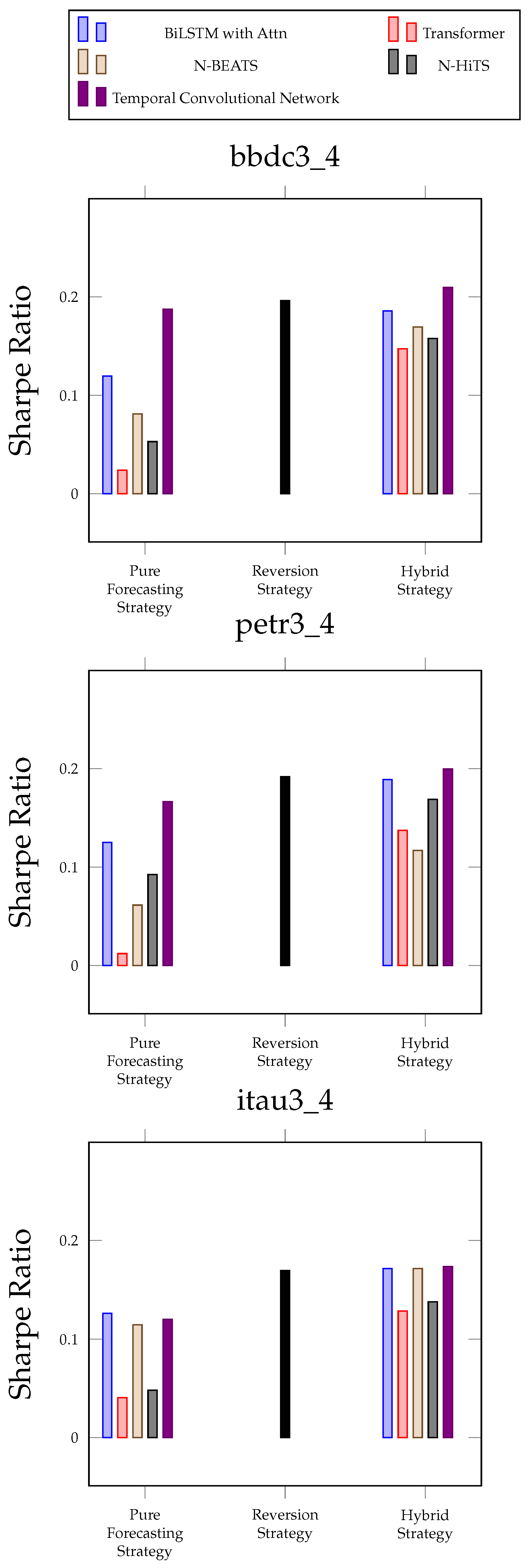
The tables and graphs in this section show that Temporal Convolutional Network is overall the best when it comes to profit (Figure 1) and profit-per-trade (Figure 2), but that the best models vary depending on the dataset when it comes to prediction error and accuracy (Table 3, Table 4 and Table 5). Regarding profit and the Sharpe ratio (Figure 3), the reversion strategy often beats all forecasting methods. A hybrid strategy using reversion with forecasting increases profit-per-trade relative to either by itself.

7.1. Threshold Experiments

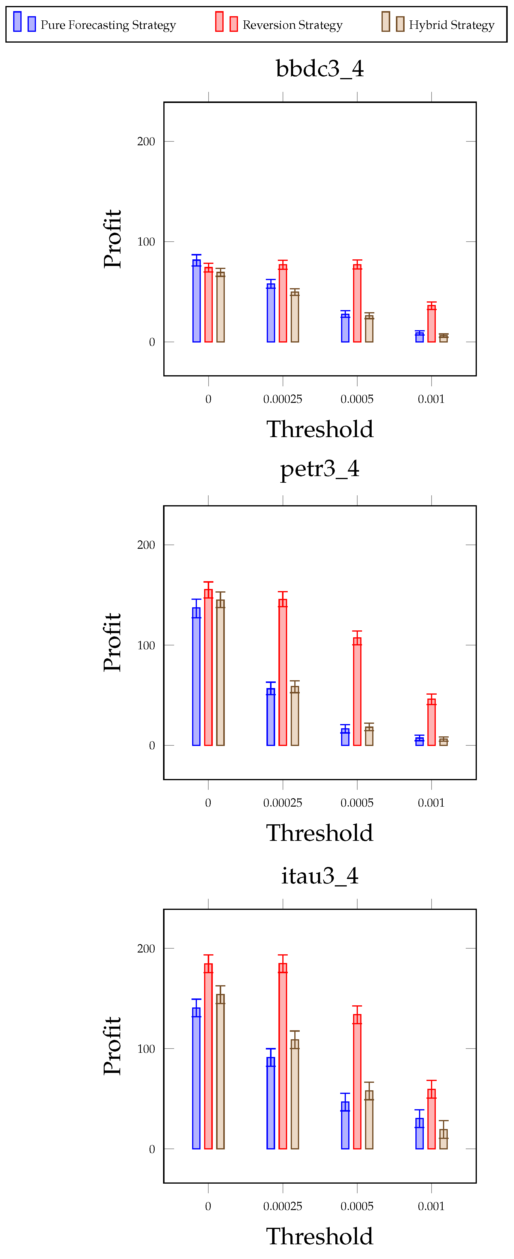
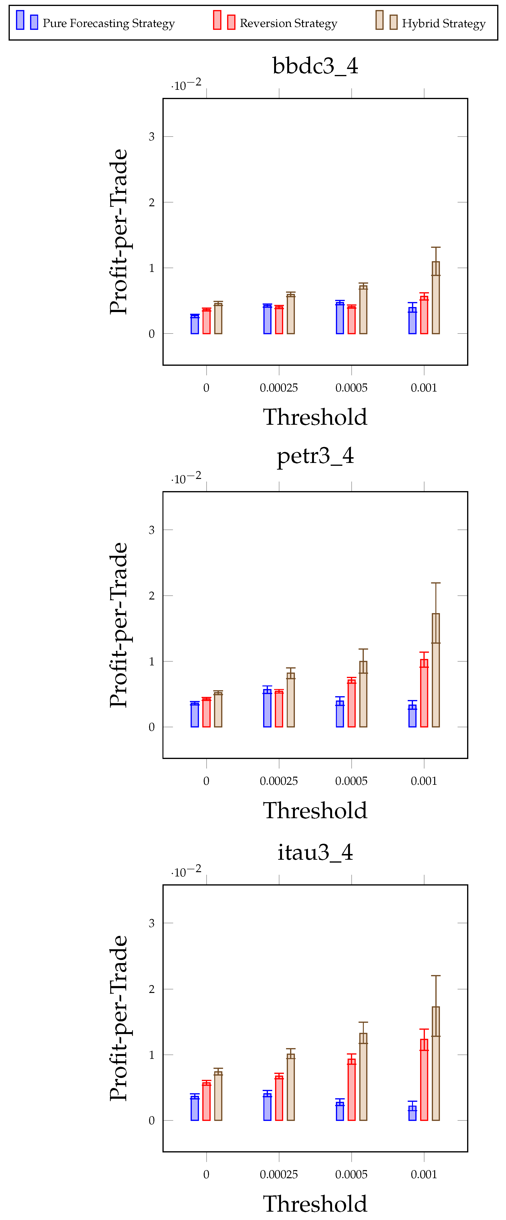
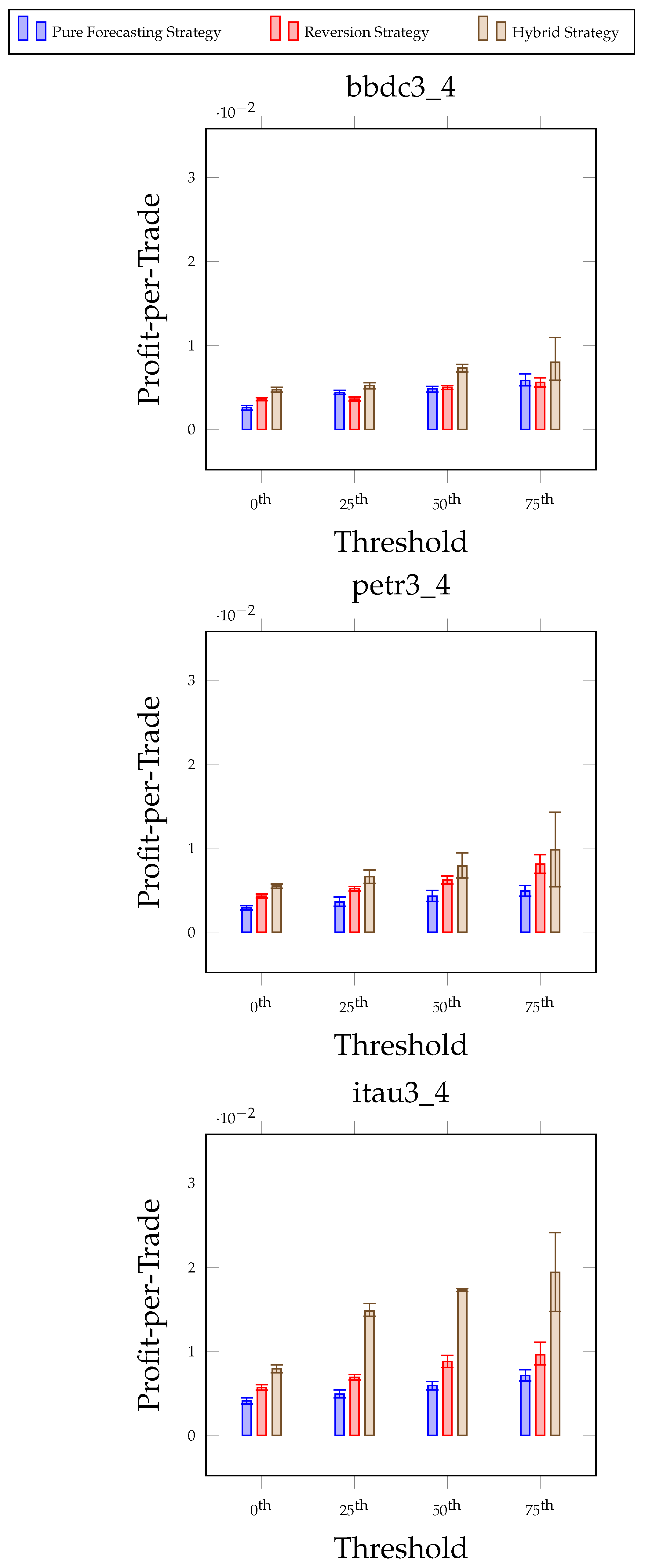
Because the Temporal Convolutional Network is overall the best forecasting method in terms of profit and profit-per-trade, we use it in the subsequent analysis whenever we refer to ‘Pure Forecasting Strategy’. The overall finding of this section is that thresholds improve profit-per-trade at the cost of trading less and therefore making less overall profit in a transaction cost-free environment. The Figure 4, Figure 5 and Figure 6, and Figure 7 illustrate these points for the case where there are no transaction costs (e.g. no brokerage fees).

7.2. Comparison with a Reinforcement Learning Approach

We performed a comparative analysis of our model with the reinforcement learning-based method [56] still ignoring transaction costs. The authors of that paper propose to enhance the pairs trading strategy through the use of a two-level reinforcement learning framework, where the Extended Option–Critic (EOC) [57] method is used for pair selection, and the Multi-Agent Deep Deterministic Policy Gradient (MADDPG) [58] method with three cooperating actors and one critic is used to set trading thresholds and execute trades. In our study, we re-implemented the MADDPG algorithm employed in their research to assess how it performs compared to our model (unfortunately, we were not able to obtain their code though we requested it). We did not need to use EOC in our comparison, because closely related stock pairs have already been selected in our study.
The key implementation details outlined in their paper include the following parameters: the buffer size (the memory capacity for experiences), the batch size (the number of experiences sampled from the buffer for each training iteration), gamma (the discount factor determining the importance of future rewards), the learning rate (the rate at which the model adjusts its parameters during training), the number of episodes (the number of complete runs through the training data), and the reward function (the metric used to evaluate the agent’s performance). In addition, they specified the set of variables describing the environment for both the actors (the decision-making components) and critic (the value function estimator), the action space (the possible actions the agent can take) for the actors, and the number of possible actions the actors could take. The paper specifies the values of these parameters.
We incorporated additional implementation details that were not explicitly outlined in the paper. The number of layers and number of neurons in each layer for the three actor and one critic neural networks were determined using the hyperparameter search discussed in Section 5.2 of this paper. The hyperparameters were optimized sequentially, beginning with the number of layers followed by the number of neurons in each layer. Each actor network comprises three fully connected layers, each with 64 neurons, followed by an output layer with neurons equal to the number of possible actions. The input to the network is the current state of the environment. The network employs the ReLU activation function for all hidden layers and utilizes the softmax function to produce a probability distribution over the available actions. The critic network, similar to the actor networks, consists of three fully connected layers, each with 64 neurons, followed by an output layer with a single neuron representing the quality of the actions taken by each actor. The input to the network is a combination of the current state and the actions taken by each actor. The network uses the ReLU activation function for all hidden layers.
Furthermore, we employed a tau value of 0.01 to update the target actor and critic networks. This tau value determines the rate at which the parameters of these target networks are updated, with a smaller tau resulting in a slower and more stable learning process. Additionally, we disabled exploration for the actors, focusing solely on exploiting learned policies. Lastly, we chose to train the networks using the Mean Squared Error (MSE) loss function.
Here are the results: The model was trained for 1000 time steps per episode, and the total profit we obtained on the test set was 29.7, which is nearly three times lower than the profit achieved using our approach.

7.3. Practical Implications of Experimental Results

Of the forecasting strategies, Temporal Convolutional Network performs the best in terms of profit, possibly because of its ability to capture both short-term and long-term dependencies with dilated convolutions. Reversion, however, often performs better than any forecasting strategy. Thresholds, whether dynamic or static, tend to reduce profits but increase profits per trade as well as the Sharpe ratio. Hybrid strategies also reduce profits but increase profits per trade.
It is possible that a reinforcement learning approach or another forecasting method or package such as Chronos [59] (which, at the time of writing, had just come out and did not perform well) might yield a better result than Temporal Convolutional Networks. Any better method can be drop-substituted for the Temporal Convolutional Network in our framework.
While the principal goal of our work is to study whether prediction in pairs trading is even possible, a fair question to ask is whether the strategy could make money in the face of brokerage fees. The minimum brokerage fee on the Brazilian stock market is around 0.011% of the monetary value of each intraday trade. Given this, we would need the average profit per trade to exceed that amount. Figure 8 shows that the hybrid strategy can make a profit-per-trade even when brokerage costs are taken into account. Moreover, when using a reasonably good threshold, the profit increases. These trends not only support our argument of using a hybrid strategy, but also justify the use of thresholds in reducing the number of loss-making trades.
As expected, the introduction of broker fees results in lower cumulative profits. Thresholds help substantially. Table 6 shows the observed profits for each strategy, when simulated with the highest dynamic threshold.

8. Conclusions

We were frankly surprised by the results we found. In spite of the fact that deltas in pair ratios resemble white noise, machine learning techniques such as temporal convolutional networks consistently generate profits in simulation. Further, the greater the magnitude of the predicted change in return does indeed correspond to a higher profit-per-trade, indicating that the machine learning based forecasting method tends to estimate magnitudes as well as directions correctly. Finally, hybridizing reversion with machine learning-based forecasting gives higher-quality predictions in terms of profit-per-trade than either method alone. This implies that machine learning is complementary to simple reversion. As machine learning methods improve, we foresee further improvements even for extremely difficult settings like these.
Code and pointers to public data will be available upon publication.

Author Contributions

Conceptualization: E.H. and D.S., Methodology: E.H., D.S., S.H. and B.L., Software: E.H., S.H. and B.L., Resources: E.H., Data Curation: E.H., Writing: E.H., D.S., S.H. and B.L., Supervision: D.S. All authors have read and agreed to the published version of the manuscript.

Funding

For this research, Eli Hadad Junior was supported by a scholarship from Capes/Print—Brazil. NYU Wireless also supported this work.

Institutional Review Board Statement

Not applicable.

Data Availability Statement

The software and data are available at https://github.com/bkmulusew/ml_pairs_trading (accessed on 10 March 2023).

Acknowledgments

We thank Mustafa Kocak for helpful comments.

Conflicts of Interest

The authors declare no conflict of interest.

References

  1. Bookstaber, R.M. A Demon of Our Own Design: Markets, Hedge Funds, and the Perils of Financial Innovation; John Wiley & Sons: Hoboken, NJ, USA, 2007. [Google Scholar] [CrossRef]
  2. Gatev, E.; Goetzmann, W.N.; Rouwenhorst, K.G. Pairs trading: Performance of a relative-value arbitrage rule. Rev. Financ. Stud. 2006, 19, 797–827. [Google Scholar] [CrossRef]
  3. Lhabitant, F.S.; Gregoriou, G.N. High-frequency trading: Past, present, and future. In Handbook of High Frequency Trading; Academic Press: San Diego, CA, USA, 2015; pp. 155–166. [Google Scholar] [CrossRef]
  4. Zaharudin, K.Z.; Young, M.R.; Hsu, W.H. High-frequency trading: Definition, implications, and controversies. J. Econ. Surv. 2022, 36, 75–107. [Google Scholar] [CrossRef]
  5. Virgilio, G. Is high-frequency trading tiering the financial markets? Res. Int. Bus. Financ. 2017, 41, 158–171. [Google Scholar] [CrossRef]
  6. Bogomolov, T. Pairs trading based on statistical variability of the spread process. Quant. Financ. 2013, 13, 1411–1430. [Google Scholar] [CrossRef]
  7. Krauss, C. Statistical arbitrage pairs trading strategies: Review and outlook. J. Econ. Surv. 2017, 31, 513–545. [Google Scholar] [CrossRef]
  8. Tokat, E.; Hayrullahoğlu, A.C. Pairs trading: Is it applicable to exchange-traded funds? Borsa Istanb. Rev. 2022, 22, 743–751. [Google Scholar] [CrossRef]
  9. Wooldridge, J.M. Introductory Econometrics: A Modern Approach; Nelson Education: Scarborough, ON, Canada, 2015. [Google Scholar]
  10. Box, G.E.; Jenkins, G.M.; Reinsel, G.C.; Ljung, G.M. Time Series Analysis: Forecasting and Control; John Wiley & Sons: Hoboken, NJ, USA, 2015. [Google Scholar] [CrossRef]
  11. Chen, T.; Guestrin, C. Xgboost: A scalable tree boosting system. In Proceedings of the 22nd ACM Sigkdd International Conference on Knowledge Discovery and Data Mining, San Francisco, CA, USA, 13–17 August 2016; pp. 785–794. [Google Scholar] [CrossRef]
  12. LeCun, Y.; Bengio, Y.; Hinton, G. Deep learning. Nature 2015, 521, 436–444. [Google Scholar] [CrossRef] [PubMed]
  13. Giudici, P. Applied Data Mining: Statistical Methods for Business and Industry; John Wiley & Sons: Hoboken, NJ, USA, 2005. [Google Scholar] [CrossRef]
  14. Shen, Y.; Khorasani, K. Hybrid multi-mode machine learning-based fault diagnosis strategies with application to aircraft gas turbine engines. Neural Netw. 2020, 130, 126–142. [Google Scholar] [CrossRef] [PubMed]
  15. Tsay, R.S. Analysis of Financial Time Series; John Wiley & Sons: Hoboken, NJ, USA, 2005. [Google Scholar] [CrossRef]
  16. Oreshkin, B.N.; Carpov, D.; Chapados, N.; Bengio, Y. N-BEATS: Neural basis expansion analysis for interpretable time series forecasting. arXiv 2019, arXiv:1905.10437. [Google Scholar] [CrossRef]
  17. Oreshkin, B.N.; Dudek, G.; Pełka, P.; Turkina, E. N-BEATS neural network for mid-term electricity load forecasting. Appl. Energy 2021, 293, 116918. [Google Scholar] [CrossRef]
  18. Makridakis, S.; Spiliotis, E.; Assimakopoulos, V. The M4 Competition: 100,000 time series and 61 forecasting methods. Int. J. Forecast. 2020, 36, 54–74. [Google Scholar] [CrossRef]
  19. Hochreiter, S.; Schmidhuber, J. Long Short-Term Memory. Neural Comput. 1997, 9, 1735–1780. [Google Scholar] [CrossRef] [PubMed]
  20. Elman, J.L. Finding Structure in Time. Cogn. Sci. 1990, 14, 179–211. [Google Scholar] [CrossRef]
  21. Gers, F.A.; Schmidhuber, J.; Cummins, F. Learning to Forget: Continual Prediction with LSTM. Neural Comput. 2000, 12, 2451–2471. [Google Scholar] [CrossRef] [PubMed]
  22. Malhotra, P.; Vig, L.; Shroff, G.M.; Agarwal, P. Long Short Term Memory Networks for Anomaly Detection in Time Series. In Proceedings of the European Symposium on Artificial Neural Networks, Bruges, Belgium, 22–24 April 2015. [Google Scholar]
  23. Karim, F.; Majumdar, S.; Darabi, H.; Chen, S. LSTM Fully Convolutional Networks for Time Series Classification. IEEE Access 2018, 6, 1662–1669. [Google Scholar] [CrossRef]
  24. Yunpeng, L.; Di, H.; Junpeng, B.; Yong, Q. Multi-step Ahead Time Series Forecasting for Different Data Patterns Based on LSTM Recurrent Neural Network. In Proceedings of the 2017 14th Web Information Systems and Applications Conference (WISA), Liuzhou, China, 11–12 November 2017; pp. 305–310. [Google Scholar] [CrossRef]
  25. Siami-Namini, S.; Tavakoli, N.; Siami Namin, A. A Comparison of ARIMA and LSTM in Forecasting Time Series. In Proceedings of the 2018 17th IEEE International Conference on Machine Learning and Applications (ICMLA), Orlando, FL, USA, 17–20 December 2018; pp. 1394–1401. [Google Scholar] [CrossRef]
  26. Sagheer, A.; Kotb, M. Time series forecasting of petroleum production using deep LSTM recurrent networks. Neurocomputing 2019, 323, 203–213. [Google Scholar] [CrossRef]
  27. Chen, K.; Zhou, Y.; Dai, F. A LSTM-based method for stock returns prediction: A case study of China stock market. In Proceedings of the 2015 IEEE International Conference on Big Data (Big Data), Santa Clara, CA, USA, 29 October–1 November 2015; pp. 2823–2824. [Google Scholar] [CrossRef]
  28. Schuster, M.; Paliwal, K. Bidirectional recurrent neural networks. IEEE Trans. Signal Process. 1997, 45, 2673–2681. [Google Scholar] [CrossRef]
  29. Graves, A.; Schmidhuber, J. Framewise phoneme classification with bidirectional LSTM and other neural network architectures. Neural Netw. 2005, 18, 602–610. [Google Scholar] [CrossRef] [PubMed]
  30. Siami-Namini, S.; Tavakoli, N.; Namin, A.S. The Performance of LSTM and BiLSTM in Forecasting Time Series. In Proceedings of the 2019 IEEE International Conference on Big Data (Big Data), Los Angeles, CA, USA, 9–12 December 2019; pp. 3285–3292. [Google Scholar] [CrossRef]
  31. da Silva, D.G.; de Moura Meneses, A.A. Comparing Long Short-Term Memory (LSTM) and bidirectional LSTM deep neural networks for power consumption prediction. Energy Rep. 2023, 10, 3315–3334. [Google Scholar] [CrossRef]
  32. Vaswani, A.; Shazeer, N.; Parmar, N.; Uszkoreit, J.; Jones, L.; Gomez, A.N.; Kaiser, Ł.; Polosukhin, I. Attention is all you need. arXiv 2017, arXiv:1706.03762. [Google Scholar] [CrossRef]
  33. Wen, Q.; Zhou, T.; Zhang, C.; Chen, W.; Ma, Z.; Yan, J.; Sun, L. Transformers in Time Series: A Survey. arXiv 2023, arXiv:2202.07125. [Google Scholar] [CrossRef]
  34. Wolf, T.; Debut, L.; Sanh, V.; Chaumond, J.; Delangue, C.; Moi, A.; Cistac, P.; Rault, T.; Louf, R.; Funtowicz, M.; et al. Transformers: State-of-the-Art Natural Language Processing. In Proceedings of the 2020 Conference on Empirical Methods in Natural Language Processing: System Demonstrations, Online, 16–20 November 2020; Liu, Q., Schlangen, D., Eds.; Association for Computational Linguistics: Stroudsburg, PA, USA, 2020; pp. 38–45. [Google Scholar] [CrossRef]
  35. Choi, H.; Cho, K.; Bengio, Y. Fine-grained attention mechanism for neural machine translation. Neurocomputing 2018, 284, 171–176. [Google Scholar] [CrossRef]
  36. Cholakov, R.; Kolev, T. Transformers predicting the future. Applying attention in next-frame and time series forecasting. arXiv arXiv:2108.08224. [CrossRef]
  37. Lim, B.; Arık, S.; Loeff, N.; Pfister, T. Temporal Fusion Transformers for interpretable multi-horizon time series forecasting. Int. J. Forecast. 2021, 37, 1748–1764. [Google Scholar] [CrossRef]
  38. Challu, C.; Olivares, K.G.; Oreshkin, B.N.; Ramirez, F.G.; Canseco, M.M.; Dubrawski, A. Nhits: Neural hierarchical interpolation for time series forecasting. Proc. AAAI Conf. Artif. Intell. 2023, 37, 6989–6997. [Google Scholar] [CrossRef]
  39. Benton, G.; Gruver, N.; Maddox, W.; Wilson, A.G. Deep Probabilistic Time Series Forecasting over Long Horizons. 2023. Available online: https://openreview.net/forum?id=22h1XSEiN0 (accessed on 10 March 2023).
  40. Lea, C.; Flynn, M.D.; Vidal, R.; Reiter, A.; Hager, G.D. Temporal convolutional networks for action segmentation and detection. In Proceedings of the IEEE Conference on Computer Vision and Pattern Recognition, Honolulu, HI, USA, 21–26 July 2017; pp. 156–165. [Google Scholar]
  41. Bai, S.; Kolter, J.Z.; Koltun, V. An empirical evaluation of generic convolutional and recurrent networks for sequence modeling. arXiv 2018, arXiv:1803.01271. [Google Scholar] [CrossRef]
  42. Wan, R.; Mei, S.; Wang, J.; Liu, M.; Yang, F. Multivariate Temporal Convolutional Network: A Deep Neural Networks Approach for Multivariate Time Series Forecasting. Electronics 2019, 8, 876. [Google Scholar] [CrossRef]
  43. van den Oord, A.; Dieleman, S.; Zen, H.; Simonyan, K.; Vinyals, O.; Graves, A.; Kalchbrenner, N.; Senior, A.; Kavukcuoglu, K. WaveNet: A Generative Model for Raw Audio. arXiv 2016, arXiv:1609.03499. [Google Scholar] [CrossRef]
  44. He, K.; Zhang, X.; Ren, S.; Sun, J. Deep Residual Learning for Image Recognition. arXiv 2015, arXiv:1512.03385. [Google Scholar] [CrossRef]
  45. Lara-Benítez, P.; Carranza-García, M.; Luna-Romera, J.M.; Riquelme, J.C. Temporal Convolutional Networks Applied to Energy-Related Time Series Forecasting. Appl. Sci. 2020, 10, 2322. [Google Scholar] [CrossRef]
  46. Koh, B.H.D.; Lim, C.L.P.; Rahimi, H.; Woo, W.L.; Gao, B. Deep Temporal Convolution Network for Time Series Classification. Sensors 2021, 21, 603. [Google Scholar] [CrossRef]
  47. Liu, Y.; Dong, H.; Wang, X.; Han, S. Time Series Prediction Based on Temporal Convolutional Network. In Proceedings of the 2019 IEEE/ACIS 18th International Conference on Computer and Information Science (ICIS), Beijing, China, 17–19 June 2019; pp. 300–305. [Google Scholar] [CrossRef]
  48. Liu, B.; Chang, L.B.; Geman, H. Intraday pairs trading strategies on high frequency data: The case of oil companies. Quant. Financ. 2017, 17, 87–100. [Google Scholar] [CrossRef]
  49. Arumugam, D. Algorithmic trading: Intraday profitability and trading behavior. Econ. Model. 2023, 128, 106521. [Google Scholar] [CrossRef]
  50. Chen, S.; Chng, M.T.; Liu, Q. The implied arbitrage mechanism in financial markets. J. Econom. 2021, 222, 468–483. [Google Scholar] [CrossRef]
  51. Gupta, K.; Chatterjee, N. Selecting stock pairs for pairs trading while incorporating lead–lag relationship. Phys. Stat. Mech. Its Appl. 2020, 551, 124103. [Google Scholar] [CrossRef]
  52. B3. 2023. Available online: https://www.b3.com.br (accessed on 10 March 2023).
  53. BLK. 2023. Available online: https://www.blk.com.br/ (accessed on 10 March 2023).
  54. Sharpe, W.F. Adjusting for risk in portfolio performance measurement. J. Portf. Manag. 1975, 1, 29–34. [Google Scholar] [CrossRef]
  55. Herzen, J.; Lässig, F.; Piazzetta, S.G.; Neuer, T.; Tafti, L.; Raille, G.; Pottelbergh, T.V.; Pasieka, M.; Skrodzki, A.; Huguenin, N.; et al. Darts: User-Friendly Modern Machine Learning for Time Series. J. Mach. Learn. Res. 2022, 23, 1–6. [Google Scholar]
  56. Xu, Z.; Luo, C. Improved pairs trading strategy using two-level reinforcement learning framework. Eng. Appl. Artif. Intell. 2023, 126, 107148. [Google Scholar] [CrossRef]
  57. Bacon, P.L.; Harb, J.; Precup, D. The option-critic architecture. Proc. AAAI Conf. Artif. Intell. 2017, 31. [Google Scholar] [CrossRef]
  58. Lowe, R.; Wu, Y.I.; Tamar, A.; Harb, J.; Pieter Abbeel, O.; Mordatch, I. Multi-agent actor-critic for mixed cooperative-competitive environments. Adv. Neural Inf. Process. Syst. 2017, 30. [Google Scholar] [CrossRef]
  59. Ansari, A.F.; Stella, L.; Turkmen, C.; Zhang, X.; Mercado, P.; Shen, H.; Shchur, O.; Rangapuram, S.S.; Arango, S.P.; Kapoor, S.; et al. Chronos: Learning the Language of Time Series. arXiv 2024, arXiv:2403.07815. [Google Scholar] [CrossRef]
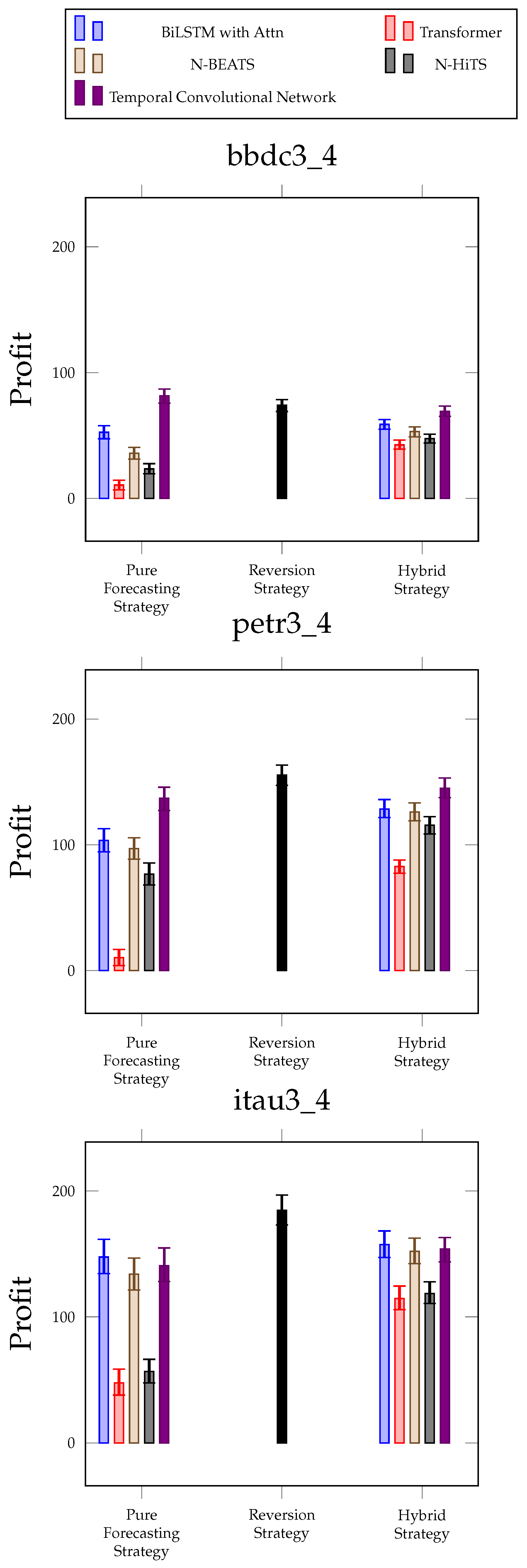
Figure 1. Profit Without Threshold: Among pure forecasting strategies, the Temporal Convolutional Network stands out as the overall best in terms of profit. However, the reversion method (shown in black) is often as good or better, with greater profits compared to the hybrid method.
Forecasting 06 00024 g001
Figure 2. Profit-per-Trade Without Threshold: The hybrid approach performs the best, especially when combining the reversion method with either the Temporal Convolutional Network or the BiLSTM with Attention.
Forecasting 06 00024 g002
Figure 3. Sharpe Ratio Without Threshold: The Sharpe Ratio is highest for the hybrid approach, especially when utilizing the Temporal Convolutional Network with the reversion method.
Forecasting 06 00024 g003
Figure 4. Profit for Static Threshold Strategy: Implementing a threshold up to 0.00025 does not diminish the profit of the reversion strategy. However, it does result in a reduction in the number of trades by 54.3%, 73.8%, and 41.6% on the bbdc3_4, petr3_4, and itau3_4 datasets, respectively. Furthermore, an increase in the threshold value beyond zero reduces the profit of both the pure and hybrid forecasting strategies, whereas an increase beyond 0.00025 decreases the profit of the reversion strategy.
Forecasting 06 00024 g004
Figure 5. Profit-per-Trade Static Threshold: The largest profit-per-trade is generated by the hybrid strategy with the largest threshold.
Forecasting 06 00024 g005
Figure 6. Dynamic thresholds are expressed as percentiles of the absolute value of the minute-by-minute change in ratio. Since the ratios observed by the base and pure forecasting strategies are different, we generate a set of dynamic thresholds for each of them. The generation of these thresholds uses only the training and validation data. The forecasting strategy is Temporal Convolutional Network. Higher percentiles lead to fewer trades and less profits.
Forecasting 06 00024 g006
Figure 7. As in the previous figure, dynamic thresholds are expressed as percentiles of the absolute value of the minute-by-minute change in ratio. The forecasting strategy is Temporal Convolutional Network. Higher percentiles lead to higher profits per trade.
Forecasting 06 00024 g007
Figure 8. Average Profit-per-Trade with Transaction Costs: The hybrid strategy performs better than mean reversion and pure forecasting using Temporal Convolutional Network. Increasing the threshold overcomes the transaction costs and leads to higher profits per trade.
Forecasting 06 00024 g008
Table 1. Chosen companies and how many milliseconds have at least one trade and how many minutes have at least one trade.
CompanyTickerTypeSectorMilliseconds Having TradesMinutes Having Trades
Petrobraspetr3ordinarygas and oil7,602,60695,606
Petrobraspetr4preferredgas and oil25,610,05295,853
Banco Itauitub3ordinaryBanks4,064,90176,450
Banco Itauitub4preferredBanks12,918,95795,885
Banco Bradescobbdc3ordinaryBanks1,555,96073,266
Banco Bradescobbdc4preferredBanks11,696,68596,120
Table 2. Comparative analysis of Forecasting Model Accuracy. N-BEATS has the lowest MAPE and sMAPE scores on the petr3_4 dataset. Temporal Convolutional Network has the lowest RMSE, MASE, MAPE, and sMPAE scores on the other datasets. This shows that the Temporal Convolutional Network predicts the numerical change in return most accurately.
DatasetPrediction
Error
Models
Bidirectional
LSTM
TransformerN-BEATSN-HiTSTemporal Convolutional
Network
bbdc3_4RMSE0.003040.002960.001310.001410.00115
MASE13.6474910.583632.096532.234071.47245
MAPE0.162950.232220.085830.094610.07035
sMAPE0.162740.232540.085790.094550.07034
petr3_4RMSE0.006920.003020.000840.001220.00097
MASE25.8679622.526202.116963.142581.75426
MAPE0.250420.249150.054150.071970.05509
sMAPE0.248590.249490.054160.071920.05507
itau3_4RMSE0.003190.002050.005050.004310.00144
MASE35.9740223.3904912.6737411.506403.06157
MAPE0.250890.207590.370370.329990.12194
sMAPE0.251570.207870.372130.331280.12206
Table 3. Confusion matrix of the trading strategies on the bbdc3_4 dataset regarding the direction of the change of ratio. When the predicted change is positive (ratio increases) and the actual direction is positive, that is a true positive (TP). When the predicted direction is positive and that is a false positive (FP). And so on. The Transformer model combined with a hybrid trading strategy has the highest F1 score.
ModelsStrategyPredicted PositivePredicted NegativeF1 Score
TPFPFNTN
Bidirectional
LSTM
Pure Forecasting Strategy73656064269641190.627
Reversion Strategy47042537244047150.654
Hybrid Strategy37791927106325610.716
TransformerPure Forecasting Strategy992798871342960.664
Reversion Strategy47042537244047150.654
Hybrid Strategy468625211032570.781
N-BEATSPure Forecasting Strategy1272508878996750.214
Reversion Strategy47042537244047150.654
Hybrid Strategy1158445241646960.447
N-HiTSPure Forecasting Strategy687271937499120.124
Reversion Strategy47042537244047150.654
Hybrid Strategy633234241947020.323
Temporal
Convolutional
Network
Pure Forecasting Strategy47472467531477160.549
Reversion Strategy47042537244047150.654
Hybrid Strategy31351341200242710.652
Table 4. Confusion matrix of the trading strategies on the petr3_4 dataset. The Transformer model combined with a hybrid trading strategy has the highest F1 score.
ModelsStrategyPredicted PositivePredicted NegativeF1 Score
TPFPFNTN
Bidirectional
LSTM
Pure Forecasting Strategy11,3098921689991820.588
Reversion Strategy10,5126784687810,4850.606
Hybrid Strategy76684598376166450.647
TransformerPure Forecasting Strategy17,38617,1478229560.659
Reversion Strategy10,5126784687810,4850.606
Hybrid Strategy10,12765424016750.744
N-BEATSPure Forecasting Strategy16,24114,186196739170.667
Reversion Strategy10,5126784687810,4850.606
Hybrid Strategy10,4546703190138210.708
N-HiTSPure Forecasting Strategy3479194814,72916,1550.294
Reversion Strategy10,5126784687810,4850.606
Hybrid Strategy32851752672610,3190.436
Temporal
Convolutional
Network
Pure Forecasting Strategy10,2307092797811,0110.575
Reversion Strategy10,5126784687810,4850.606
Hybrid Strategy80484775513785420.618
Table 5. Confusion matrix of the trading strategies on the itau3_4 dataset. The Transformer model combined with a hybrid trading strategy has the highest F1 score.
ModelsStrategyPredicted PositivePredicted NegativeF1 Score
TPFPFNTN
Bidirectional
LSTM
Pure Forecasting Strategy13,07610,122317859460.662
Reversion Strategy87184975510086660.633
Hybrid Strategy78553953172739860.734
TransformerPure Forecasting Strategy15,93015,3823246860.669
Reversion Strategy87184975510086660.633
Hybrid Strategy865749092415820.770
N-BEATSPure Forecasting Strategy11,9739255428168130.638
Reversion Strategy87184975510086660.633
Hybrid Strategy75533755222244310.716
N-HiTSPure Forecasting Strategy15,77514,85247912160.672
Reversion Strategy87184975510086660.633
Hybrid Strategy8674491439410820.765
Temporal
Convolutional
Network
Pure Forecasting Strategy13,19510,308305957600.663
Reversion Strategy87184975510086660.633
Hybrid Strategy79524033173939120.733
Table 6. Effect of transaction costs on the total profit of each strategy. The profits are of course lower. However, with the highest dynamic threshold, our approach is still capable of delivering profits. While the table shows that the total profits are consistently best using the reversion strategy here, this would change if the brokerage fees were slightly higher, because then the strategy with the highest profit per trade would also yield the highest profit.
Pair of StocksStrategyProfit before FeesProfit after Fees
bbdc3_4Pure Forecasting Strategy7.82914.9139
Reversion Strategy37.663216.0140
Hybrid Strategy11.76617.2873
petr3_4Pure Forecasting Strategy64.96759.4263
Reversion Strategy87.010314.2168
Hybrid Strategy38.414412.9912
itau3_4Pure Forecasting Strategy29.609717.0472
Reversion Strategy86.744036.9860
Hybrid Strategy32.187324.7291
Disclaimer/Publisher’s Note: The statements, opinions and data contained in all publications are solely those of the individual author(s) and contributor(s) and not of MDPI and/or the editor(s). MDPI and/or the editor(s) disclaim responsibility for any injury to people or property resulting from any ideas, methods, instructions or products referred to in the content.