Abstract
Deep learning has recently demonstrated the ability to predict long-term patient risk and its stratification when trained on imaging data such as chest radiographs. However, existing methods formulate estimating patient risk as a binary classification, typically ignoring or limiting the use of temporal information, and not accounting for the loss of patient follow-up, which reduces the fidelity of estimation and limits the prediction to a certain time horizon. In this paper, we demonstrate that deep survival and time-to-event prediction models can outperform binary classifiers at predicting mortality and risk of adverse health events. In our study, deep survival models were trained to predict risk scores from chest radiographs and patient demographic information in the Prostate, Lung, Colorectal, and Ovarian (PLCO) cancer screening trial (25,433 patient data points used in this paper) for 2-, 5-, and 10-year time horizons. Binary classification models that predict mortality at these time horizons were built as baselines. Compared to the considered alternative, deep survival models improve the Brier score (5-year: 0.0455 [95% CI, 0.0427–0.0482] vs. 0.0555 [95% CI, (0.0535–0.0575)], p < 0.05) and expected calibration error (ECE) (5-year: 0.0110 [95% CI, 0.0080–0.0141] vs. 0.0747 [95% CI, 0.0718–0.0776], p < 0.05) for those fixed time horizons and are able to generate predictions for any time horizon, without the need to retrain the models. Our study suggests that deep survival analysis tools can outperform binary classification in terms of both discriminative performance and calibration, offering a potentially plausible solution for forecasting risk in clinical practice.
1. Introduction
Chest radiography is a common diagnostic tool for lung disorders and offers prognostic value in terms of overall patient health and well-being. The ability to prognosticate patient susceptibility to an adverse outcome such as death or serious complications using such inexpensive medical testing is therefore of immense interest. Indeed, recent advances in deep learning [1] have demonstrated that, e.g., convolutional neural network (CNN) approaches perform well in diagnosing conditions from chest radiograms, in some cases even outperforming trained radiologists [2,3,4,5,6,7].
The ability to consolidate the likelihood of adverse outcomes into a single scalar risk estimate is an exciting prospect as such a score could be utilized to stratify patients based on their risk levels and to prioritize subsequent treatment and interventions, helping improve overall longevity. However, deep learning models are typically trained to predict multiple adverse diagnoses [8], and consolidating those individual diagnoses into a singular risk score or estimate can be a challenging task.
In studies that involve risk estimation from medical imaging data [9,10,11,12,13,14], the time-to-event outcome is binarized as an indicator of whether a patient survived beyond a certain point in time (such as a 5-year risk), and imaging data from individuals who were lost to follow-up (censored) are discarded when training the model. However, long-term patient risk levels might vary over time depending on patient physiology, medical history, and demographics. This can happen as a result of time-varying covariates, where some measurements or observations change over time. For example, in studying cancer risk, smoking status can be a time-varying covariate [15]. As a result, modeling patients’ risk at a fixed time in the future might be insufficient to obtain an overall sense of their prognosed health and well-being. Furthermore, in real-world observational studies, patients cannot be followed up indefinitely due to resource constraints and study design. A large number of patients thus might be lost to follow-up before an event of interest is observed in them. Moreover, a binary classifier is only able to make predictions at the fixed time horizon that is chosen to be the threshold for the binary targets, which makes it less flexible in that if a user wants the patient risk at a different time, the model needs to be trained again on the new binary target.
Deep survival analysis and time-to-event prediction aim to address those limitations by modeling time as a continuous random variable and incorporating censoring in the estimation of patient risk. Survival analysis is a class of statistical methods for estimating the time until an event occurs. As opposed to binary classification, the time-to-event outcome for a particular individual is considered to be a continuous random variable. In this study, we were interested in estimating the risk of a patient experiencing mortality within a time horizon, given a chest radiograph and a set of demographic covariates. We assumed that an observation can be right-censored, which means that the observation of a subject can be terminated before death occurs.
Cox proportional hazards (CPH) [16] is arguably one of the most popular approaches for analyzing time-to-event survival data. The CPH model makes a proportional hazards assumption, stating that the ratio between the hazard rates of two individuals is constant over all time horizons (please refer to Appendix B for a more detailed description). In real-world application scenarios, however, the proportional hazards assumption may be overly restrictive or not hold at all. The Deep Survival Machines (DSM) [17] approach does not assume proportional hazards. Appendix C explains the mechanism of DSM.
In this paper, we examine a multimodal application of time-to-event data to predict long-term patient risk from chest radiographs and patient demographic data. In particular, we use models such as CPH and DSM as replacements for binary models. We aim to demonstrate that the proposed approach is able to generate predictions at any time horizon while achieving superior discriminative performance and calibration. The source code is available at https://github.com/autonlab/Deep_Chest_Survival (accessed on 21 May 2024).
2. Materials and Methods
The dataset used in this study is from the randomized controlled Prostate, Lung, Colorectal, and Ovarian (PLCO) cancer screening trial [18]. The goal of the trial was to investigate whether screening has an effect on cancer-related mortality.
At 10 screening centers nationwide, 154,934 participants were enrolled between November 1993 and September 2001. One coordinating center performed data management and trial coordination. Each arm involved 37,000 females and 37,000 males aged 55–74 at entry. In the control arm, participants received their usual medical care. In the intervention arm, women received chest X-rays, flexible sigmoidoscopy, CA125, and transvaginal ultrasound (TVU), and men received chest X-rays, flexible sigmoidoscopy, serum prostate-specific antigen (PSA), and digital rectal exams (DREs). PSA and CA125 were performed at entry, then annually for 5 years. DRE, TVU, and chest X-ray exams were performed at entry, then annually for 3 years. Only two annual repeat X-ray exams were performed for non-smokers. Sigmoidoscopy was performed at entry, then at the 5-year point.
A radiologist interpreted each posteroanterior chest X-ray and radiologists’ impressions were included in the dataset. Participants were followed for at least 13 years. Deaths during the trial were confirmed by mailed annual study update (ASU) and linkage to the National Death Index (NDI). Causes of death during the trial were also determined.
Data were collected on forms designed for an NCS OpScan 5 optical-mark reader, and then automatically loaded into a database. Information collected at screening centers went through a hub through modems using common carrier lines. Additional details about the PLCO dataset can be found in [19,20,21].
The dataset includes radiologists’ impressions that indicate whether abnormalities exist. The survival curves based on the time-to-death data of each patient are shown in Figure 1. For demonstration, we selected the noted presence of bone/soft tissue lesions, cardiac abnormalities, COPD, granuloma, pleural fibrosis, pleural fluid, scarring, radiographic abnormalities, mass, pleural, nodule, atelect, hilar, infiltrate, and other abnormalities. The curves are stratified by whether the mentioned abnormalities and lung cancer were present at the beginning of the study.
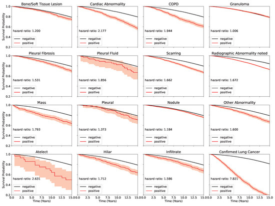
Figure 1.
Survival curves plotted with Kaplan–Meier survival estimates for phenogroups, stratified by abnormalities.
2.1. Preprocessing
In this study, we used grayscale chest radiographs, demographic data, time-to-death, and censor indicators. Demographic data record sex, race, ethnicity, cigarette smoking status, and age. Age was defined to be the age at the time of screening. Time-to-event was defined as the number of days from the chest X-ray screen to the day of death or the last known day of life (censoring time). Censor indicators were binary variables, where 0 indicated that the outcome was censored, and 1 indicated that death was observed.
In total, 89,643 images were used; 60% were used for training the model, 20% were held out as the validation data for optimizing model hyperparameters, and 20% were held out for testing and final model evaluation. We ensured that images from the same patient did not appear in more than one of the training, testing, or validation subsets of data.
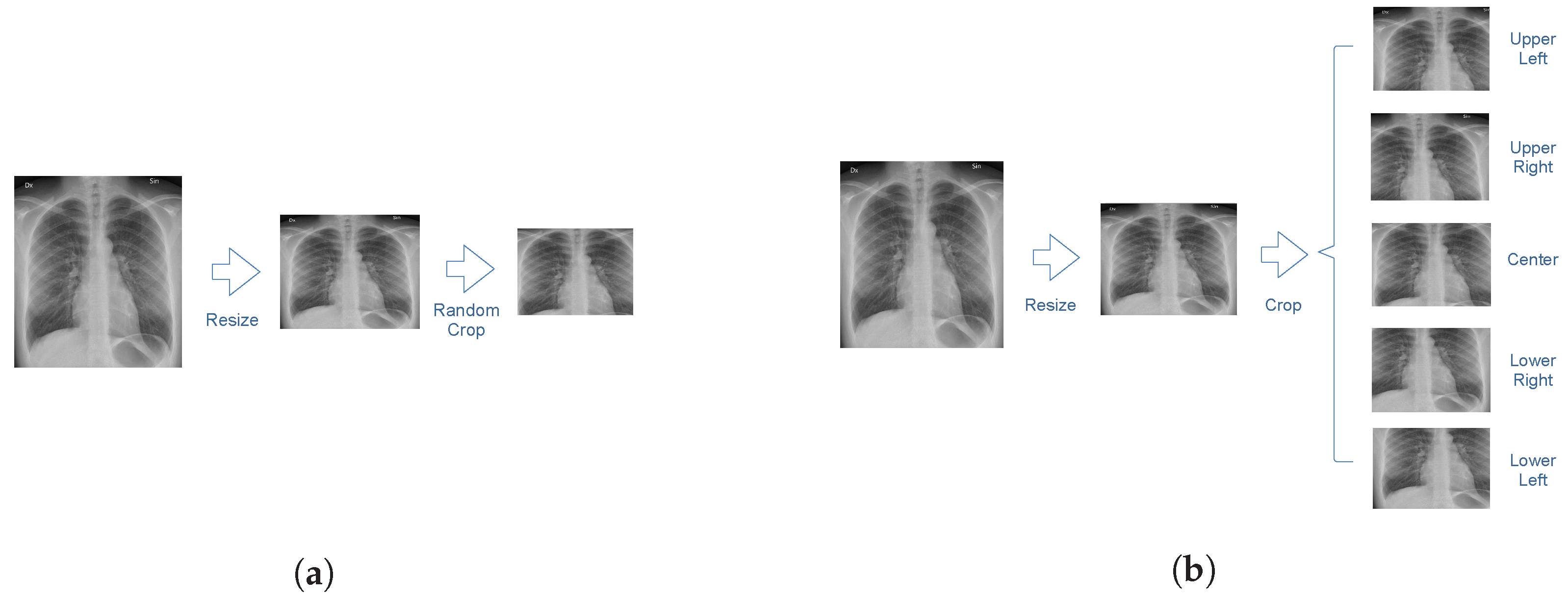
An illustration of the image preprocessing procedure is shown in Figure 2. The size of each image is 2500 by 2100 pixels. In order to reduce computational costs, each chest radiograph was resized to a 256 by 256-pixel image. Images in the training dataset were cropped to 224 by 224 pixels at a random position. Images in the testing dataset were cropped at the four corners and the center. Predictions were obtained for each crop independently and averaged to obtain a final prediction for the entire image.
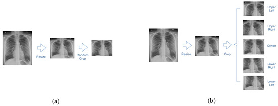
Figure 2.
An illustration of the resizing and cropping procedure. (a) Images in the training dataset were resized and cropped at a random position. (b) Images in the test dataset were resized and cropped at the corners and the center.
Statistics of data from the subset of the PLCO database used in this study are summarized in Table 1. Samples with negative times were discarded.

Table 1.
Statistics of the subset of PLCO data used in this study.
2.2. Evaluation Metrics
We evaluated the performance of the considered models using the Brier score [22], the concordance index based on the inverse probability of censoring weights [23], the cumulative/dynamic area under the receiver operating characteristic curve (AUC) [24,25], and the expected calibration error (ECE) [26] for 2-year, 5-year, and 10-year time horizons. Additional details on evaluation metrics can be found in Appendix D. Bootstrapping with 100 samples was performed to obtain 95% confidence intervals. Samples were drawn from test-set predictions with 100 replacements.
The Brier score measures the average squared distance between the actual survival probability and the predicted survival probability for a given time horizon. The higher the Brier score, the worse the discriminative performance of the model.
The concordance index measures discriminative performance in terms of the probability of assigning higher risk to subjects with shorter times-to-events by calculating the ratio of the number of correctly ordered pairs of patients, based on their actual outcomes, to the total number of such pairs. The concordance index, based on the inverse probability of censoring weights, uses the Kaplan–Meier estimator to estimate the censoring distribution.
The receiver operating characteristic (ROC) curve is typically depicted with the true positive rate as a function of the false positive rate for varying sensitivity thresholds of a binary discrimination or detection model. The higher the AUC, the more accurately ranked the test data instances, i.e., the model gives the positive samples higher scores than the negatives.
The expected calibration error (ECE) is calculated by splitting data sorted by predicted probabilities into subsequent bins and averaging the per-bin differences between predicted probabilities and true probabilities. The lower the ECE, the better the model prediction scores correlate with true probabilities; hence there is less miscalibration.
2.3. Methods
In this work, we propose a novel model that extracts survival probabilities from chest X-rays, trained in an end-to-end fashion. Our model consists of an encoder and a survival model that are connected by a multilayer perceptron, as shown in Figure 3. The encoder is based on a DenseNet model [27] that takes the chest X-rays as inputs and outputs a numeric vector as the representation of the images. The encoder was adopted from the TorchXRayVision Python package [28] and pre-trained on other chest X-ray datasets, including CheXpert and MIMIC-CXR.

Figure 3.
Model architecture. The proposed model takes chest radiographs and demographic information as inputs and outputs survival probabilities. The encoder (DenseNet-121) extracts information from the images, which is then combined with demographic information as inputs to the survival model.
The survival models are adopted from the auton-survival Python package [29]. A deep neural network version of Cox proportional hazards (DCPH) and DSM are used alternatively. They take the vector representation of chest X-rays and demographic data as inputs and output risk scores for certain time horizons. In this study, we predicted 2-year, 5-year, and 10-year mortality.
We compared the proposed models with a common approach from the literature, such as CXR-risk in Lu et al. [9], which is to train a model to predict mortality for a fixed time horizon. We denote such a model as Thresholded Binary Classification (TBC). In TBC, the time-to-event outcome is binarized to a label representing survival beyond t years from the time the X-ray was obtained, . Specifically, cases where censoring or survival times are longer than t are classified as “survived”, and non-censored cases where the times are shorter than or equal to t are classified as “dead”. The rest, where the times are shorter than t and censored, are ignored. The number of samples in each category is summarized in Table 2.

Table 2.
The number of samples in each category.
A hyperparameter search was performed by finding model configurations that minimized the mean Brier score for 2-, 5-, and 10-year time horizons in the validation dataset. Additional implementation details are presented in Appendix E.
3. Results
The number of patients at risk before different times, defined as those who have censoring or survival times greater than the corresponding time, is shown in Table 3.

Table 3.
Number of patients at risk before 0, 2, 5, 10, 15, and 20 years.
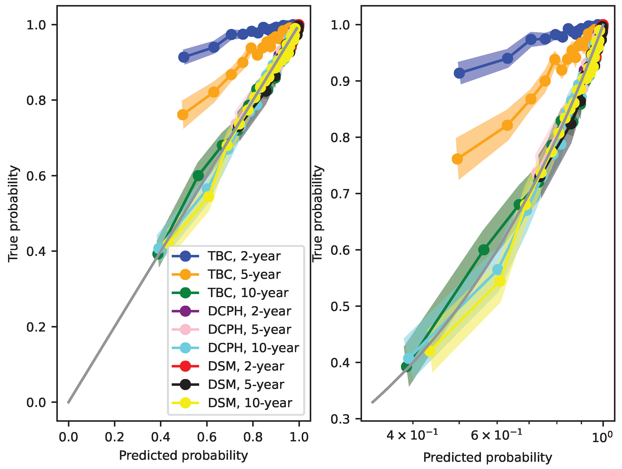
The performance of each model measured with the Brier score, concordance index, AUC, and ECE for 2-year, 5-year, and 10-year time horizons is summarized in Table 4. Two-sample t-tests were performed to compare the performance of TBC and DSM, and the performance of TBC and DCPH. Calibration curves plotted with linear and logarithmic scales are shown in Figure 4.

Table 4.
Brier score, concordance index, AUC, and ECE evaluated on test dataset with bootstrapping. Best performances are in bold. The 95% confidence intervals are shown in parentheses. TBC (baseline model) performed the worst. p-values for the two-sample t-tests between TBC and DSM and between TBC and DCPH are shown under confidence intervals. p-values lower than 0.05 are in bold.
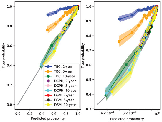
Figure 4.
Calibration plots for TBC, DCPH, and DSM at 2-year, 5-year, and 10-year time horizons, with 95% confidence intervals (left: linear scale, right: logarithmic scale). TBC calibration at 2-year and 5-year time horizons is significantly worse than the proposed alternatives.
DSM and DCPH perform no worse than TBC with respect to the Brier score, concordance index, AUC, and ECE. In particular, they perform significantly better on shorter-horizon (2-year and 5-year) Brier scores and calibration. The 2-year and 5-year Brier scores of TBC are 0.0354 and 0.0555, whereas those of DSM are 0.0132 and 0.0455 and those of DCPH are 0.0132 and 0.0456. The 2-year, 5-year, and 10-year ECEs of TBC are 0.1126, 0.0747, and 0.0216, whereas those of DSM are 0.0052, 0.0110, and 0.0152 and those of DCPH are 0.0043, 0.0089, 0.0135. The calibration curves for 2-year and 5-year TBC also significantly deviate from the perfectly calibrated line, compared to other curves. These results suggest that the proposed models offer improved discriminative performance and calibration when compared to a commonly used binary model.
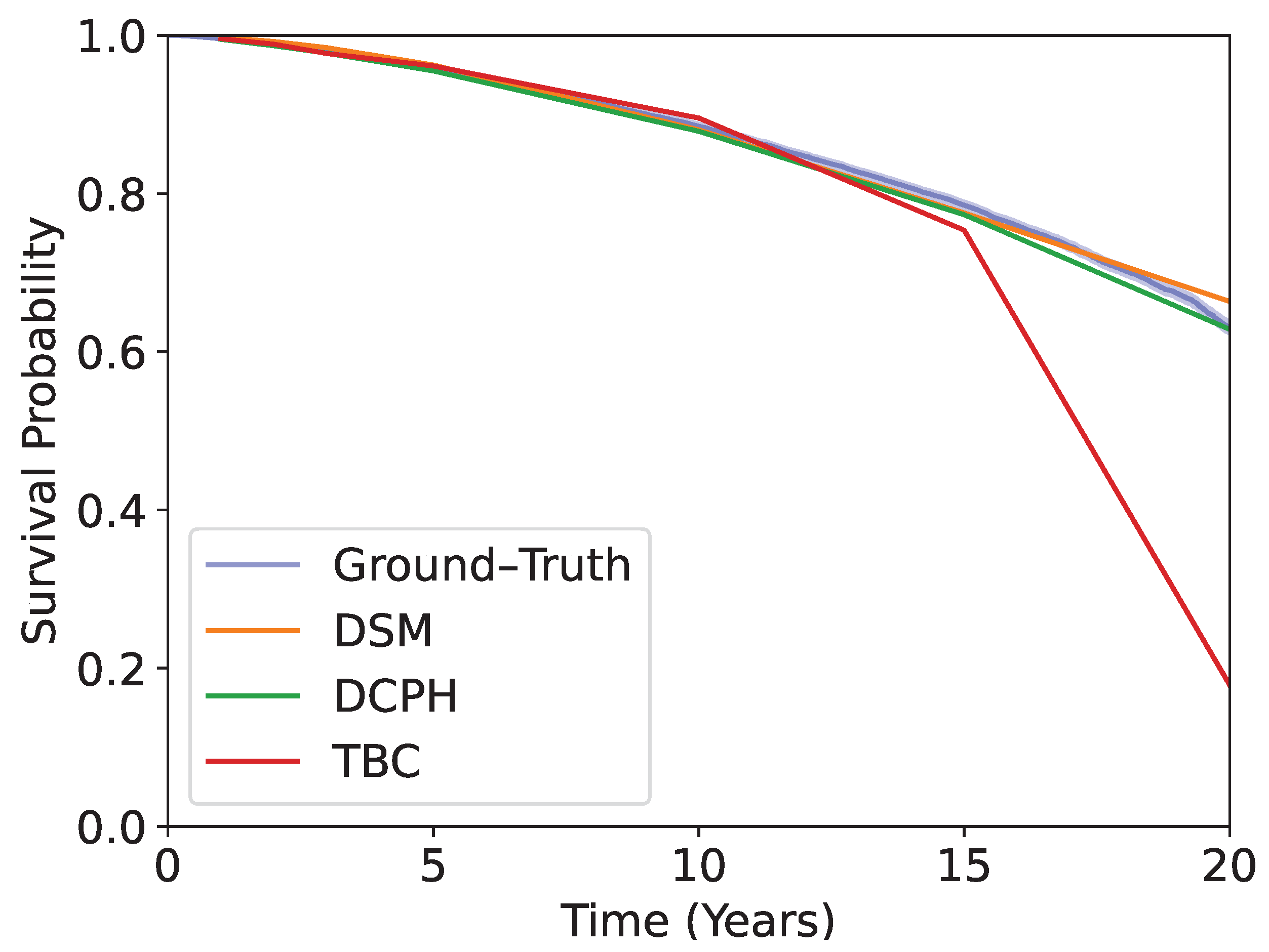
Kaplan–Meier curves obtained using the test dataset are shown in Figure 5. The blue curve is obtained by using the ground-truth time-to-event. The rest shows the predicted survival probabilities averaged over the test dataset, using DSM, DCPH, and TBC. The models are evaluated at 1-, 2-, 3-, 5-, 10-, 15-, and 20-year time horizons. DSM and DCPH provide curves that match the ground-truth Kaplan–Meier curve more closely than TBC, especially at longer time horizons.
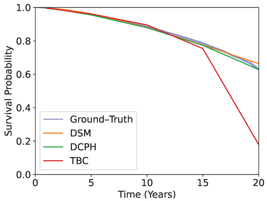
Figure 5.
The Kaplan–Meier curve obtained from each patient in the test dataset, plotted with the ground–truth time-to-event, and average predicted survival probabilities at each time horizon using TBC, DSM, and DCPH. DSM and DCPH provide more accurate estimations.
DSM does not show significantly improved performance when compared to DCPH. This suggests that, with regard to the dataset we used, the assumption of proportional hazards does not substantially impact predictive power and suggests that there is no substantial prognostic value in non-proportional hazards.
4. Discussion
We demonstrated that deep learning survival models that use time-to-event and censor indicators can offer more flexibility and perform better at predicting long-term mortality than commonly used binary classifiers, in terms of Brier score and ECE, on multiple time horizons.
Patient risk prediction from imaging data using deep learning is traditionally performed with a binary mortality outcome variable, not accounting for censored outcomes. Lu et al. [9] demonstrated that CNNs have the prognostic capability to assess a patient’s risk of morality over long time horizons (12 years) in a large cohort of patients from the Prostate, Lung, Colorectal, and Ovarian (PLCO) cancer screening trial [18]. They further validated their estimated risk score on an internal held-out set as well as on an external study, the National Lung Screening Trial (NLST). Other studies applied similar techniques to multiple contexts and various time horizons [10,11,12,13,14]. For instance, Kolossváry et al. [11] used deep learning to predict 30-day all-cause mortality using chest radiographs. Raghu et al. [14] estimated postoperative mortality (30-day mortality and in-hospital mortality) after cardiac surgeries using preoperative chest X-rays.
As shown in the TBC study, a model needs to be trained on each of the time horizons of interest. It appears that these models do not necessarily reach the attainable performance, possibly due to not considering censoring information and the time-varying effects of covariates. Survival analysis (DSM and DCPH) can incorporate these factors natively.
CPH is a semiparametric method that requires no predefined probability function to represent survival times, but assumes proportional hazards. It estimates the hazard, which is defined as the instantaneous probability that an event will occur. DeepSurv [30] is a deep learning framework based on CPH. The hazard function in DeepSurv is determined by the parameters of a trained deep neural network.
DSM adds flexibility by modeling the survival distribution as a mixture of multiple component distributions. It assumes that each component distribution is parametric, and does not assume proportional hazards. The parameters of each component and mixture weights are learned from data using neural networks. The individual survival distribution is estimated as an average of the learned distributions weighted by the learned mixture weights.
We expected that DSM would perform better than DCPH, since it imposes fewer assumptions. However, in the specific case of the PLCO dataset, relaxing the assumption of proportional hazards does not appear to yield additional benefits, since the performances of DSM and DCPH are comparable.
Our study has limitations. For instance, as shown in Table 1, 50% of patients are between 58 and 73 years of age, and only 12.68% are non-White. Therefore, those who are younger and non-White may not be adequately represented in the training data, resulting in a bias toward those who are older and White, and potentially impacting the models’ effectiveness in promoting patient care uniformly across subpopulations. Further studies are needed to assess the performance of the proposed models when used on populations of different ages and races than those represented in the data used in the current study.
One of our future steps involves the application of the proposed models to counterfactual phenotyping, where groups of individuals belong to underlying clusters and demonstrate heterogeneous treatment effects [31]. This may provide insights into measuring the distinctive effects of interventions on certain subgroups of patients and enable personalized interventions that lead to optimal outcomes.
Author Contributions
Conceptualization, C.N., M.L. and A.D.; methodology, C.N. and M.L.; software, M.L. and C.N.; validation, M.L. and C.N.; formal analysis, M.L. and C.N.; investigation, M.L. and C.N.; resources, C.N. and A.D.; data curation, C.N.; writing—original draft preparation, M.L.; writing—review and editing, M.L., C.N. and A.D.; visualization, M.L.; supervision, A.D.; project administration, C.N. and A.D.; funding acquisition, A.D. All authors have read and agreed to the published version of the manuscript.
Funding
This work was partially funded by the Defense Advanced Research Projects Agency under award FA8750-17-2-0130 and by a Space Technology Research Institutes grant from NASA’s Space Technology Research Grants Program.
Data Availability Statement
The original data presented in the study are openly available at https://cdas.cancer.gov/plco/ (accessed on 21 May 2024).
Conflicts of Interest
The authors declare no conflicts of interest.
Abbreviations
The following abbreviations are used in this manuscript:
| PLCO | Prostate, Lung, Colorectal, and Ovarian |
| ECE | expected calibration error |
| CNN | convolutional neural network |
| NLST | National Lung Screening Trial |
| CPH | Cox proportional hazards |
| DSM | Deep Survival Machines |
| ASU | annual study update |
| NDI | National Death Index |
| AUC | area under the receiver operating characteristic curve |
| ROC | receiver operating characteristic |
| DCPH | deep Cox proportional hazards |
| TBC | Thresholded Binary Classification |
| BS | Brier Score |
| TPR | true positive rate |
| TNR | true negative rate |
Appendix A. Censoring and Time-to-Event Predictions
We are interested in estimating , the risk of a patient experiencing mortality within a time horizon , given a chest radiograph and a set of demographic covariates . We assume that observations on T can be right-censored, which means that the observation is terminated before death occurs.
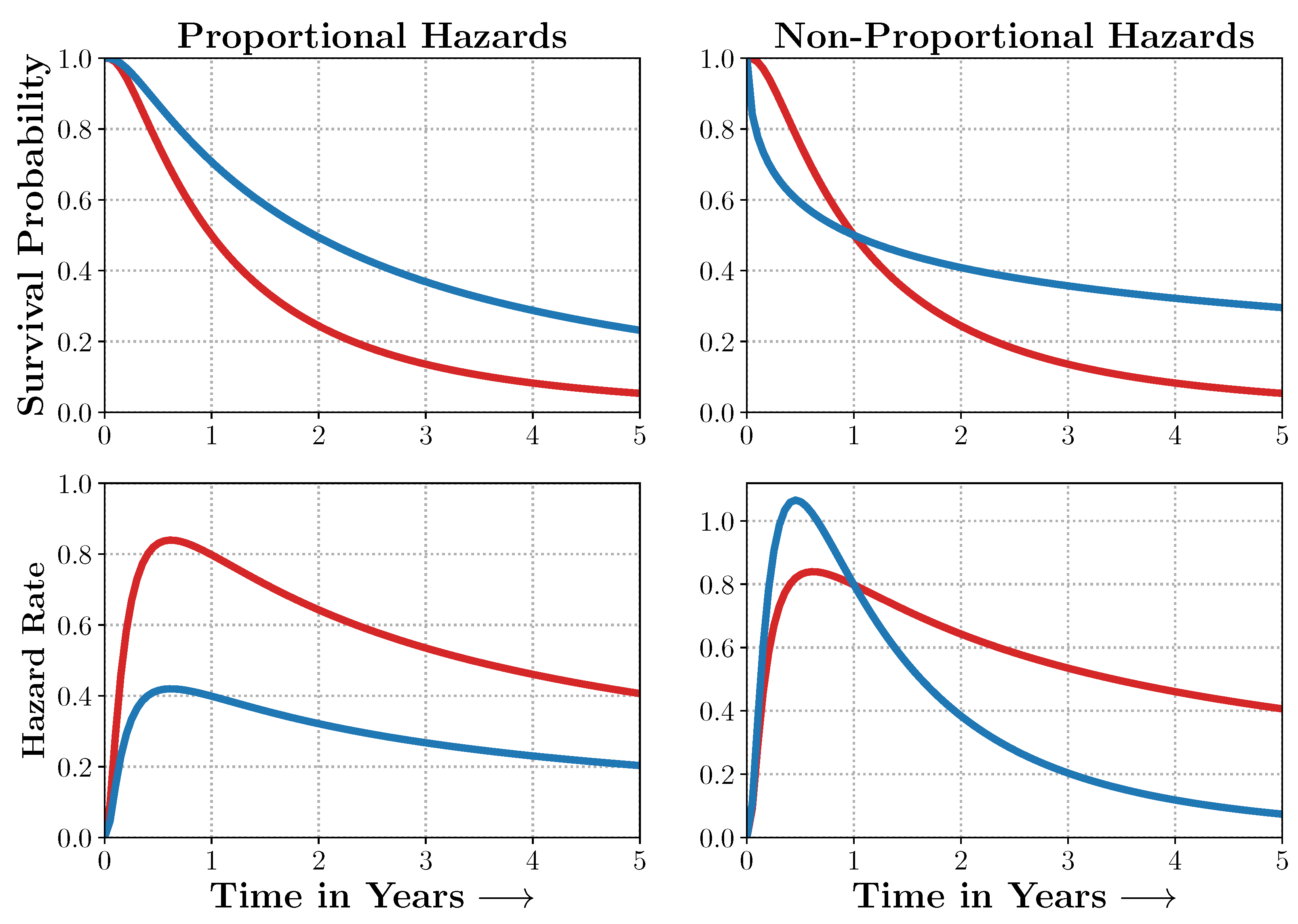
Censoring makes it challenging to learn an estimator of survival. As evidenced in Figure A1, the censored patients need to be accounted for to obtain an unbiased estimate of patient survival. Standard survival models such as the Cox model make strong assumptions about the distribution of the event times. Hence, they cannot generalize to situations where the assumptions are violated (Figure A2).
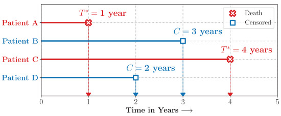
Figure A1.
Censoring and Time-to-Event Predictions. Patients A and C died 1 and 4 years from entry into the study, whereas Patients B and D exited the study without experiencing death (were lost to follow-up) at 2 and 3 years from entry into the study. Time-to-event and survival regression thus involve estimates that are adjusted for individuals whose outcomes were censored. Source: Adapted from [29].
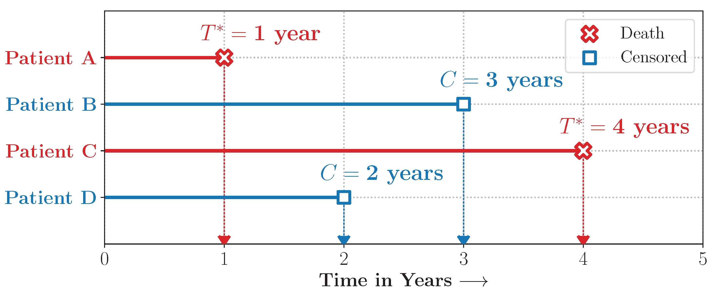

Figure A2.
Non-Proportional Hazards. When the proportional hazards assumptions are satisfied, the survival curves and their corresponding hazard rates dominate each other and do not intersect. In many real-world scenarios, however, the survival curves do. Models such as Deep Survival Machines include flexible estimators of times-to-events in the presence of non-proportional hazards. Source: Adapted from [29].
Appendix B. Additional Details on Proportional Hazards Model
Cox proportional hazards (CPH) makes the proportional hazards assumption that the ratio between two hazards is constant over time [16]. The hazard as a function of some time t is defined as the probability that given that a patient survives t, the patient will not survive , and approaches 0 (Equation (A1)).
CPH models the hazard as Equation (A2), given covariates , where p is the number of predictors, and n is the number of patients. The parameters of the model are . is known as the baseline hazard function.
The proportional hazards assumption comes from the fact that the proportion of two hazard functions is fixed, since .
We estimated that are the ones that maximize the partial likelihood(Equation (A3)), where are patients whose outcomes are not censored, and is the set of patients who have not experienced the event at time .
DeepSurv [30] is a deep neural network implementation of CPH. It estimates the risk function of an individual with covariates x, parametrized by the weights of a multi-layer perceptron. The loss function is the negative log partial likelihood (Equation (A4)).
Appendix C. Additional Details on Deep Survival Machines
In this section, we describe Deep Survival Machines, which models the time-to-event distribution. The DSM model involves modeling the time-to-event distribution as a fixed-size mixture of K parametric survival distributions. This allows the model to generalize to situations where the survival curves intersect (a clear violation of the proportional hazards assumption.). The final time-to-event outcome is determined by averaging over the latent . We provide DSM in plate notation in Figure A3.
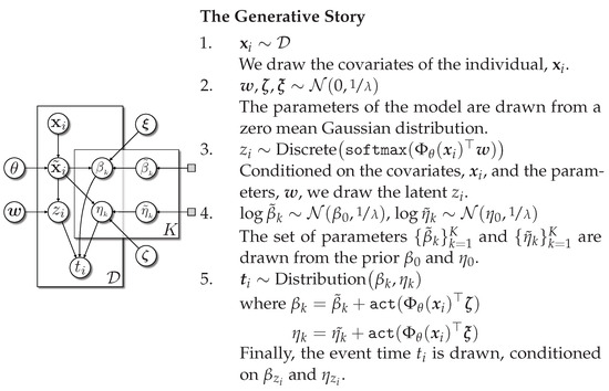
Figure A3.
Deep Survival Machines in plate notation. Source: Adapted from [17].
Figure A3.
Deep Survival Machines in plate notation. Source: Adapted from [17].

Appendix D. Censoring Adjusted Evaluation Metrics
- Brier Score (BS): The Brier score involves computing the mean squared error of the estimated survival probabilities, , at a specified time horizon, t. As a proper scoring rule, the Brier score gives a sense of both discrimination and calibration.
Under the assumption that the censoring distribution is independent of the time-to-event, we can obtain an unbiased, censoring adjusted estimate of the Brier score using the inverse probability of censoring weights (IPCW) from a Kaplan–Meier estimator of the censoring distribution, , as proposed in [32,33].
Area under ROC Curve (AUC): ROC curves are extensively used in classification tasks where the true positive rate (TPR) is plotted against the false positive rate (1-true negative rate, or TNR) to measure the model’s discriminative power over all output thresholds.
To enable the use of ROC curves to assess the performance of survival models subject to censoring, we employed the technique proposed by [24,25], which treats the TPR as time-dependent on a specified horizon, t, and adjusts survival probabilities, , using the IPCW from a Kaplan–Meier estimator of the censoring distribution, . Estimating the TNR requires observing outcomes for each individual; only uncensored instances are used. Refer to [34] for details on computing ROC curves in the presence of censoring.
Time-Dependent Concordance Index ( ): The concordance index compares risks across all pairs of individuals within a fixed time horizon, t, to estimate the ability to appropriately rank instances relative to each other in terms of their risks, .
We employed the censoring adjusted estimator for , which exploits IPCW estimates from a Kaplan–Meier estimate of the censoring distribution. Further details can be found in [23,35].
Expected Calibration Error (ECE): The ECE measures the average absolute difference between the observed and expected (according to the risk score) event rates, conditional on the estimated risk score. At time t, let the predicted risk score be . Then, the ECE approximates
by partitioning the risk scores R into q quantiles and computing the Kaplan–Meier estimate of the event rate. , and the average risk score, , in each bin. Altogether, the estimated ECE is
In practice, we fixed the number of quantiles to 20 for our experiments.
Appendix E. Implementation Details
All experiments were run on NVIDIA RTX A6000, with Python 3.9.12 and Pytorch 1.11.0. Statistical analysis was performed with Python 3.9.12.
We performed a hyperparameter search by searching for the hyperparameters that yielded the lowest validation Brier score.
For DCPH, DSM, and TBC models, layer sizes (the number of neurons in each hidden layer of survival models) are searched from [( ) (no hidden layers), (64) (one hidden layer with 64 neurons), (64, 64) (two hidden layers with 64 neurons each), (128) (one hidden layer with 128 neurons), and (128, 128) (two hidden layers with 128 neurons each)]. For DSM models, in addition to layer sizes, the number of underlying distributions k is searched from [2, 3, 4, 6], temperatures from [1, 100, 500, 1000], and elbo from [True, False]. The configurations with the best validation performance are presented in Table A1.
Adam optimizer with a learning rate of was used for all models. The distribution for all DSM models was Weibull distribution. The training batch size was 64, and the validation batch size was 32. Models were trained for 10 epochs, with a patience of 3.

Table A1.
Hyperparameter configurations that yielded the best validation performance.
Table A1.
Hyperparameter configurations that yielded the best validation performance.
| DSM | DCPH | TBC, 2-Year | TBC, 5-Year | TBC, 10-Year | |||
|---|---|---|---|---|---|---|---|
| Layer Size | k | Temperature | Elbo | Layer Size | Layer Size | ||
| (128) | 4 | 1 | True | (64, 64) | (64) | (64, 64) | (128) |
References
- Goodfellow, I.; Bengio, Y.; Courville, A. Deep Learning; MIT Press: Cambridge, MA, USA, 2016. [Google Scholar]
- Baltruschat, I.M.; Nickisch, H.; Grass, M.; Knopp, T.; Saalbach, A. Comparison of Deep Learning Approaches for Multi-Label Chest X-ray Classification. Sci. Rep. 2019, 9, 6381. [Google Scholar] [CrossRef] [PubMed]
- Rajpurkar, P.; O’Connell, C.; Schechter, A.; Asnani, N.; Li, J.; Kiani, A.; Ball, R.L.; Mendelson, M.; Maartens, G.; van Hoving, D.J.; et al. CheXaid: Deep Learning Assistance for Physician Diagnosis of Tuberculosis Using Chest x-Rays in Patients with HIV. NPJ Digit. Med. 2020, 3, 115. [Google Scholar] [CrossRef] [PubMed]
- Rajpurkar, P.; Irvin, J.; Zhu, K.; Yang, B.; Mehta, H.; Duan, T.; Ding, D.; Bagul, A.; Langlotz, C.; Shpanskaya, K.; et al. CheXNet: Radiologist-Level Pneumonia Detection on Chest X-rays with Deep Learning. arXiv 2017, arXiv:1711.05225. [Google Scholar] [CrossRef]
- Rajpurkar, P.; Irvin, J.; Ball, R.L.; Zhu, K.; Yang, B.; Mehta, H.; Duan, T.; Ding, D.; Bagul, A.; Langlotz, C.P.; et al. Deep Learning for Chest Radiograph Diagnosis: A Retrospective Comparison of the CheXNeXt Algorithm to Practicing Radiologists. PloS Med. 2018, 15, e1002686. [Google Scholar] [CrossRef] [PubMed]
- Yao, L.; Poblenz, E.; Dagunts, D.; Covington, B.; Bernard, D.; Lyman, K. Learning to Diagnose from Scratch by Exploiting Dependencies among Labels. arXiv 2018, arXiv:1710.10501. [Google Scholar] [CrossRef]
- Zhang, J.; Xie, Y.; Li, Y.; Shen, C.; Xia, Y. COVID-19 Screening on Chest X-ray Images Using Deep Learning Based Anomaly Detection. arXiv 2020, arXiv:2003.12338. [Google Scholar]
- Bakator, M.; Radosav, D. Deep Learning and Medical Diagnosis: A Review of Literature. Multimodal Technol. Interact. 2018, 2, 47. [Google Scholar] [CrossRef]
- Lu, M.T.; Ivanov, A.; Mayrhofer, T.; Hosny, A.; Aerts, H.J.W.L.; Hoffmann, U. Deep Learning to Assess Long-term Mortality From Chest Radiographs. JAMA Netw. Open 2019, 2, e197416. [Google Scholar] [CrossRef]
- Cheng, J.; Sollee, J.; Hsieh, C.; Yue, H.; Vandal, N.; Shanahan, J.; Choi, J.W.; Tran, T.M.L.; Halsey, K.; Iheanacho, F.; et al. COVID-19 Mortality Prediction in the Intensive Care Unit with Deep Learning Based on Longitudinal Chest X-rays and Clinical Data. Eur. Radiol. 2022, 32, 4446–4456. [Google Scholar] [CrossRef]
- Kolossváry, M.; Raghu, V.K.; Nagurney, J.T.; Hoffmann, U.; Lu, M.T. Deep Learning Analysis of Chest Radiographs to Triage Patients with Acute Chest Pain Syndrome. Radiology 2023, 306, e221926. [Google Scholar] [CrossRef]
- Mayampurath, A.; Sanchez-Pinto, L.N.; Carey, K.A.; Venable, L.R.; Churpek, M. Combining Patient Visual Timelines with Deep Learning to Predict Mortality. PLoS ONE 2019, 14, e0220640. [Google Scholar] [CrossRef] [PubMed]
- Panesar, S.S.; D’Souza, R.N.; Yeh, F.C.; Fernandez-Miranda, J.C. Machine Learning Versus Logistic Regression Methods for 2-Year Mortality Prognostication in a Small, Heterogeneous Glioma Database. World Neurosurg. X 2019, 2, 100012. [Google Scholar] [CrossRef] [PubMed]
- Raghu, V.K.; Moonsamy, P.; Sundt, T.M.; Ong, C.S.; Singh, S.; Cheng, A.; Hou, M.; Denning, L.; Gleason, T.G.; Aguirre, A.D.; et al. Deep Learning to Predict Mortality After Cardiothoracic Surgery Using Preoperative Chest Radiographs. Ann. Thorac. Surg. 2023, 115, 257–264. [Google Scholar] [CrossRef] [PubMed]
- Zhang, Z.; Reinikainen, J.; Adeleke, K.A.; Pieterse, M.E.; Groothuis-Oudshoorn, C.G.M. Time-Varying Covariates and Coefficients in Cox Regression Models. Ann. Transl. Med. 2018, 6, 121. [Google Scholar] [CrossRef] [PubMed]
- Cox, D.R. Regression Models and Life-Tables. J. R. Stat. Soc. Ser. Methodological. 1972, 34, 187–202. [Google Scholar] [CrossRef]
- Nagpal, C.; Li, X.R.; Dubrawski, A. Deep Survival Machines: Fully Parametric Survival Regression and Representation Learning for Censored Data with Competing Risks. IEEE J. Biomed. Health Inform. 2021, 25, 3163–3175. [Google Scholar] [CrossRef] [PubMed]
- Andriole, G.L.; Crawford, E.D.; Grubb, R.L.; Buys, S.S.; Chia, D.; Church, T.R.; Fouad, M.N.; Isaacs, C.; Kvale, P.A.; Reding, D.J.; et al. Prostate Cancer Screening in the Randomized Prostate, Lung, Colorectal, and Ovarian Cancer Screening Trial: Mortality Results after 13 Years of Follow-Up. J. Natl. Cancer Inst. 2012, 104, 125–132. [Google Scholar] [CrossRef] [PubMed]
- Prorok, P.C.; Andriole, G.L.; Bresalier, R.S.; Buys, S.S.; Chia, D.; David Crawford, E.; Fogel, R.; Gelmann, E.P.; Gilbert, F.; Hasson, M.A.; et al. Design of the prostate, lung, colorectal and ovarian (PLCO) cancer screening trial. Control. Clin. Trials 2000, 21, 273S–309S. [Google Scholar] [CrossRef] [PubMed]
- Gren, L.; Broski, K.; Childs, J.; Cordes, J.; Engelhard, D.; Gahagan, B.; Gamito, E.; Gardner, V.; Geisser, M.; Higgins, D.; et al. Recruitment methods employed in the prostate, lung, colorectal, and ovarian cancer screening trial. Clin. Trials 2009, 6, 52–59. [Google Scholar] [CrossRef]
- Hasson, M.A.; Fagerstrom, R.M.; Kahane, D.C.; Walsh, J.H.; Myers, M.H.; Caughman, C.; Wenzel, B.; Haralson, J.C.; Flickinger, L.M.; Turner, L.M. Design and evolution of the data management systems in the prostate, lung, colorectal and ovarian (PLCO) cancer screening trial. Control. Clin. Trials 2000, 21, 329S–348S. [Google Scholar] [CrossRef]
- Brier, G.W. Verification of forecasts expressed in terms of probability. Mon. Weather. Rev. 1950, 78, 1–3. [Google Scholar] [CrossRef]
- Uno, H.; Cai, T.; Pencina, M.J.; D’Agostino, R.B.; Wei, L.J. On the C-statistics for Evaluating Overall Adequacy of Risk Prediction Procedures with Censored Survival Data. Stat. Med. 2011, 30, 1105–1117. [Google Scholar] [CrossRef] [PubMed]
- Uno, H.; Cai, T.; Tian, L.; Wei, L.J. Evaluating prediction rules for t-year survivors with censored regression models. J. Am. Stat. Assoc. 2007, 102, 527–537. [Google Scholar] [CrossRef]
- Hung, H.; Chiang, C.t. Optimal composite markers for time-dependent receiver operating characteristic curves with censored survival data. Scand. J. Stat. 2010, 37, 664–679. [Google Scholar] [CrossRef]
- Pakdaman Naeini, M.; Cooper, G.; Hauskrecht, M. Obtaining Well Calibrated Probabilities Using Bayesian Binning. In Proceedings of the AAAI Conference on Artificial Intelligence, Austin, TX, USA, 25–30 January 2015; Volume 29. [Google Scholar] [CrossRef]
- Huang, G.; Liu, Z.; van der Maaten, L.; Weinberger, K.Q. Densely Connected Convolutional Networks. arXiv 2018, arXiv:1608.06993. [Google Scholar] [CrossRef]
- Cohen, J.P.; Viviano, J.D.; Bertin, P.; Morrison, P.; Torabian, P.; Guarrera, M.; Lungren, M.P.; Chaudhari, A.; Brooks, R.; Hashir, M.; et al. TorchXRayVision: A Library of Chest X-ray Datasets and Models. In Proceedings of the 5th International Conference on Medical Imaging with Deep Learning. PMLR, Zurich, Switzerland, 6–8 July 2022; pp. 231–249. [Google Scholar]
- Nagpal, C.; Potosnak, W.; Dubrawski, A. Auton-Survival: An Open-Source Package for Regression, Counterfactual Estimation, Evaluation and Phenotyping with Censored Time-to-Event Data. arXiv 2022, arXiv:2204.07276. [Google Scholar] [CrossRef]
- Katzman, J.L.; Shaham, U.; Cloninger, A.; Bates, J.; Jiang, T.; Kluger, Y. DeepSurv: Personalized Treatment Recommender System Using a Cox Proportional Hazards Deep Neural Network. BMC Med. Res. Methodol. 2018, 18, 24. [Google Scholar] [CrossRef]
- Nagpal, C.; Goswami, M.; Dufendach, K.; Dubrawski, A. Counterfactual Phenotyping with Censored Time-to-Events. In Proceedings of the 28th ACM SIGKDD Conference on Knowledge Discovery and Data Mining, Washington, DC, USA, 14–18 August 2022; pp. 3634–3644. [Google Scholar] [CrossRef]
- Graf, E.; Schmoor, C.; Sauerbrei, W.; Schumacher, M. Assessment and comparison of prognostic classification schemes for survival data. Stat. Med. 1999, 18, 2529–2545. [Google Scholar] [CrossRef]
- Gerds, T.A.; Schumacher, M. Consistent estimation of the expected Brier score in general survival models with right-censored event times. Biom. J. 2006, 48, 1029–1040. [Google Scholar] [CrossRef]
- Kamarudin, A.N.; Cox, T.; Kolamunnage-Dona, R. Time-dependent ROC curve analysis in medical research: Current methods and applications. BMC Med. Res. Methodol. 2017, 17, 1–19. [Google Scholar] [CrossRef]
- Gerds, T.A.; Kattan, M.W.; Schumacher, M.; Yu, C. Estimating a time-dependent concordance index for survival prediction models with covariate dependent censoring. Stat. Med. 2013, 32, 2173–2184. [Google Scholar] [CrossRef] [PubMed]
Disclaimer/Publisher’s Note: The statements, opinions and data contained in all publications are solely those of the individual author(s) and contributor(s) and not of MDPI and/or the editor(s). MDPI and/or the editor(s) disclaim responsibility for any injury to people or property resulting from any ideas, methods, instructions or products referred to in the content. |
© 2024 by the authors. Licensee MDPI, Basel, Switzerland. This article is an open access article distributed under the terms and conditions of the Creative Commons Attribution (CC BY) license (https://creativecommons.org/licenses/by/4.0/).


