Predicting Credit Scores with Boosted Decision Trees

Abstract

Credit scoring models help lenders decide whether to grant or reject credit to applicants. This paper proposes a credit scoring model based on boosted decision trees, a powerful learning technique that aggregates several decision trees to form a classifier given by a weighted majority vote of classifications predicted by individual decision trees. The performance of boosted decision trees is evaluated using two publicly available credit card application datasets. The prediction accuracy of boosted decision trees is benchmarked against two alternative machine learning techniques: the multilayer perceptron and support vector machines. The results show that boosted decision trees are a competitive technique for implementing credit scoring models.

1. Introduction

The accurate assessment of consumer credit risk is of uttermost importance for lending organizations. Credit scoring is a widely used technique that helps financial institutions evaluate the likelihood that a credit applicant defaults on a financial obligation, and decide whether to grant credit or not. The precise judgment of the creditworthiness of applicants allows financial institutions to increase the volume of granted credit while minimizing potential losses. The credit industry has experienced tremendous growth in the past few decades [1]. The increased number of potential applicants impelled the development of sophisticated techniques that automate the credit approval procedure and supervise the financial health of the borrower. The large volume of loan portfolios also implies that modest improvements in scoring accuracy may result in significant savings for financial institutions [2].

The goal of a credit scoring model is to classify credit applicants into two classes: the “good credit” class that will likely reimburse the financial obligation, and the “bad credit” class that should be denied credit due to the high probability of defaulting on the financial obligation. The classification is contingent on the sociodemographic characteristics of the borrower (such as age, education level, occupation, and income), the repayment history on previous loans, and the type of loan. These models are also applicable to small businesses since these may be regarded as extensions of an individual costumer. In the last few decades, various quantitative methods were proposed in the literature to evaluate consumer loans and improve the credit scoring accuracy (for a review, see, e.g., Crook et al. [1]). These models can be grouped into statistical or machine learning models. The most popular statistical models are the linear discriminant analysis and the logistic regression. Linear discriminant analysis was the first parametric technique suggested for credit scoring purposes [3]. This approach has attracted criticism due to the categorical nature of the data and the fact that the covariance matrices of the good credit and bad credit groups are typically distinct. The logistic regression allows to overcome these deficiencies and became a common credit scoring tool of practitioners in financial institutions [4]. Machine learning techniques applied to credit scoring include the k-nearest neighbor [5], decision trees [6,7], artificial neural networks [2,8,9,10], genetic programming [11], and support vector machines [12,13,14,15,16]. Research on hybrid data mining approaches has also showed promising results [17,18,19].

While the pursuit of better classifiers for credit scoring applications is an important research effort, improved accuracy can be easily achieved by aggregating the predictions given by an ensemble of individual models; see, e.g., [20]. West et al. [21] found that the accuracy of an ensemble of neural networks is superior to that of a single neural network in credit scoring and bankruptcy prediction applications. This paper proposes a credit scoring model of consumer loans based on boosted decision trees, a powerful learning technique in which an ensemble of decision trees is developed to form a classifier given by a weighted majority vote of classifications predicted by the individual trees. The decision trees are grown sequentially using reweighted training sets. If an instance is misclassified by a tree its weight is increased. Consequently, the predominance of “hard-to-classify” instances in the training sample increases with the number of grown trees. The performance of boosted decision trees was evaluated using two real world credit datasets from the UC Irvine Machine Learning Repository [22] and compared to that of a multilayer perceptron and a support vector machine (this paper is an extended version of an early draft titled “Credit scoring with boosted decision trees” [23]; many important papers on credit scoring with boosted decision trees have been published in the meantime (e.g., [24,25,26,27,28])).

The rest of this paper is organized as follows. In the next section, boosted decision trees are introduced. This is followed by a description of the data sets and a comparison of the predictive accuracy of the models. A discussion of the relative contribution of the attributes to separate the good credit and bad credit classes is also given. Section 3 concludes the paper.

1.1. Decision Trees

Suppose one has a database of several credit applicants described by n attributes or characteristics: $x_1,x_2\cdots x_n$. These applicants belong to two classes that will be denoted by “good credits” and “bad credits”. The goal of a credit scoring model is to find a classifier that separates the good credit sample from the bad credit sample. A decision tree consists of a set of sequential binary splits of the data. The algorithm begins with a root node containing all credit applicants. Then, the algorithm loops over all possible binary splits in order to find the attribute x and corresponding cut-off value c, which gives the best separation into one side having mostly good credits and the other mostly bad credits. For example, in Figure 1 this is achieved when the data in the root node are split between instances with the attribute $x_i\ge c_i$ and those with $x_i<c_i$. This procedure is then repeated for the new daughter nodes until a stopping criterion is satisfied. Defining the purity p of a node as the fraction of good credit instances in it, the splitting attribute and cut-off value are those that minimize the sum of the Gini indices $p(1-p)$ of the created daughter nodes. If, for any attribute or cut-off value, the sum of the Gini indices of the daughter nodes is higher than the Gini index of the parent node, the parent node is not split. Since the Gini index is a measure of the statistical dispersion or diversity of the population in a node, minimizing the Gini index results in daughter nodes that are more homogeneous than the parent nodes.

Unsplit nodes are denoted by “leafs” and are depicted by rectangles in Figure 1. The leafs are classified according to the most prevalent class in them. A leaf is called a “good credit leaf” if it contains a number of good credit applicants larger than the number of bad credit applicants. Otherwise, it is called a “bad credit leaf”. A good (bad) credit is correctly classified if it lands on a good (bad) credit leaf. Very frequently the resulting trees are quite large. Note that, in principle, a decision tree could be grown until all leafs contain only good credit instances or only bad credit instances. However, such a tree would overfit the training data. In these circumstances, the generalization performance may be improved if the tree is “pruned”. Pruning consists in cutting back the tree in order to get rid of redundant nodes [29].

Decision trees have been available since the 1980s, and have been applied to the implementation of credit scoring models [6,7]. They are a powerful and flexible classifier. However, a well-known limitation of decision trees is their instability, since small fluctuations in the training data may result in large variations in the classifications assigned to the observations. For example, if there are two attributes having similar discrimination power, a small fluctuation in one of these attributes may cause the algorithm to split a given node using the other attribute, while the former would have been selected without the fluctuation. Since the whole tree structure is modified below this node, the fluctuation may produce a very different classifier. This difficulty is overcome by growing an ensemble of decision trees, and classifying the instances by the majority vote of the classifications given by the individual trees.

1.2. Boosting

Boosting [30,31] is a procedure that aggregates many classifiers in order to achieve a high classification performance. Additionally, boosting helps stabilize the response of classifiers with respect to changes in the training sample. The boosting algorithm initiates by giving all credit applicants the same weight $w^{\left(0\right)}$. After a classifier is built, the weight of each applicant is changed according to the classification given by that classifier. Then, a second classifier is built using a re-weighted training sample. This procedure is typically repeated several hundreds of times. The final classification of a credit applicant is a weighted average of the individual classifications over all classifiers. There are several methods to update the weights and combine the individual classifiers. A popular boosting algorithm is AdaBoost [32], which was adopted in this study. After the kth decision tree is built, the total misclassification error ${\epsilon }_k$ of the tree, defined as the sum of the weights of misclassified credits over the sum of the weights of all credits, is calculated:

$${\epsilon }_k=\sum _{imis}{w}_i^{\left(k\right)}/\sum _i{w}_i^{\left(k\right)},$$

(1)

where i loops over all instances in the data sample. Then, the weights of misclassified credit applicants are increased (boosted):

$$w_i^{(k+1)}=\frac{1-{\epsilon }_k}{{\epsilon }_k}{w}_i^{\left(k\right)}.$$

(2)

Finally, the new weights are renormalized, $w_i^{(k+1)}\to w_i^{(k+1)}/{\sum }_i{w}_i^{(k+1)}$, and the tree $k+1$ is constructed. Note that, as the algorithm progresses, the predominance of hard-to-classify instances in the training set is increased. The final classification or “score” of credit applicant i is a weighted sum of the classifications over the individual trees:

$$F_i=\sum _{k=1}^{K}log\left(\frac{1-{\epsilon }_k}{{\epsilon }_k}\right)f_i^{\left(k\right)},$$

(3)

where $f_i^{\left(k\right)}=1(-1)$ if the kth tree makes the instance land on a good (bad) credit leaf, and K is the number of grown trees. Therefore, good credits will tend to have large positive scores, while bad credits will tend to have large negative scores. Furthermore, trees with lower misclassification errors ${\epsilon }_k$ are given more weight when the final classification is computed.

2. Empirical Analysis

2.1. Data Sample

In this study, the credit scoring models were developed using two popular credit card application datasets from the UC Irvine Machine Learning Repository [22]. The German credit dataset consists of 1000 instances, of which 700 instances correspond to creditworthy applicants and 300 instances correspond to applicants to whom credit should not be extended. Each applicant is described by 24 attributes describing the status of existing accounts, credit history records, loan amount and purpose, employment status, and an assortment of personal information such as age, sex, and marital status. Three attributes are continuous and the remaining are categorical. A detailed description of these attributes can be found in the Appendix A.

The Australian credit dataset contains 690 instances, of which 307 correspond to creditworthy applicants and 383 correspond to applicants to whom credit should be refused. Each instance is described by 14 attributes. Six attributes are continuous while the remaining are categorical. In order to preserve the confidentiality of the data, the names and values of the attributes were replaced by meaningless identifiers. A few instances had attributes with missing values; these were replaced by the mode and mean of the attribute for categorical and continuous variables, respectively. Note that, because in the node splitting procedure only the best discriminating variable is selected, boosted decision trees are insensitive to the inclusion of attributes with weak discriminating power, while the training time only scales linearly with the dimensionality of the input patterns.

2.2. Performance Tuning

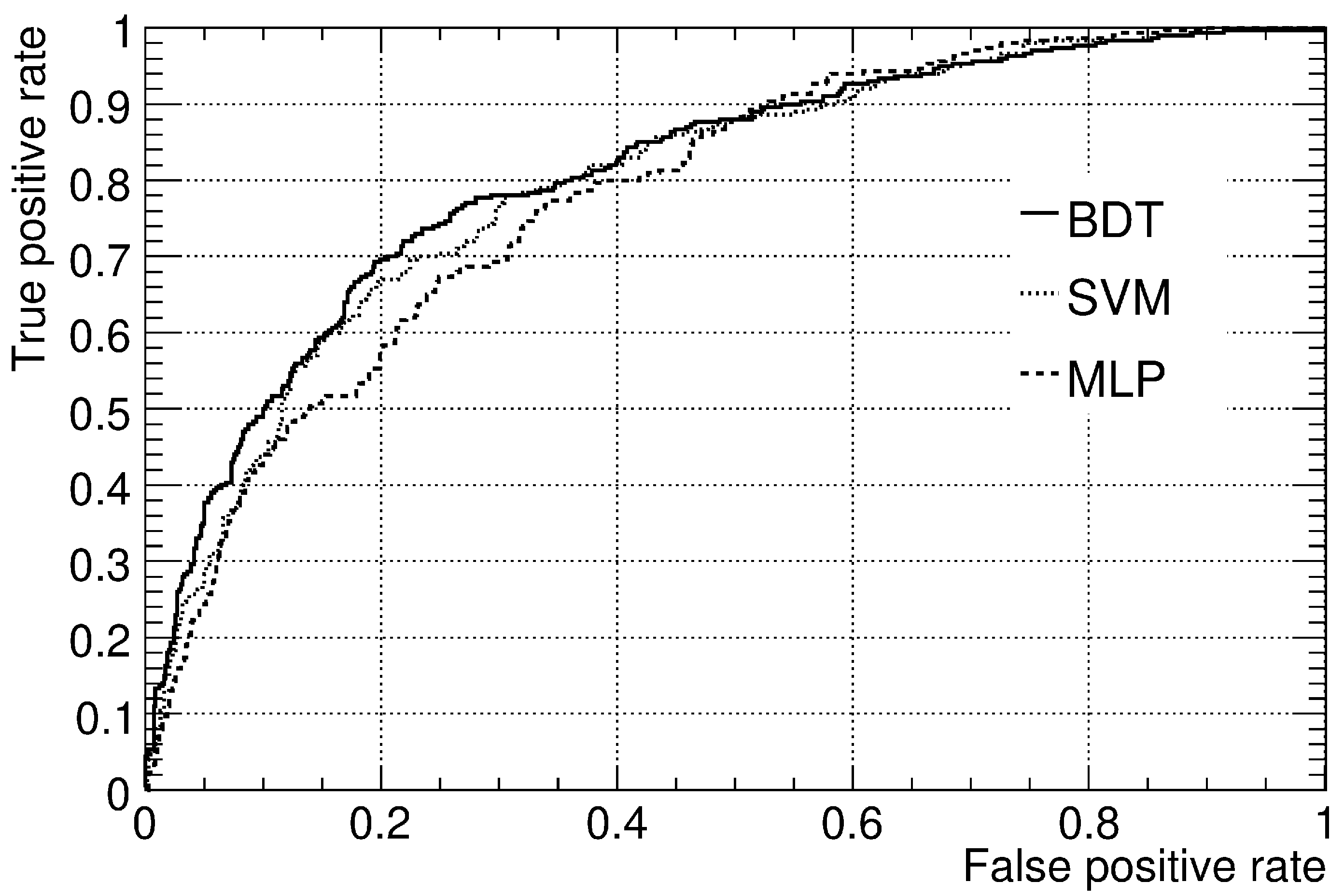
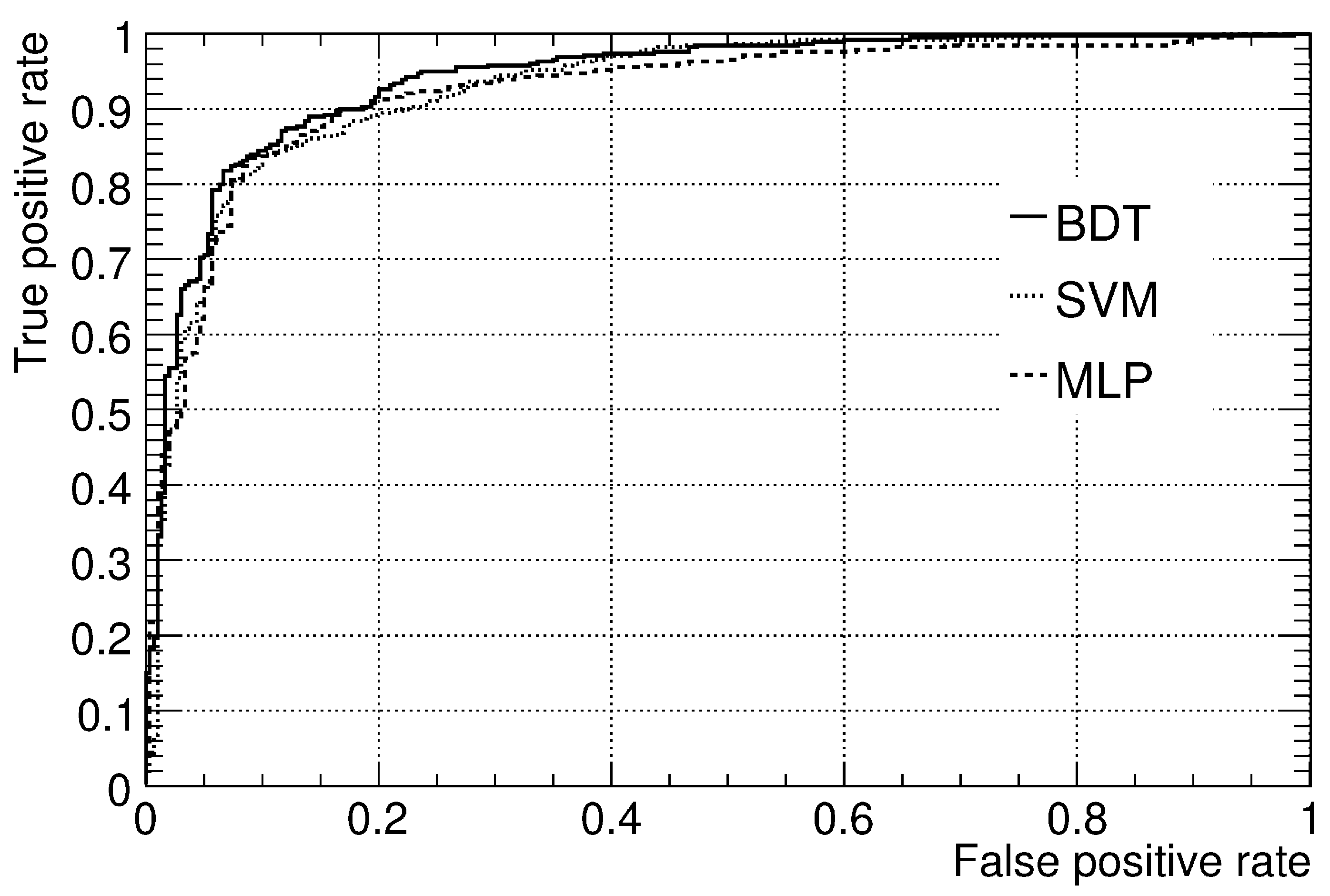
In a pattern classification problem, the data sample is usually divided into a training set and an independent (out-of-sample) test set. The classifier learns the data with the training set, and its predictive power is estimated using the test set. In order to train classifiers with a large fraction of the available data and evaluate the generalization accuracy with the complete dataset, a 10-fold cross-validation was implemented. This technique consists of randomly dividing the dataset into ten mutually exclusive subsets of equal size and, sequentially, testing each of these subsets using the classifier trained on the remaining subsets.

There is no formal theory specifying how to select the optimal hyper-parameters for a given classifier. In practice, the selection of the best set of hyper-parameters is accomplished either by heuristic rules or by “grid-search”. In this approach, different sets of hyper-parameter values are scanned and the set with best predictive performance is selected. The performance of boosted decision trees (BDT) is optimized by adjusting two hyper-parameters: the number of decision trees that are aggregated to form the final classifier and the minimum number of credit applicants that a tree node must contain in order to be split. When the number of applicants in a node reaches this threshold value the growth of the branch is terminated.

The multilayer perceptron (MLP) contained a single hidden layer (a network with a single hidden layer is sufficient to model a complex system to any desired degree of accuracy, provided sufficient hidden nodes are available [33]). The input layer contained a number of nodes equal to the number of attributes in the samples (24 nodes for the German dataset and 14 nodes for the Australian dataset), while the output layer contained a single node. The activation functions of the nodes were sigmoids. The network was trained by error back-propagation using the steepest descent algorithm. Three parameters were optimized: the number of neurons in the hidden layer, the number of epochs, and the learning rate. The support vector machine (SVM) was implemented with a Gaussian radial basis function. Two parameters were optimized: the width of the Gaussian kernel $\sigma$ and the cost parameter C. To find the best pair $(\sigma ,C)$ a grid-search was performed using the recipe in [34], in which these parameters take values from sequences of powers of 2. All models were implemented using the framework provided by the TMVA package [35].

2.3. Results

The performance of credit scoring models is measured in terms of the capability to distinguish the good credit population from the bad credit population in the test sample. As mentioned in Section 1.2, the BDT algorithm assigns to credit applicants a score according to Equation (3). Good credits will typically have large positive scores while bad credits will have large negative scores. Credit applicants with a score above a certain threshold value are granted credit, while the remaining are rejected. For a given cut-off value there are two types of incorrect predictions: the model grants credit to an applicant that will default on the financial obligation (Type I error) and the model rejects credit to an applicant that is creditworthy (Type II error or False Alarm Ratio). The cut-off value represents a compromise between a large efficiency for granting credit and a large rejection of bad credits. An excessively large tendency for granting credit may result in severe economic losses due to delinquent costumers, while a credit policy that is too strict may result in opportunity costs larger than the costs of default. The selected cut-off value will ultimately depend on the relative ratio of the misclassification costs associated with Type I and Type II errors (in general, the costs associated with misclassifying bad applicants are financially more damaging than those associated with misclassifying good applicants).

Since the cut-off value depends on the credit policy of the financial institution, it is convenient to express the performance of the models in terms of the receiver operating characteristics (ROC) curve. The ROC curve is a plot of the true positive rate (proportion of bad credit that are correctly classified) as a function of the false positive rate (Type II error) for the full range of possible cut-off values. Figure 2 and Figure 3 show the ROC curves for the German and Australian credit datasets obtained by merging the 10 cross-validation test sets, respectively. If a model could completely separate the two populations, it would always give correct predictions. In this case, the ROC curve would pass through the point (0,1) and the area under the ROC curve would be equal to 1. On the other hand, a random guess classifier would result in as many correct predictions as incorrect predictions being made. In this case, for any cut-off value, the true positive rate would be on average equal to the false positive rate, and the ROC curve would be a 45 degree straight line intersecting (0,0) and (1,1). A model that performs better than random guessing gives a concave ROC curve above this straight line. The higher the model accuracy, the steeper will the ROC curve be. Therefore, the area under the ROC curve (AUC) is a measure of the generalization accuracy that is independent of the cut-off value.

Table 1. Comparison of the area under the ROC curve for the multilayer perceptron (MLP), support vector machine (SVM), and boosted decision trees (BDT).

Model	German Data	Australian Data
MLP	78.3%	92.3%
SVM	79.9%	92.9%
BDT	81.1%	94.0%

presents the AUC for the three models obtained by trapezoidal integration. For the German dataset the SVM outperformed the MLP, whereas BDT outperformed both the MLP and the SVM. For the Australian dataset a similar ordering of the predictive performance of the three models was observed.

2.4. Comparison of the AUC Estimates

In order to test the statistical significance of the differences between the areas under the ROC curves predicted by the models under consideration, the nonparametric approach introduced in [36] was followed. The AUC can be interpreted as the probability that the score of a randomly selected good credit applicant is higher than that of a randomly selected bad credit applicant. Therefore, denoting by $X_i^{\left(g\right)}$, $i=1,\cdots ,n_g$ the estimated scores for the good credit set and by $X_j^{\left(b\right)}$, $j=1,\cdots ,n_b$ the estimated scores for the bad credit set, an unbiased estimator of the AUC is given by the Wilcoxon–Mann–Whitney statistic:

$$\widehat{\theta }=\frac{1}{n_b{n}_g}\sum _{j=1}^{n_b}\sum _{i=1}^{n_g}{\mathbf{1}}_{X_i^{\left(g\right)}>X_j^{\left(b\right)}},$$

(4)

where the indicator function ${\mathbf{1}}_{X_i^{\left(g\right)}>X_j^{\left(b\right)}}$ is 1 if $X_i^{\left(g\right)}>X_j^{\left(b\right)}$, and 0 otherwise. In order to obtain an estimate of the variance of $\widehat{\theta }$, the structural components of the ith good credit and jth bad credit must be calculated:

$$v(X_i^{\left(g\right)})=\frac{1}{n_b}\sum _{j=1}^{n_b}{\mathbf{1}}_{X_i^{\left(g\right)}>X_j^{\left(b\right)}},v(X_j^{\left(b\right)})=\frac{1}{n_g}\sum _{i=1}^{n_g}{\mathbf{1}}_{X_i^{\left(g\right)}>X_j^{\left(b\right)}}.$$

(5)

Then, an estimator for the variance of $\widehat{\theta }$ can be obtained from:

$$\mathrm{V}\widehat{\mathrm{a}}\mathrm{r}(\widehat{\theta })=\frac{1}{n_g(n_g-1)}\sum _{i=1}^{n_g}{\left[v(X_i^{\left(g\right)})-\widehat{\theta }\right]}^2+\frac{1}{n_b(n_b-1)}\sum _{j=1}^{n_b}{\left[v\left(X_j^{\left(b\right)}\right)-\widehat{\theta }\right]}^2.$$

(6)

In order to compare the AUC of two alternative models, A and B, the covariance of the corresponding AUC estimators must also be obtained:

$$\begin{array}{ccc}\mathrm{C}\widehat{\mathrm{o}}\mathrm{v}({\widehat{\theta }}_A,{\widehat{\theta }}_B)\hfill & =& \frac{1}{n_g(n_g-1)}\sum _{i=1}^{n_g}\left[v_A\left(X_i^{\left(g\right)}\right)-{\widehat{\theta }}_A\right]\left[v_B\left(X_i^{\left(g\right)}\right)-{\widehat{\theta }}_B\right]\\ \hfill & +& \frac{1}{n_b(n_b-1)}\sum _{j=1}^{n_b}\left[v_A\left(X_j^{\left(b\right)}\right)-{\widehat{\theta }}_A\right]\left[v_B\left(X_{Bj}^{\left(b\right)}\right)-{\widehat{\theta }}_B\right].\end{array}$$

(7)

To test the null hypothesis $H_0:{\widehat{\theta }}_A={\widehat{\theta }}_B$ versus the alternative hypothesis $H_1:{\widehat{\theta }}_A\ne {\widehat{\theta }}_B$ the following test statistic is computed:

$$T=\frac{{\left({\widehat{\theta }}_A-{\widehat{\theta }}_B\right)}^2}{\mathrm{V}\widehat{\mathrm{a}}\mathrm{r}({\widehat{\theta }}_A-{\widehat{\theta }}_B)},$$

(8)

where:

$$\mathrm{V}\widehat{\mathrm{a}}\mathrm{r}({\widehat{\theta }}_A-{\widehat{\theta }}_B)=\mathrm{V}\widehat{\mathrm{a}}\mathrm{r}({\widehat{\theta }}_A)+\mathrm{V}\widehat{\mathrm{a}}\mathrm{r}({\widehat{\theta }}_B)-2\mathrm{C}\widehat{\mathrm{o}}\mathrm{v}({\widehat{\theta }}_A,{\widehat{\theta }}_B).$$

(9)

The test statistic T is asymptotically ${\chi }^2$-distributed with one degree of freedom.

Table 2. Statistical test for comparing the area under the ROC curves estimated by the different models.

Test	German Data		Australian Data
	T	p-Value	T	p-Value
MLP – SVM	2.781	0.095	1.132	0.288
MLP – BDT	4.916	0.027	6.778	0.009
SVM – BDT	1.774	0.183	3.737	0.053

shows the results of applying this test to the estimated ROC curves. For both datasets one can reject the null hypothesis $H_0:{\widehat{\theta }}_{BDT}={\widehat{\theta }}_{MLP}$ with a 95% significance level and, therefore, there is strong evidence that the performance of BDT is better than that of the MLP. For the Australian dataset there is also strong evidence that BDT outperformed SVM. However, for the German dataset the difference between these methods was not statistically significant.

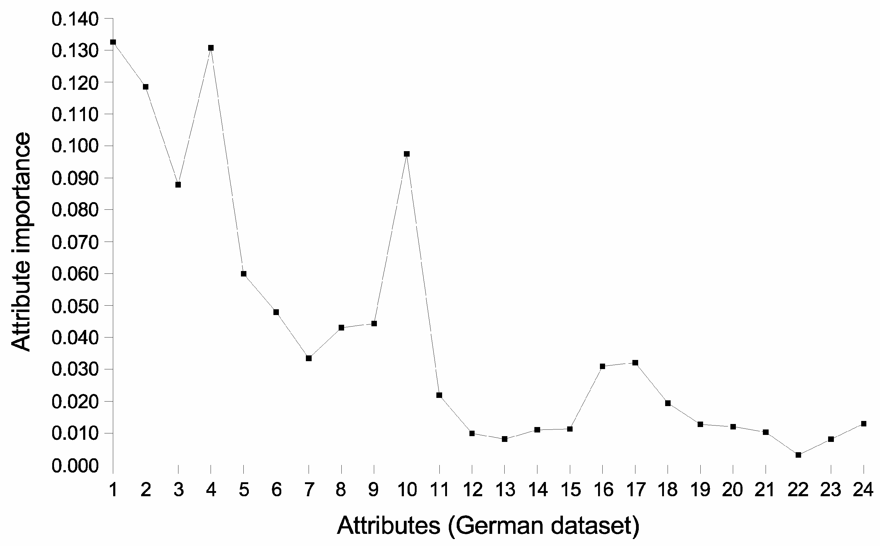
2.5. Relative Importance of the Attributes

Boosted decision trees provide a straightforward and intuitive measure of the relative contribution of the attributes to separate instances according to the target classification. Using this approach, a ranking of the most useful attributes can be established. This ranking is derived by counting the number of times an attribute is employed in the node-splitting procedure and by weighting each split by the separation gain it has accomplished and by the number of instances in the node [29].

Figure 4 shows the relative importance of the attributes for the German credit dataset. The first and fourth attributes are the most important. These attributes correspond to the status of the existing checking accounts and the credit amount, respectively. They are followed by the second attribute (duration of the loan) and the tenth attribute (age of the applicant). Also important is the third attribute, which represents the credit history of the applicant (e.g., if previous credits were paid punctually or there were delays in paying off). The fifth to ninth attributes have moderate importance. They correspond to the status of savings accounts, the employment condition, the marital status and sex, the amount of years living in the present residence, and the property that the applicant owns, respectively. Figure 5 shows the relative importance of the attributes for the Australian credit dataset. The nature of the attributes in this dataset is unknown. In this dataset, the eighth attribute is clearly the most important. Also of note is that the contributions of attributes 1, 11, and 12 are negligible.

3. Conclusions

This paper introduced a credit scoring model of consumer loans using boosted decision trees—a learning technique that allows to combine several decision trees to form a classifier that is obtained from a weighted majority vote of the classifications given by individual trees. The generalization accuracy of boosted decision trees was compared with that of a multilayer perceptron and support vector machines. Boosted decision trees outperformed the multilayer perceptron and the support vector machines on two real-world credit card application datasets. On the basis of these results, it can be concluded that boosted decision trees may be a competitive alternative to these techniques in credit scoring applications. It was also shown that boosted decision trees provide an elegant way to rank the attributes that most significantly affect the likelihood of default.

References

1. Crook, J.N.; Edelman, D.B.; Thomas, L.C. Recent developments in consumer credit risk assessment. Eur. J. Oper. Res. 2007, 183, 1447–1465. [Google Scholar] [CrossRef]
2. West, D. Neural network credit scoring models. Comput. Oper. Res. 2000, 27, 1131–1152. [Google Scholar] [CrossRef]
3. Reichert, A.K.; Cho, C.C.; Wagner, G.M. An examination of the conceptual issues involved in developing credit-scoring models. J. Bus. Econ. Stat. 1983, 1, 101–114. [Google Scholar]
4. Wiginton, J.C. A note on the comparison of logit and discriminant models of consumer credit behavior. J. Financ. Quant. Anal. 1980, 15, 757–770. [Google Scholar] [CrossRef]
5. Henley, W.E.; Hand, D.J. A k-nearest neighbor classifier for assessing consumer risk. Statistician 1996, 44, 77–95. [Google Scholar] [CrossRef]
6. Frydman, H.E.; Altman, E.I.; Kao, D.-L. Introducing recursive partitioning for financial classification: The case of financial distress. J. Financ. 1985, 40, 269–291. [Google Scholar] [CrossRef]
7. Davis, R.H.; Edelman, D.B.; Gammerman, A.J. Machine learning algorithms for credit-card applications. Ima J. Manag. Math. 1992, 4, 43–51. [Google Scholar] [CrossRef]
8. Jensen, H.L. Using neural networks for credit scoring. Manag. Financ. 1992, 18, 15–26. [Google Scholar] [CrossRef]
9. Blanco, A.; Pino-Mejías, R.; Lara, J.; Rayo, S. Credit scoring models for the microfinance industry using neural networks: Evidence from Peru. Expert Syst. Appl. 2013, 40, 356–364. [Google Scholar] [CrossRef]
10. Zhao, Z.; Xu, S.; Kang, B.O.; Kabir, M.M.J.; Liu, Y.; Wasinger, R. Investigation and improvement of multi-layer perceptron neural networks for credit scoring. Expert Syst. Appl. 2015, 42, 3508–3516. [Google Scholar] [CrossRef]
11. Ong, C.-S.; Huang, J.-J.; Tzeng, G.-H. Building credit scoring models using genetic programming. Expert Syst. Appl. 2005, 29, 41–47. [Google Scholar] [CrossRef]
12. Baesens, B.; Van Gestel, T.; Viaene, S.; Stepanova, M.; Suykens, J.; Vanthienen, J. Benchmarking state-of-the-art classification algorithms for credit scoring. J. Oper. Res. Soc. 2003, 54, 1028–1088. [Google Scholar] [CrossRef]
13. Li, S.-T.; Shiue, W.; Huang, M.-H. The evaluation of consumer loans using support vector machines. Expert Syst. Appl. 2006, 30, 772–782. [Google Scholar] [CrossRef]
14. Bellotti, T.; Crook, J. Support vector machines for credit scoring and discovery of significant features. Expert Syst. Appl. 2009, 36, 3302–3308. [Google Scholar] [CrossRef] [Green Version]
15. Harris, T. Credit scoring using the clustered support vector machine. Expert Syst. Appl. 2015, 42, 741–750. [Google Scholar] [CrossRef] [Green Version]
16. Plawiak, P.; Abdar, M.; Acharya, R. Application of new deep genetic cascade ensemble of SVM classifiers to predict the Australian credit scoring. Appl. Soft Comput. 2019, 84, 105740. [Google Scholar] [CrossRef]
17. Lee, T.-S.; Chiu, C.-C.; Lu, C.-J.; Chen, I.-F. Credit scoring using the hybrid neural discriminant technique. Expert Syst. Appl. 2002, 23, 245–254. [Google Scholar] [CrossRef]
18. Hsieh, N.-C. Hybrid mining approach in the design of credit scoring models. Expert Syst. Appl. 2005, 28, 655–665. [Google Scholar] [CrossRef]
19. Lee, T.-S.; Chen, I.-F. A two-stage hybrid credit scoring model using artificial neural networks and multivariate adaptive regression splines. Expert Syst. Appl. 2005, 28, 743–752. [Google Scholar] [CrossRef]
20. Bastos, J.A. Ensemble predictions of recovery rates. J. Financ. Serv. Res. 2014, 46, 177–193. [Google Scholar] [CrossRef]
21. West, D.; Dellana, S.; Qian, J. Neural network ensemble strategies for financial decision applications. Comput. Oper. Res. 2005, 32, 2543–2559. [Google Scholar] [CrossRef]
22. Asuncion, A.; Newman, D.J. UCI Machine Learning Repository. University of California, Irvine, School of Information and Computer Science. Available online: https://archive.ics.uci.edu/ml/index.php (accessed on 4 November 2022).
23. Bastos, J.A. Credit Scoring with Boosted Decision Trees. Mpra Pap. 8034. 2008. Available online: https://mpra.ub.uni-muenchen.de/8034/ (accessed on 5 November 2022).
24. Tsai, C.-F.; Hsu, Y.-F.; Yen, D.C. A comparative study of classifier ensembles for bankruptcy prediction. Appl. Soft Comput. 2014, 24, 977–984. [Google Scholar] [CrossRef]
25. Abellán, J.; Castellano, J.G. A comparative study on base classifiers in ensemble methods for credit scoring. Expert Syst. Appl. 2017, 73, 1–10. [Google Scholar] [CrossRef]
26. Xia, Y.; Liu, C.; Li, Y.Y.; Liu, N. A boosted decision tree approach using Bayesian hyper-parameter optimization for credit scoring. Expert Syst. Appl. 2017, 78, 225–241. [Google Scholar] [CrossRef]
27. Zhou, J.; Li, W.; Wang, J.; Ding, S.; Xia, C. Default prediction in P2P lending from high-dimensional data based on machine learning. Phys. Stat. Mech. Its Appl. 2019, 534, 122370. [Google Scholar] [CrossRef]
28. Liu, W.; Fan, H.; Xia, M. Credit scoring based on tree-enhanced gradient boosting decision trees. Expert Syst. Appl. 2022, 189, 116034. [Google Scholar] [CrossRef]
29. Breiman, L.; Friedman, J.H.; Olshen, R.A.; Stone, C.J. Classification and Regression Trees; Wadworth International Group: Belmont, CA, USA, 1984. [Google Scholar]
30. Freund, Y.; Schapire, R.E. A short introduction to boosting. J. Jpn. Soc. Artif. Intell. 1991, 14, 771–780. [Google Scholar]
31. Schapire, R.E. The boosting approach to machine learning: An overview. Nonlinear Estim. Classif. 2002, 149–173. [Google Scholar]
32. Freund, Y.; Schapire, R.E. Experiments with a new boosting algorithm. In Proceedings of the 13th International Conference on Machine Learning, Bari, Italy, 3–6 July 1996; pp. 148–156. [Google Scholar]
33. Hornik, K.; Stinchcombe, M.; White, H. Multilayer feedforward networks are universal approximators. Neural Netw. 1989, 2, 359–366. [Google Scholar] [CrossRef]
34. Hsu, C.-W.; Chang, C.-C.; Lin, C.-J. A Pratical Guide to Support Vector Classification. 2007. Available online: https://www.google.com.hk/url?sa=t&rct=j&q=&esrc=s&source=web&cd=&ved=2ahUKEwjRiJ3yybT7AhXMklYBHcQfAEQQFnoECBEQAQ&url=https%3A%2F%2Fwww.csie.ntu.edu.tw%2F~cjlin%2Fpapers%2Fguide%2Fguide.pdf&usg=AOvVaw3va31QH9SMVmNquoUoRfdN (accessed on 4 November 2022).
35. Hoecker, A.; Speckmayer, P.; Stelzer, J.; Tegenfeldt, F.; Voss, H.; Voss, K. TMVA—Toolkit for Multivariate Data Analysis. arXiv 2007, arXiv:physics/0703039. [Google Scholar]
36. DeLong, E.; DeLong, D.; Clarke-Pearson, D. Comparing the area under two or more correlated receiver operating characteristic curves: A nonparametric approach. Biometrics 1988, 44, 837–845. [Google Scholar] [CrossRef] [PubMed]
Figure 1. Illustration of a decision tree for credit scoring.
Forecasting 04 00050 g001
Figure 2. Receiver operating characteristics (ROC) curve for the multilayer perceptron (MLP), support vector machine (SVM), and boosted decision trees (BDT), for the German credit dataset.
Forecasting 04 00050 g002
Figure 3. Receiver operating characteristics (ROC) curve for the multilayer perceptron (MLP), support vector machine (SVM) and boosted decision trees (BDT), for the Australian credit dataset.
Forecasting 04 00050 g003
Figure 4. Relative importance of attributes predicted by boosted decision trees for the German dataset.
Forecasting 04 00050 g004
Figure 5. Relative importance of attributes predicted by boosted decision trees for the Australian dataset.
Forecasting 04 00050 g005