Can Groups Improve Expert Economic and Financial Forecasts?

Abstract

Economic and financial forecasts are important for business planning and government policy but are notoriously challenging. We take advantage of recent advances in individual and group judgement, and a data set of economic and financial forecasts compiled over 25 years, consisting of multiple individual and institutional estimates, to test the claim that nominal groups will make more accurate economic and financial forecast than individuals. We validate the forecasts using the subsequent published (real) outcomes, explore the performance of nominal groups against institutions, identify potential superforecasters and discuss the benefits of implementing structured judgment techniques to improve economic and financial forecasts.

1. Introduction

Forecasts are an essential element of economics and finance, influencing corporate investment strategies, public policy priorities and private decisions about expenditure (e.g., [1,2]). They are produced at an enormous range of scales and settings, from global to local and for a multitude of purposes, specific applications and contexts (e.g., [3,4,5]). Forecast inaccuracies may result in costly misallocations of resources by banks [6], sub-optimal or ineffective policy decisions by government, and direct costs to institutional and private investors [7].

Many financial and media institutions publish economic and financial forecasts and have done so for decades. Some are based on detailed economic models updated regularly by government economists; others are based on the intuitions of independent economic experts.

There have been many assessments of the accuracies of institutional forecasts (e.g., comparing the Reserve Bank of New Zealand to external forecasts [8], and assessing the accuracy of the forecasts from the Michigan Quarterly Econometric Model [9]). The Australian Treasury regularly reviews its forecast performance including reviews in 2005, 2012, 2015 and an externally sourced review in 2017 that focused primarily on macroeconomic models [10]. The most recent review of forecast accuracy by the Australian Treasury found its forecasts to be unbiased but, like most forecasters, to have a poor record predicting economic turning points [11]. The Australian Treasury produces confidence ranges on their major forecasts (published in Budget Paper 2, Statement 7 each year), along with sensitivity analysis on the impact on the budget on changes in economic parameters. Despite many such periodic reviews and institutional assessments, the authors of [12] claim there is a continuing need for more prudent forecasts and thorough validation in many contexts.

It has been known for some time that subjective judgement influences both model-based and unstructured forecasts [13]. In the 1980s, Tetlock and colleagues began asking experts to make a suite of geopolitical forecasts. Their prescient experiments discovered that few economic forecasts were accurate, and many were indistinguishable from random error [14]. The authors of [12] commented that, “despite major advances in evidence-based forecasting methods, forecasting practice in many fields has failed to improve over the past half-century.”

Through a government-sponsored forecasting tournament, the authors of [15,16] identified the phenomenon that some individuals are much better at making geopolitical forecasts than others. The authors of [17] documented similar phenomena amongst experts in nuclear safety, earth science, chemical toxicity and space shuttle safety. Importantly, ref. [18] documented that when such people are organised into interacting groups, they make even more accurate geopolitical predictions (cf. [19]). However, the potential for groups to make better economic and financial forecasts remains relatively untested.

The authors of [18] noted that the ability to make good judgements does not correlate with attributes conventionally associated with predictive performance such as qualifications, years of experience or status in the field. The lack of an association between expert status and performance has been documented in other disciplines [20]. Adding to this complexity, past performance in predicting financial outcomes is a poor indicator of future performance, but pooling independent forecasts can substantially improve forecast accuracy [21]. Thus, the accuracy of public and private economic and financial forecasts in many domains remains an open question.

Performance weights have been proposed as a way of improving collective (group or crowd-based) forecasts and there is a substantial literature that discusses alternatives and documents performance gains when using test questions to weight performance [17]. Nevertheless, equally weighed judgements often perform well compared to a number of approaches to weighting, because while they are not fully optimal, they are almost always better than individual forecasts and they are likely in many circumstances to be nearly optimal [22].

In this study, we compile a large set of economic forecasts made over 25 years by Australian media outlets and government agencies and use them to evaluate whether nominal groups provide more accurate economic and financial forecasts than do individuals. We validate judgements against published outcomes. We evaluate the performance of official government and media-based forecasts. We compare the performance of forecasters based in different kinds of workplaces, the accuracy of judgements based on different question types, and discuss the potential for economic and financial superforecasting. We examine whether forecast accuracy improved over the 25 years since 1990. Finally, we discuss the potential for building on these results and improving economic and financial forecasts through the deployment of structured elicitation techniques.

2. Methods

2.1. Data

The Fairfax Business Day survey of economists (for an example survey see: https://www.petermartin.com.au/2016/06/midyear-scope-survey-low-rates-weak.html, last accessed in 2020) has been running twice a year for more than 25 years and is published in both the Sydney Morning Herald and The Age newspapers in Australia. Our data set includes a total of 37 surveys: two surveys per year (January and July) starting January 1996, finishing July 2016. In each survey between 20 and 28 economists were asked between 20 and 26 questions.

The set has some missing data. The original publications of several surveys, specifically, July 2002, July 2011 and July 2012 were unobtainable or the data they contained was not discernible in the available copies. Amongst those surveys that were available, we were not able to analyze the data for every question for every survey as the answers were sometimes illegible. In other cases, the questions or the experts’ answers were ambiguous, and the outcome could not be definitely determined. These cases were omitted. There were 117 unique questions in the data set that were repeated in multiple surveys (see Appendix A for the full list of questions). There was a total of 701 questions and 14,860 expert forecasts. The same question asked in a different month (i.e., July vs January) was scored as a different question. Thus, each six-month forecast of GDP asked in January was considered a different question from the equivalent six-month GDP forecast asked in July of the same year. Different forecast lengths for the same statistic were also treated as different questions. We grouped the related questions by subject (see

Table 1. The number of forecasts of different kinds appearing in the Fairfax Business Day survey of economists appearing between January 1996 and July 2016 and the corresponding forecasts made by Treasury.

Subject	No. of Survey Forecasts	No. of Treasury Forecasts	Subject Code
Australian GDP	1418	36	11
Private consumption	246	7	12
Housing investment	538	12	13
Total domestic demand	379	8	14
Net exports	375	7	15
CPI	445	11	21
Unemployment	566	14	23
Employment growth	289	7	24
WPI	417	9	25
Budget balance	931	38	26
Terms of trade	380	7	27
Net foreign debt	645	0	28
Current account deficit	327	7	29
Reserve Bank cash rate	1220	0	31
90 Day bank bills	609	0	32
10 year bonds	869	0	33
All Ords Index	253	0	35
S&P/ASX 200	400	0	36
Size and direction of next RBA move	78	0	37
S&P/ASX 500	72	0	38
Dow Jones	41	0	43
FTSE 100	102	0	44
Nikkei 225	111	0	45
$AU in Usc	1059	0	51
$AU in YEN	600	0	52
$AU in Euro c	481	0	53
$AU in Trade Weighted Index (TWI)	381	0	54
OECD GDP growth	162	5	61
US GDP growth	377	15	62
Japan GDP growth	299	12	63
China GDP growth	271	12	64
World GDP growth	519	22	65
TOTAL	14,860	229

).

One of the “experts” in this set was the Australian Department of The Treasury (hereafter Treasury). Its forecasts were designed primarily to focus on providing a clear macroeconomic outlook for policy (spending and tax) decisions and to set the budget: the most important parameters are GDP, CPI, wages and employment growth, and company profits. The Treasury does not provide some estimates such as the exchange rate and official interest rates because such forecasts could be controversial and may themselves influence the outcome.

We examined the performance of Treasury estimates against the other expert forecasts and against the actual outcomes. The published July expert forecasts were compared to the budget forecasts issued in May, and the January forecasts were compared to Treasury’s Mid-Year Economic and Fiscal Outlook published in December. Thus, the survey respondents had access to slightly more information than those involved in the Treasury forecasts. We tested the importance of differences in the timing of estimates by comparing the accuracy of forecasts made one month and six months apart.

Forecasts were assessed by comparing the quantitative estimates with the actual outcomes (methods for comparison are described below). Outcomes were drawn from the sources representing the authoritative source to which each expert referred when making their forecasts (

Table 2. Data sources (last accessed in 2020) for verification of each of the forecasts outcomes.

GDP Australia financial year	Australian Federal budget (1997–2018) ${}^1$
GDP Trading partners (calendar)	Australian Federal budget (1997–2018) ${}^1$
Private investment	Australian Federal budget (1997–2018) ${}^1$
CPI	Australian Federal budget (1997–2018) ${}^1$
Average earnings	Australian Federal budget (1997–2018) ${}^1$
Unemployment	Australian Federal budget (1997–2018) ${}^1$
Net foreign debt	Australian Bureau of Statistics Series 5302 ${}^2$
Current account balance	Australian Federal budget (1997–2018) ${}^1$
Terms of trade	Australian Federal budget (1997–2018) ${}^1$
90 Day bank bills	Reserve Bank of Australia ${}^3$
10 Year Government bonds	Reserve Bank of Australia ${}^3$
Reserve bank target interest rate	Reserve Bank of Australia ${}^3$
Exchange rates	Reserve Bank of Australia ${}^3$
S&P/ASX 200	Google finance 1996–2001 ${}^4$, ASX 2002–2016 ${}^5$
All Ords	Google finance 1996–2001 ${}^4$, ASX 2002–2016 ${}^5$

¹https://archive.budget.gov.au/; ²https://www.abs.gov.au/ausstats/[email protected]/mf/5302.0; ³https://rba.gov.au/statistics/historical-data.html; ⁴https://www.google.com/finance; ⁵https://www.asx.com.au/about/historical-market-statistics.htm#End_of_month_values.

).

A total of 154 different experts contributed forecasts in these data. The experts appearing in the Fairfax Business Day survey were usually presented as belonging to a particular industry (

Table 3. The number of experts with different affiliations and the number of forecasts they contributed in these data.

Industry Group	No. of Forecasts	No. of Experts
Financial	6599	38
University	2116	15
Industry group	1595	10
Consultant	1375	9
Other	819	5
Treasury	229	1
Missing	2356	77
TOTAL	15,089	155

). Some surveys did not identify an industry affiliation for all experts and for some, industry affiliations were not readily discernible from the information provided, resulting in 2585 missing data points.

Before analysing the data detailed in this section, it is worth mentioning that the Fairfax Business Day survey of economists was not conducted for making group forecasts, and was not conducted within the framework of a structured elicitation protocol (which often prescribes a way of evaluating the forecasts). As a consequence, the breath of the possible analyses is limited.

2.2. Analysis

A loss function is an objective function that evaluates forecast accuracy. Several are used routinely including quadratic loss functions for point predictions (equivalent to the mean squared error (MSE)) and scoring rules such as the Brier score for probabilistic forecasts [23]. The authors of [24] provided a review of different families of measures for assessing point estimate, with a particular focus on the measures used in time series forecasting. The mean square error (MSE) and root mean square error (RMSE) have been popular historically largely due to their analogues in statistical modelling [24]. We used three of the standard measures of forecast accuracy, each of which has somewhat different properties; the Mean Absolute Percentage Error (MAPE), the Average Log-Ratio Error (ALRE), and the Symmetric Median Absolute Percentage Error (SMdAPE), although we report only ALRE and SMdAPE here because MAPE provided no useful additional insights. For a more complete analysis and comparisons of these measures we refer the reader to [25]. Ideally, either the measures used in the analysis of expert elicited data are specified prior to the elicitation, or the elicitation questions are formulated to suit the chosen measures [26]. Unfortunately neither of the two situations occurred when planning the collection of the elicited data analysed here.

The experts provided only point estimates (for continuous response variables only) for each forecast; that is, they did not provide credible intervals or other measures of uncertainty around their estimates. Evaluation metrics for point estimates measure error as the difference between a prediction r and the observed value x. In general, percentage errors are preferred to absolute errors because of their scale independence, which allows comparisons. Absolute error is simply:

$$e_n=\left|r_n-x_n\right|.$$

(1)

where $r_n$ is the forecast/prediction and $x_n$ is the outcome/observed value of the $n^{th}$ variable, and absolute percentage error is:

$$p_n=\frac{100e_n}{x_n}.$$

(2)

The Mean Absolute Percentage Error (MAPE) gives the average percentage difference between a prediction and the observed value (when N predictions are evaluated)

$$\mathrm{MAPE}=\frac{1}{N}\sum _{n=1}^N{p}_n.$$

(3)

Calculating MAPE is perhaps the simplest approach to (scale/range) standardisation. A disadvantage is that this measure rewards forecasts that are below the outcome value compared to forecasts that are above, generating a bias in accuracy assessments [27]. The formula for MAPE is not symmetric in the sense that interchanging $x_n$ and $r_n$ does not lead to the same answer, despite the fact that the absolute error is the same before and after the switch, because switching the denominator leads to a different result [27].

Symmetric percentage errors compensate for the inherent bias in MAPE by dividing by the arithmetic mean of the actual and the forecasted value (see p. 348 of [28]). The symmetric median absolute percentage error (SMdAPE) is:

$$\mathrm{SMdAPE}=median\left(200|\frac{e_n}{r_n+x_n}|\right)$$

(4)

However, this measure is susceptible to inflation when values are close to zero. Range coding allows comparisons across different scales. Each response is standardized by the range of responses for that question. Expressing each response $r_i^{{}^{\prime }n}$ for expert i on question n in range coded form gives:

$$r_i^n=\frac{r_i^{{}^{\prime }n}-r_{min}^{{}^{\prime }n}}{r_{max}^{{}^{\prime }n}-r_{min}^{{}^{\prime }n}}$$

(5)

where $r_i^n$ is the range coded response, $r_{max}^{{}^{\prime }n}$ is the maximum of all the responses assessed for question including the true value), and is the minimum of all the responses assessed for question (including the true value). Using the range coded responses, the average log-ratio error (ALRE) is [20]:

$${\mathrm{ALRE}}_i=\frac{1}{N}\sum _{n=1}^N{log}_{10}\left(\frac{x^n+1}{r_i^n+1}\right)$$

(6)

where where N is the total number of questions, $r_i^n$ is the standardized prediction and $x^n$ is the standardized observed (true) value.

ALRE is a relative measure, scale invariant, and emphasizes order of magnitude errors, rather than linear errors. Smaller ALRE scores indicate more accurate responses. For any given question the log ratio scores have a maximum possible value of $0.31$ (corresponding to ${log}_{10}\left(2\right)$), which occurs when the true answer coincides with either the group minimum or group maximum.

As with other scoring metrics, problems arise with the ALRE in certain circumstances. Firstly, for variables for which all participants estimate the correct response it will not be possible to calculate range-coded scores. Secondly, outliers may affect scores in undesirable ways. A single outlier response will lead to the remaining respondents being scored quite highly and close together (i.e., close to zero), and this scaling relative to an outlier may partially mask the skill of the best performers on this question (i.e., lead to its down-weighting), relative to performance on other questions.

2.3. Specific Issues

As noted above, the Treasury makes economic forecasts routinely and these are used as the basis for a wide range of policy decisions. Thus, in the results below, we highlight the performance of the Treasury forecasts against those made by individual experts appearing in the Fairfax Business Day survey. The performance is measured using the two accuracy measures for continuous responses described in Section 2.2. We avoid using more sophisticated measures (e.g., like the ones proposed in [26]) simply because the data itself, and the data collection process do not allow for it.

Similarly, as noted above, it is well established that group judgments routinely out-perform individual judgements, in a wide range of circumstances. Thus, we are interested in comparing the aggregated judgement of a group of forecasters with individual forecasts, and with the Treasury forecasts. We create a nominal group by combining individual economic forecasts based on the simple average of the independent forecasts for each question in each year.

The suite of questions can be broken down into subsets, each of which represents a specific domain of economic forecasting. These categories are shown in

Table 4. The 17 categories (sub-domains) of questions addressed by the experts within three broad domains.

Domain	Sub-Domain (Codes)	No. of Questions
Domain 1	Australian GDP (11)	36
	Private consumption (12)	7
	Housing investment (13)	12
	Total domestic demand (14)	8
	Net exports(15)	7
Domain 2	CPI (21)	11
	Unemployment (23)	14
	Employment growth (24)	7
	WPI (25)	9
	Budget balance (26)	38
	Terms of trade (27)	7
	Current account deficit (29)	7
Domain 6	OECD GPD Growth (61)	5
	US GPD Growth (62)	15
	Japan GPD Growth (63)	12
	China GPD Growth (64)	12
	World GPD Growth (65)	22

(a subset of the categories in Table 1).

In this study, we had the opportunity to use performance on questions answered earlier in the assessment period to weight judgements subsequently, and to update dynamically when people joined or left the expert pool or answered a subset of the questions. We developed an iterative approach to performance weighting to implement this (see Appendix A).

Using differential weighting when aggregating judgements, rather than simple averages (which correspond to equal weighting), is a mathematical aggregation technique often used in expert judgement. However, it is considered best practice for such weights to be informed only by prior performance on similar tasks [29]. The number of questions each expert answers varies, hence, so does their performance and their corresponding weight. To identify and eliminate some of the randomness in the weights we estimate them both on a yearly basis, and cumulatively (using all questions answered up to a certain point). Ideally, more variations on what answers we use for calculating the weights and how far ahead predictions can be evaluated for accuracy should be investigated. Unfortunately the dataset size does not allow for these variations.

Finally, it is worth mentioning the strong analogies between model averaging and the mathematical aggregation of expert predictions. In the framework of statistical learning modelling, the performance of pooled models improves that of individual models [30], and this is also true for the mathematical aggregation of expert predictions. Moreover, Bayesian model averaging allows weighting different features of the model proportionally to their statistical importance [31], much like weighting expert predictions proportionally to the experts’ performance. However, the types of problems assessed by the statistical learning models and the size of the datasets used to calibrate these models are very different than their analogue in the expert elicited data context.

3. Results

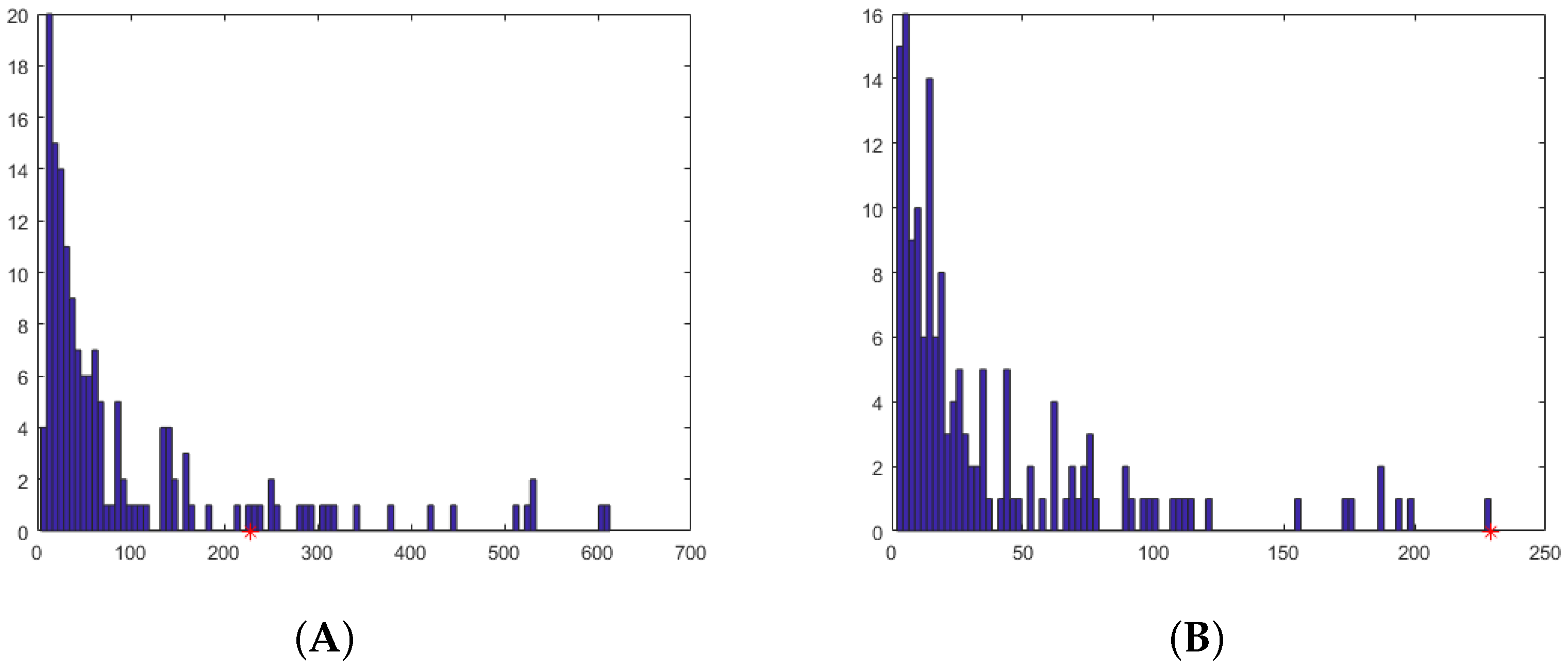
Some experts answered many more questions than others (Figure 1A). 113 experts answered 100 or fewer questions in total over the period 1996 to 2016. The Australian Treasury answered a subset of 229 questions and Figure 1A shows the frequency of expert responses to that subset of questions. The majority of experts answered less than half of the full set of questions.

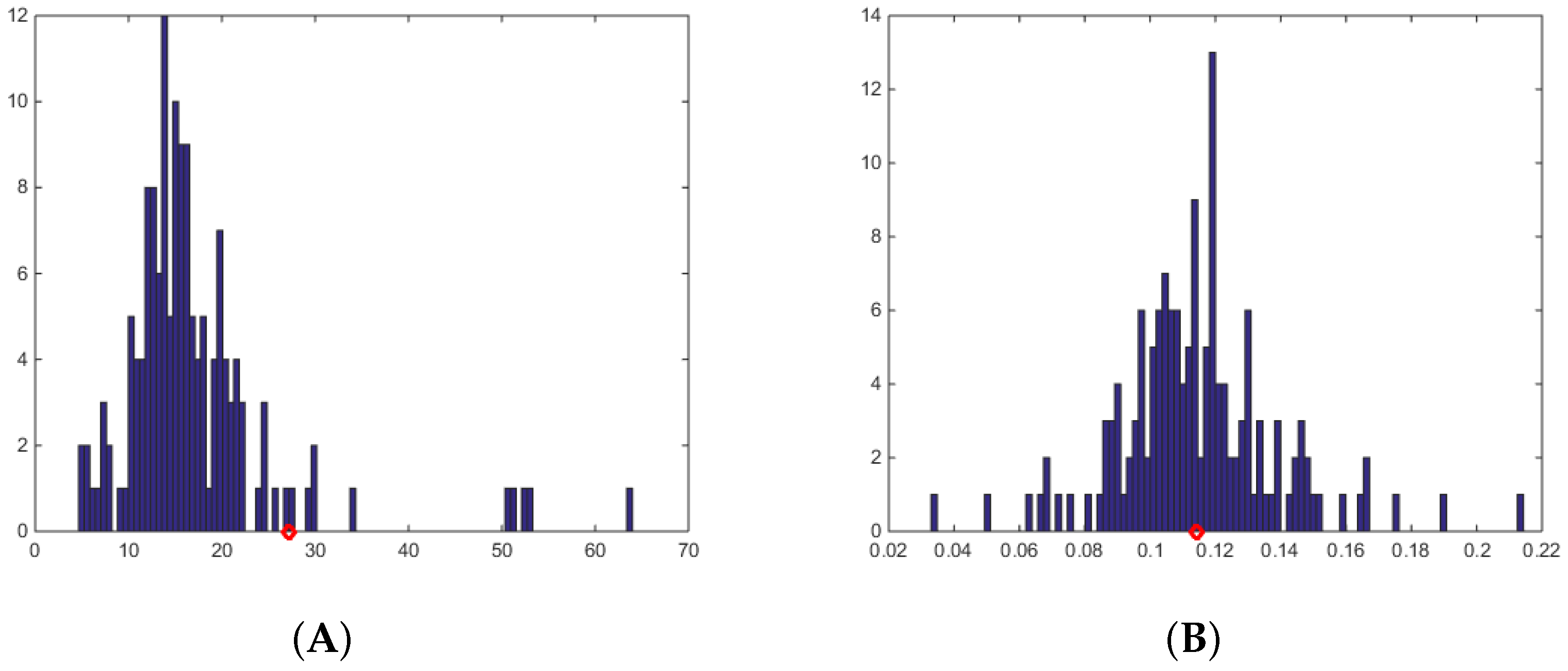
Figure 2 displays the histograms of the average errors in economic forecasts made by all experts for all questions between 1996 and 2016.SMdAPE is simple (linear) ratio and displays a typical right skew. ALRE is a log-ratio and is more or less symmetrical around the midpoint.

We noted above that the Treasury “expert” has a slight disadvantage because it predicts one to two months earlier (over periods of one or two months longer) than the other experts. To test the importance of this difference, we compared the accuracy of predictions made over six and 12 months. The results (not shown) indicate that there was no appreciable deterioration in the accuracy of forecasts. Accuracy of forecasts was similar, irrespective of the period over which the predictions were made. The 1–2 month difference between Treasury and the other experts will not have affected the qualitative outcomes outlined below.

As noted above, the two measures used here tell slightly different stories. In the following two tables we consider the 10 best and 10 worst performers according to the different measures, when calculated for the experts who answered questions in at least three years (this is equivalent, for most experts, to answering more than 50 questions). We expect the measures to be fairly reliable when calculated from a large set of questions. Some interesting patterns emerge. Five experts (numbers 96, 59, 137, 21 and 44) appear amongst the top 10 under both measures (

Table 5. The accuracy of the 10 best performers who answered questions in at least three years, under two accuracy measures. For ALRE which is an average score we can calculate the 90% confidence intervals. For SMdAPE, which is a median, we report the 5^th and the 95^th percentiles forming the 90% credible interval. We denote both credible and confidence intervals by CI.

Expert No.	SMdAPE	CI for SMdAPE	Expert No.	ALRE	CI for ALRE
96	8.95	(0, 89.52)	96	0.079	(0.06, 0.09)
59	9.52	(0, 113.36)	115	0.081	(0.06, 0.1)
137	10.17	(0.56, 74.52)	59	0.082	(0.06, 0.1)
95	11.10	(0, 68.76)	44	0.089	(0.07, 0.11)
125	11.28	(0.97, 161.31)	45	0.095	(0.08, 0.11)
21	11.75	(0.29, 152.47)	137	0.095	(0.08, 0.11)
1	11.76	(0, 206.90)	21	0.097	(0.09, 0.14)
44	11.98	(0.32, 83.66)	107	0.097	(0.09, 0.12)
64	12.44	(0.04, 216.85)	98	0.100	(0.082, 0.11)
112	12.54	(0.64, 296.97)	22	0.103	(0.1, 0.11)

).

When considering the 10 worst performers under each measure (

Table 6. The accuracy of the 10 worst performers who answered questions in at least three years, under two accuracy measures. For ALRE which is an average score we can calculate the 90% confidence intervals. For SMdAPE, which is a median, we report the 5^th and the 95^th percentiles forming the 90% credible interval. We denote both credible and confidence intervals by CI. Expert 999 is the Australian Treasury forecast.

Expert No.	SMdAPE	CI for SMdAPE	Expert No.	ALRE	CI for ALRE
33	19.88	(1.15, 317.6)	24	0.128	(0.111, 0.137)
106	20.51	(1.04, 339.2)	1	0.129	(0.104, 0.145)
49	20.56	(1.43, 366.4)	41	0.13	(0.103, 0.150)
147	20.84	(0.15, 173.6)	33	0.13	(0.124, 0.138)
41	21.54	(0.29, 366.3)	73	0.13	(0.114, 0.142)
102	22.22	(1.89, 340)	79	0.137	(0.112, 0.146)
63	23.50	(1.21, 269.6)	102	0.19	(0.118, 0.144)
999	24	(1.98, 512.1)	49	0.142	(0.127, 0.148)
103	26.62	(0.28, 192.1)	82	0.144	(0.132, 0.153)
82	29.16	(0.90, 430.7)	103	0.162	(0.152, 0.173)

), five experts (numbers 33, 41, 102, 103, 82) appear under both measures. The Treasury (expert 999) is amongst the worst performers under SMdAPE.

It is interesting to note that amongst the best performers, none answered questions in 2008, whereas amongst the worst performers, half of them did. In general, the worst performers answered questions in more years than did the best performers, exposing themselves to more difficult and more diverse situations.

If we exclude the questions from 2008, the best scores do not change much (since none of the best performers answered questions in 2008). For the set of worst scores, seven out of ten remain unchanged for ALRE and half remain the same for SMdAPE. If, on the other hand, we look at only those experts who answered questions in 2008 (among other years), only 21 experts and the Treasury gave estimates in at least three years, including 2008. Out of these, only one expert is among the best five performers on both scores (and this expert is not in any of the previous subsets) and interestingly the Treasury scores among the best on ALRE (0.11) and among the worst on SMdAPE (229).

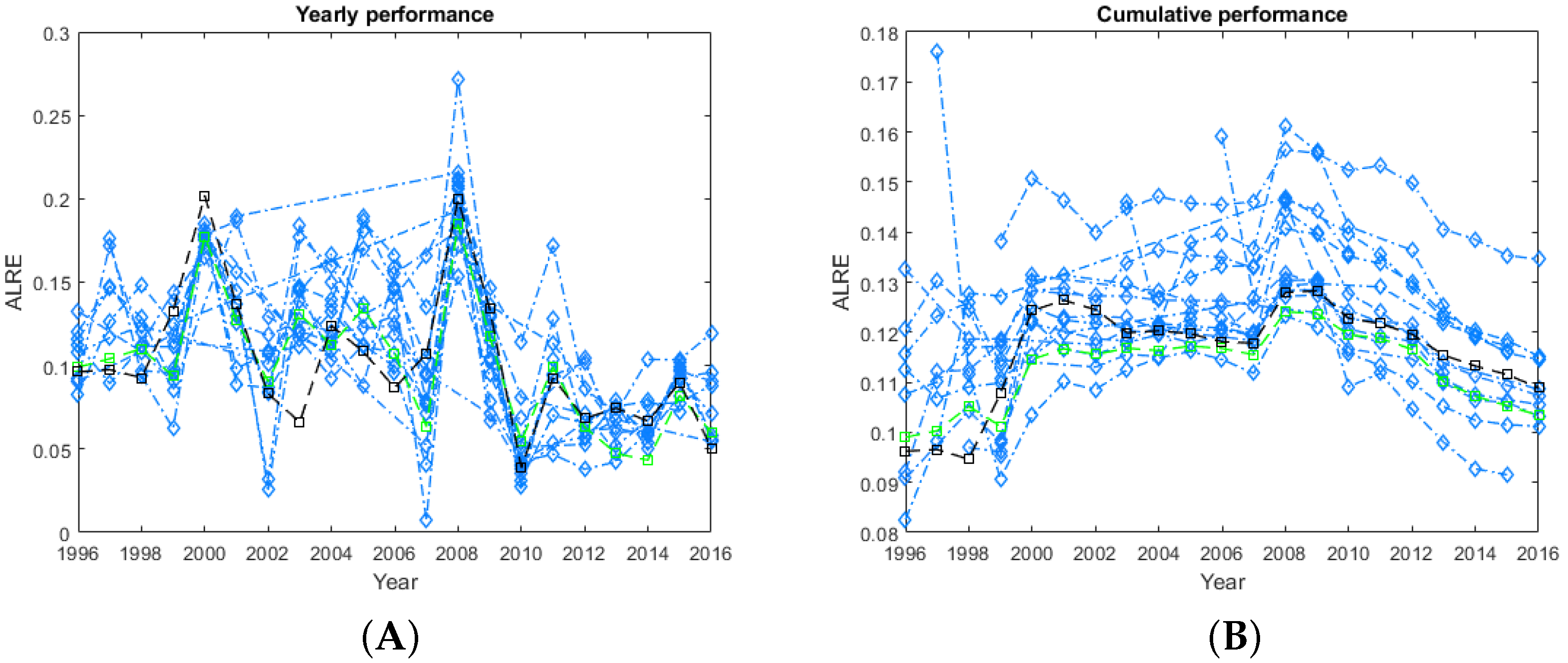
Figure 3A shows the average ALRE scores for experts who answered at least one question per year, for at least 10 out of the 25 years. In some years, expert forecasts were appreciably worse than in others (particularly for the years 2000 and 2008). The Australian Treasury forecasts are not appreciably better than the performance of individual experts over the same period.

Another way of looking at these data is to use all the questions answered prior to a particular year and to calculate ALRE from all previously answered questions, in a cumulative manner. Figure 3B shows the cumulative performance of these experts over the same period.

Restricting average ALRE performance to the subset of 229 questions that were answered by the Treasury provides a more direct assessment of the relative performance of Treasury forecasts, albeit at the expense of some power (Figure 4).

A relatively small number of individual experts outperform the Treasury forecasts when the set is restricted to the questions answered by the Treasury and by individual experts. However, there are two important features in these results. First, one expert consistently outperformed the treasury, over many questions and many years of making forecasts. Second, the nominal group composed of the average forecasts (an equally weighed combination of forecasts) of the individual experts consistently outperformed the Treasury forecasts.

Again, restricting the questions to those answered by the Treasury and by individual experts, in nine out of the 17 sub-domains of economic forecasting outlined above, the Treasury forecast was better than the combined experts’ forecasts. In eight cases, the equally weighted forecast was better. In three out of these eight, the performance weighted forecast was better than both. However, the differences were modest and in no case were they statistically significantly different (see Figure 5).

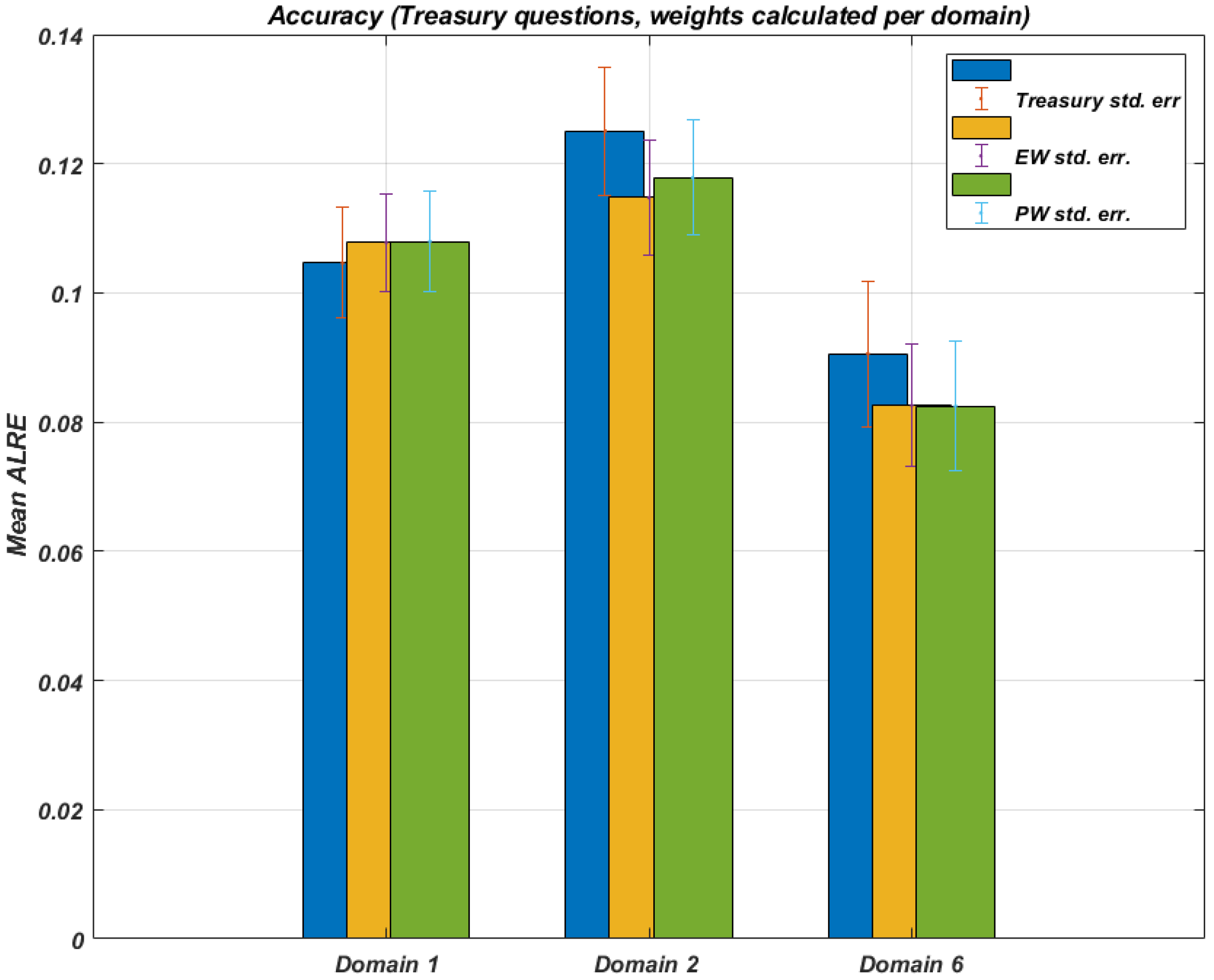
When the questions are grouped into the three broad domains noted in Table 4, Treasury forecasts are somewhat better in ’Domain 1’ (Australian economic growth), but less accurate than the performance weighted aggregation or the equally weighted aggregation estimates in ’Domains 2’ (Australian macro-economic indicators) and ’Domain 6’ (OECD and other country economic growth) (see Figure 6).

If instead we calculate performance weights for experts based on all the questions they answered rather than only the subset that coincides with the Treasury answers, the situation changes slightly. Both the performance weighted aggregation and the equally weighted aggregations provides more accurate predictions than Treasury, with the difference in performance being significant for ’Domain 2’ ( see Figure 7).

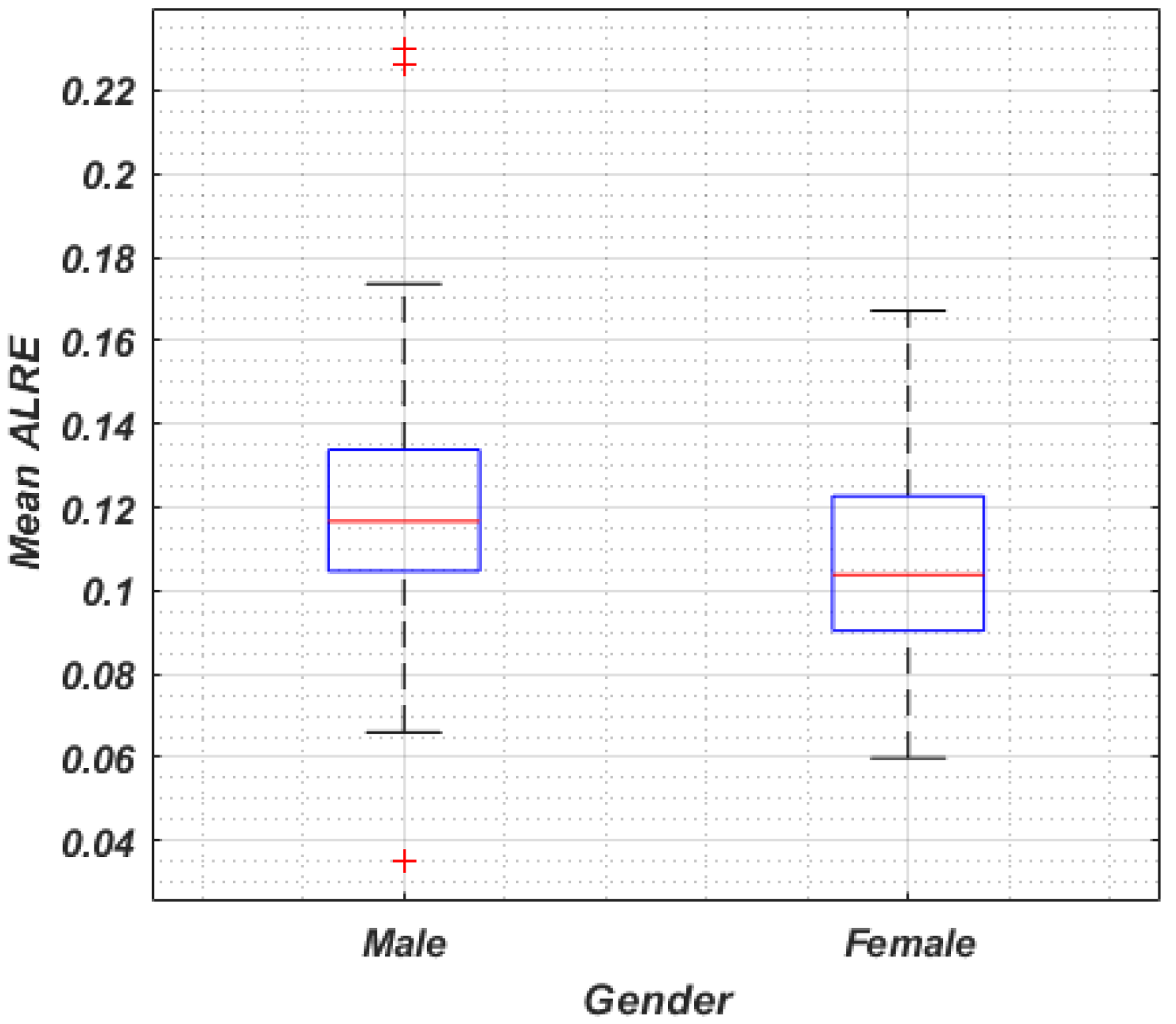
There is some evidence that the attributes of individuals may provide a guide to the performance of individual forecasters [14]. This group of experts contained 17 women and 130 men (not all experts specified their gender). We examined the question of performance related to gender in these economic forecasts by equalizing the number of women and men, selecting random groups of male respondents from the available pool, constraining the questions so that the same subset of questions was addressed by each group, and calculating the average ALRE per group (see Figure 8). On average, female respondents provided slightly more accurate forecasts than their male counterparts. This result may be confounded by other variables including the participants’ ages, expertise, and other demographic attributes.

4. Discussion

Economic forecasts are the basis for many government and industry policies and decisions at all levels in all jurisdictions including monetary policy. Some are model-based, some use multiple models, and some are subjective judgements made by individuals, using unspecified data sources and algorithms. Recent extensions use machine-learning algorithms [32]. However, irrespective of the platform or approach, the ideologies, methods and contexts of the forecasters can influence economic forecast accuracies substantially [33]. Such influences are difficult to anticipate in any individual or group [14,34].

As noted in the introduction, the primary motivation for this work was to test whether the phenomena observed in other domains, namely that nominal groups make more accurate forecasts, hold for important economic and financial parameters. Our results illustrate that there are appreciable benefits to be gained from amalgamating a number of independent judgements for complex economic and financial forecasts. In most circumstances, the average (equally weighed aggregation) of a group of independent forecasts should perform reliably and effectively.

It is interesting to note that one individual in the group performed extremely well. In any weighting scheme, the weight afforded to their judgements would have exceeded those of the other participants. Such superforecasters, when placed in a group together with other high-performing individuals, can produce group forecasts that do better than any of the high-performing individuals [35].

Our results indicate that errors are correlated in time. Since the significant shift in economic variables in 2008, there is evidence that forecast accuracy has improved consistently since then. The ALRE scores for most participants, including the Treasury and the nominal group improve noticeably between 2009 and 2016 (see Figure 3B and Figure 4B). As noted above, none of the best performers answered questions in 2008. Arguably, one of the most valuable attributes of a forecaster is to forecast the timing and magnitude of a turning point. Such an analysis would require a longer data set than even the one provided here, but it is an important topic for future research.

Motivational bias may also constrain some forecasts; financial analysts may not make a controversial forecast involving a large downturn if it could damage their business. When economic and financial conditions shift abruptly and unexpectedly, as they did in 2000 and 2008, then all predictions tend to be error prone. Other studies have shown that economic surprises are in themselves unsurprising [36]; that is, we should prepare for surprises. We also know that financial executives are routinely and persistently overconfident; their 80% confidence intervals enclose realized market returns only 36% of the time [37].

The implicit importance of some of the forecasts in the set of questions is considerably higher than others. Thus, we may expect more effort and more careful reasoning to emerge in some question sets than in others. For instance, the GDP forecast is a critical element of economic policy development and a small (say 1%) difference is important. In contrast, a financial sector forecast such as stockmarket outcomes of plus or minus 10% are not unusual. Importantly, the performance of the Treasury forecasts is indeed slightly better on GDP forecasts.

It is important to note that The Fairfax Business Day survey of economists was not conducted for the purpose of making group forecasts. The benefits of group judgement emerge here from the simplest of constructions, namely, nominal groups composed of equally weighted, independent judgements. There are a number of alternatives approaches to judgements of uncertain parameters and events, so-called structured expert judgements, that take advantage of group dynamics and interactions to further improve judgements [38,39]. They involve independent initial assessments, facilitated discussions to resolve context and meaning and to share relevant information, revision of estimates, and the subsequent generation of combined, weighted or unweighted, forecasts [40]. Despite the fact that structured expert judgement techniques were not used in this analysis, the group expert performance was comparable to that of Treasury. Deploying structured expert judgement techniques at critical phases of the process would have improved the accuracy of the group forecasts [19], likely leading them to consistently outperform those of the Treasury.

These results imply that the Treasury forecasts made over the period of this study would have benefited from greater diversity and group judgment. Treasury forecasts are an amalgam of advice from Commonwealth and State departments, banks, industry groups, individual experts, the OECD and others. The assessments are also unpinned by economic models. The author of [11], in reviewing the forecasting capability of the Australian Treasury, noted its reliance on model-based forecasts and the need to expand the range of inputs and views into its forecast process. Thus, the issue may not be one of diversity per se, but rather, of ensuring that the method for eliciting and combining expert judgements is disciplined and structured, to avoid the biases and psychological pitfalls that can derail individual and group assessments made informally [19].

References

1. Elliott, G.; Timmermann, A. Economic forecasting. J. Econ. Lit. 2008, 46, 3–56. [Google Scholar] [CrossRef]
2. Deloitte Access Economics. Long Term Economic Scenario Forecasts; Australian Energy Market Operator: Melbourne, Australia, 2019. [Google Scholar]
3. Altshuler, C.; Holland, D.; Pingfan, H.; Li, H. The World Economic Forecasting Model at the United Nations; Department of Economic and Social Affairs: New York, NY, USA, 2016. [Google Scholar]
4. Wang, Q.; Martinez-Anido, C.; Wu, H.; Florita, A.; Hodge, B. Quantifying the economic and grid reliability impacts of improved wind power forecasting. IEEE Trans. Sustain. Energy 2016, 7, 1525–1537. [Google Scholar] [CrossRef]
5. Rickman, D. Regional Science Research and the Practice of Regional Economic Forecasting: Less Is Not More. In Regional Research Frontiers-Vol. 1; Jackson, R., Schaeffer, P., Eds.; Springer: Cham, Switzerland, 2017; pp. 135–149. [Google Scholar]
6. Kupiec, P. A regulatory stress test to-do list: Transparency and accuracy. J. Risk Manag. Financ. Inst. 2018, 11, 132–147. [Google Scholar]
7. Perez, R.; Schlemmer, J.; Hemker, K.; Kivalov, S.; Kankiewicz, A.; Dise, J. Solar energy forecast validation for extended areas & economic impact of forecast accuracy. In Proceedings of the 43rd Photovoltaic Specialists Conference (PVSC), Portland, OR, USA, 5–10 June 2016; Jackson, R., Schaeffer, P., Eds.; IEEE: Manhattan, NY, USA, 2016; pp. 1119–1124. [Google Scholar]
8. Labbe, F.; Pepper, H. Assessing recent external forecasts. Reserve Bank N. Z. Bull. 2009, 74, 19–25. [Google Scholar]
9. Donihue, M. Evaluating the role judgment plays in forecast accuracy. J. Forecast. 1993, 12, 81–92. [Google Scholar] [CrossRef]
10. Murphy, C. Review of Economic Modelling at The Treasury, Report ot the Australian Department of the Treasury; Independent Economics; ANU: Canberra, Australia, 2017. [Google Scholar]
11. Tease, W. Review of Treasury’s Macroeconomic Forecasting Capabilities; Independent Economics; ANU: Canberra, Australia, 2015. [Google Scholar]
12. Armstrong, J.; Green, K.; Graefe, A. Golden Rule of Forecasting: Be Conservative. J. Bus. Res. 2015, 68, 1717–1731. [Google Scholar] [CrossRef] [Green Version]
13. Hafer, R.; Hein, S.; MacDonald, S. Market and Survey Forecasts of the Three-Month Treasury-Bill Rate. J. Bus. 1992, 65, 123–138. [Google Scholar] [CrossRef]
14. Tetlock, P. Expert Political Judgment: How Good Is It? How Can We Know? Princeton University Press: Princeton, NJ, USA, 2005. [Google Scholar]
15. Tetlock, P.; Mellers, B.; Rohrbaugh, N.; Chen, E. Forecasting Tournaments: Tools for Increasing Transparency and Improving the Quality of Debate. Curr. Dir. Psychol. Sci. 2014, 23, 290–295. [Google Scholar] [CrossRef]
16. Mellers, M.; Stone, E.; Murray, T.; Minster, A.; Rohrbaugh, N.; Bishop, M.; Chen, E.; Baker, J.; Hou, Y.; Horowitz, M.; et al. Identifying and Cultivating Superforecasters as a Method of Improving Probabilistic Predictions. Perspect. Psychol. Sci. 2015, 10, 267–281. [Google Scholar] [CrossRef]
17. Fifteen years of expert judgement at TUDelft. Saf. Sci. 2008, 46, 234–244. [CrossRef]
18. Mellers, B.; Tetlock, P. From discipline-centered rivalries to solution-centered science: Producing better probability estimates for policy makers. Am. Psychol. 2019, 74, 290–300. [Google Scholar] [CrossRef] [PubMed]
19. Hemming, V.; Burgman, M.; Hanea, A.; McBride, M.; Wintle, B. A practical guide to structured expert elicitation using the IDEA protocol. Methods Ecol. Evol. 2018, 9, 169–180. [Google Scholar] [CrossRef] [Green Version]
20. Burgman, M.; McBride, M.; Ashton, R.; Speirs-Bridge, A.; Flander, L.; Wintle, B.; Fidler, F.; Rumpff, L.; Twardy, C. Expert Status and Performance. PLoS ONE 2011, 6, e22998. [Google Scholar] [CrossRef] [PubMed]
21. Harvey, C.; Liu, Y. Detecting Repeatable Performance. Rev. Financ. Stud. 2018, 31, 2499–2552. [Google Scholar] [CrossRef]
22. Diebold, F.; Shin, M. Beating the Simple Average: Egalitarian Lasso for Combining Economic Forecasts; Penn Institute for Economic Research: Philadelphia, PA, USA, 2017. [Google Scholar]
23. Elliott, G.; Timmermann, A. Economic Forecasting; Number 10740 in Economics Books; Princeton University Press: Princeton, NJ, USA, 2016. [Google Scholar]
24. Hyndman, R.; Koehler, A. Another look at measures of forecast accuracy. Int. J. Forecast. 2006, 22, 679–688. [Google Scholar] [CrossRef] [Green Version]
25. McBride, M. Expert Knowledge for Conservation: Tools for Enhancing the Quality of Expert Judgment. Ph.D. Thesis, University of Melbourne, Parkville, VIC, Australia, 2015. [Google Scholar]
26. Gneiting, T. Making and Evaluating Point Forecasts. J. Am. Stat. Assoc. 2011, 106, 746–762. [Google Scholar] [CrossRef] [Green Version]
27. Tofallis, C. A better measure of relative prediction accuracy for model selection and model estimation. J. Oper. Res. Soc. 2015, 66, 524. [Google Scholar] [CrossRef] [Green Version]
28. Armstrong, J.S. Long-Range Forecasting: From Crystal Ball to Computer; Wiley: Hoboken, NJ, USA, 1978. [Google Scholar]
29. Hanea, A.; Hemming, V.; Nane, G. Uncertainty Quantification with Experts: Present Status and Research Needs. Risk Analysis 2022, 42, 254–263. [Google Scholar] [CrossRef]
30. Hastie, T.; Tibshirani, R.; Friedman, J. The Elements of Statistical Learning; Springer Series in Statistics; Springer Inc.: New York, NY, USA, 2001. [Google Scholar]
31. Giudici, P.; Mezzetti, M.; Muliere, P. Mixtures of products of Dirichlet processes for variable selection in survival analysis. J. Stat. Plan. Inference 2003, 111, 101–115. [Google Scholar] [CrossRef]
32. Ericsson, N.R.; Martinez, A.B. Evaluating Government Budget Forecasts. In The Palgrave Handbook of Government Budget Forecasting; Springer: Berlin/Heidelberg, Germany, 2019; pp. 37–69. [Google Scholar]
33. Bathcelor, R.; Dua, P. Forecaster ideology, forecasting technique, and the accuracy of economic forecasts. Int. J. Forecast. 1990, 6, 3–10. [Google Scholar] [CrossRef]
34. Burgman, M. Trusting Judgements: How to Get the Best out of Experts; Cambridge University Press: Cambrigde, UK, 2015. [Google Scholar]
35. Tetlock, P.; Gardner, D. Superforecasting: The Art and Science of Prediction; Random House: Manhattan, NY, USA, 2016. [Google Scholar]
36. Felix, L.; Kräussl, R.; Stork, P. Predictable Biases in Macroeconomic Forecasts and Their Impact across Asset Classes; CFS Working Paper Series 596; Center for Financial Studies (CFS): Frankfurt am Main, Germany, 2018. [Google Scholar]
37. Ben-David, I.; Graham, J.; Harvey, C. Managerial Miscalibration. Q. J. Econ. 2013, 128, 1547–1584. [Google Scholar] [CrossRef]
38. Cooke, R. Experts in Uncertainty: Opinion and Subjective Probability in Science; Oxford University Press: Oxford, UK, 1991. [Google Scholar]
39. O’Hagan, A. Expert Knowledge Elicitation: Subjective but Scientific. Am. Stat. 2019, 73, 69–81. [Google Scholar] [CrossRef] [Green Version]
40. Hanea, A.; McBride, M.; Burgman, M.; Wintle, B. Classical meets modern in the IDEA protocol for structured expert judgement. J. Risk Res. 2018, 21, 417–433. [Google Scholar] [CrossRef] [Green Version]
Figure 1. The distribution of the number of questions answered by each expert: (A) The frequency of forecasts per expert for all questions, and (B) The frequency of forecasts per expert for restricted to the 229 questions answered by the Australian Treasury.
Forecasting 04 00038 g001
Figure 2. Distributions of errors for expert economic predictions between 1996 and 2016, appearing in the Fairfax Business Day survey of economists: (A) SMdAPE, and (B) ALRE. The Australian Treasury forecasts are indicated by the red dot.
Forecasting 04 00038 g002
Figure 3. The average ALRE scores over all questions, for each year between 1996 and 2016, for all experts who answered at least one question per year for 10 years, shown as (A) yearly performance, and (B) as cumulative performance. Each line corresponds to a single expert, with the black line corresponding to the Australian Treasury forecasts.
Forecasting 04 00038 g003
Figure 4. The average ALRE scores over all questions, for each year between 1996 and 2016, for all experts who answered at least one question from the 229 questions also answered by the Australian Treasury, shown as (A) yearly performance, and (B) as cumulative performance. Each line corresponds to a single expert, with the black line corresponding to the Australian Treasury forecasts. The green line corresponds to the nominal group.
Forecasting 04 00038 g004
Figure 5. Comparative performance of treasury forecasts, the performance weighted (PW), and the equally weighted (EW), a.k.a.nominal group forecast for each of the 17 economic forecasts domain. The figure shows the mean ALRE of forecasts and standard error intervals.
Forecasting 04 00038 g005
Figure 6. Accuracy of Treasury forecasts compared to EW and PW forecasts, with weights calculated only based on the questions answered by Treasury. The figure shows the mean ALRE of forecasts and standard error intervals. Domain 1 = Australian economic growth, Domain 2 = Australian Macro-economic indicators, Domain 6 = OECD and other country economic growth.
Forecasting 04 00038 g006
Figure 7. Accuracy of Treasury forecasts compared to EW and PW forecasts, with weights calculated based on all questions answered by experts. The figure shows the mean ALRE of forecasts and standard error intervals. Domain 1 = Australian economic growth, Domain 2 = Australian Macro-economic indicators, Domain 6 = OECD and other country economic growth.
Forecasting 04 00038 g007
Figure 8. The relative performance of male and female experts in making economic forecasts. The Y–axis range was cropped to make the differences more visible.
Forecasting 04 00038 g008