Abstract
Electrical load forecasting study is required in electric power systems for different applications with respect to the specific time horizon, such as optimal operations, grid stability, Demand Side Management (DSM) and long-term strategic planning. In this context, machine learning and data analytics models represent a valuable tool to cope with the intrinsic complexity and especially design future demand-side advanced services. The main novelty in this paper is that the combination of a Recurrent Neural Network (RNN) and Principal Component Analysis (PCA) techniques is proposed to improve the forecasting capability of the hourly load on an electric power substation. A historical dataset of measured loads related to a 33/11 kV MV substation is considered in India as a case study, in order to properly validate the designed method. Based on the presented numerical results, the proposed approach proved itself to accurately predict loads with a reduced dimensionality of input data, thus minimizing the overall computational effort.
1. Introduction
Nowadays, the energy system is facing a radical revolution towards a green transition, with increasing penetration of renewable energy sources (RES), migration to distributed systems, with new actors like prosumers, and storage integration, both utility scale and domestic, which represent a key technology to decouple energy production and consumption [1].
In this regard, distributed sensor architectures, digital technology, data analytics and computational tools would represent crucial enabling technologies for monitoring, forecasting and maintenance purposes, to better manage the balance between power demand and supply, and to improve embedding of distributed RES; additionally, for the particular case of stand-alone hybrid systems, energy forecasting will particularly help anticipating customers’ behavior, sizing the electrical infrastructure and improving overall system reliability [2]. Therefore, forecasting capability brings helpful insights for security of energy supply, supporting power companies in providing their end-users with advanced demand-side services, and safe and stable systems.
Utility companies have several advantages with accurate load forecasting, such as reduced operation and maintenance costs, optimized management of demand supply, increased system reliability, effective long-term strategic planning for future investments [3,4]. Electrical load forecasting can be generally divided into four main categories based on forecasting time, such as very short-term, short-term [5], medium-term and long-term load forecasting [6]. Load forecasting with different applications with respect to the specific time horizon, such as optimal operations [7], grid stability [8], Demand Side Management (DSM) [9] or long-term strategic planning [10].
On the other hand, with respect to short-term load forecasting, energy trading is another important task for utilities to successfully increase revenues on the day-ahead energy market models. Power wholesale markets have around the world many different mechanisms and day-ahead or infra-day sessions, e.g., in India two categories exist based on trading time, such as Hourly Ahead Market (HAM) and Day Ahead Market (DAM). In HAM, one hour before the time of energy use, energy trading will be open. Similarly, for DAM, one day before the time of energy use, energy can be traded [11].
A methodology was developed for short-Term load forecasting by combining Light Gradient Boosting Machine (LGBM), eXtreme Gradient Boosting machine (XGB) and Multi-Layer Perceptron (MLP) models in [12]. In this hybrid model both XGB-LGBM combining is used for meta-data generation. A multi-temporal-spatial-scale temporal convolutional network was used in [13] to predict active power load. The multi-temporal-spatial-scale technique is used to minimize noise in load data. A hybrid clustering-based deep learning methodology was developed in [14] for short-term load forecasting. Clustering technique was used to make different clusters of distribution transformers based on load profile. Markov-chain mixture distribution model is developed in [15] to predict the load of residential customers by 30 min ahead. A study was done for load forecasting using various machine learning models like SVM, Random Forest and LSTM [16] both individually and with a fusion prediction approach. Short-Term load forecasting was done using convolutional neural networks (CNN) and sequence models like LSTM and GRU in [17]. CNN was used for feature extraction and sequence models are used for load forecasting. A CNN and Deep Residual Network based machine learning model was developed in [18] for short-Term load forecasting. Various regression models along with correlation concept for dimensionality reduction were used for load forecasting in [19]. LSTM and factor analysis based deep learning model was developed in [20] for load foresting within a smart cities environment. Artificial neural network based machine learning models were developed both for photovoltaic power forecasting [21], and load forecasting on MV distribution networks [22]. Most of the papers on probabilistic renewable generation forecasting literature over the last ten years or so have focused on different variants of statistical and machine learning approaches: in [23] a comparison of non-parametric approaches to this probabilistic forecasting problem has been performed. All these methodologies in literature contributed significantly to face short-term electric power load forecasting problems. In order to improve the forecasting accuracy and also to build a light weight model for active power load forecasting applied to a 33/11 kV substation, a new approach was developed in this paper by using recurrent neural networks for load forecasting and Principal Component Analysis for dimensional reduction.
The novelty of the proposed approach consists in a hybrid approach combining the heterogeneous input structure with PCA: in particular, the new approach considers the temporal impact of the previous three hours data and three days at the same hour data, and the previous three weeks at the same hour data, thus enabling the model to predict load with good accuracy by properly capturing temporal resolution diversity (e.g., the weekends load pattern); additionally, PCA is able to extract the most essential features from the given nine input information, thus compacting the input layer and reducing computational load, maintaining the same overall accuracy. The combination of RNN and PCA is used for the first time in short-term load forecasting problem. RNN models were trained using self adaptive Adam optimizer as shown in [24]. Complete literature summary on short-term load forecasting domain with various machine learning approaches is presented in Table 1. All these methodologies provides valuable contribution towards short-term load forecasting but have some limitations like model complexity, accuracy and weekly impact not considered. In this paper, accuracy in load prediction is improved by tuning the RNN model parameters, model complexity reduced by using principle component analysis and weekly impact considered by using features like , and .

Table 1.
Literature summary.
2. Methodology
2.1. Dimensionality Reduction Using Principal Component Analysis (PCA)
Principal Component Analysis (PCA) uses the extraction features approach to compress the original dataset to a lower subspace feature, with the aim of maintaining most of the relevant information. Detailed procedure for most relevant feature extraction using PCA is drawn from [25].
2.2. Recurrent Neural Network (RNN)
The Recurrent Neural Network (RNN) is a network where the activation status of each hidden neuron for the previous input is used to calculate the activation status of the hidden neuron for the current input [26]. The main and most important feature of RNN is the Hidden state, which recalls some information about previous samples. This work produced four distinct models of RNN i.e., RNN-HAM-Model1 (RHM-1), RNN-HAM-Model2 (RHM-2), RNN-DAM-Model1 (RDM-1) and RNN-DAM-Model2 (RDM-2) to forecast power for effective energy trading in Hourly Ahead Market(HAM) and Day Ahead Market (DAM).
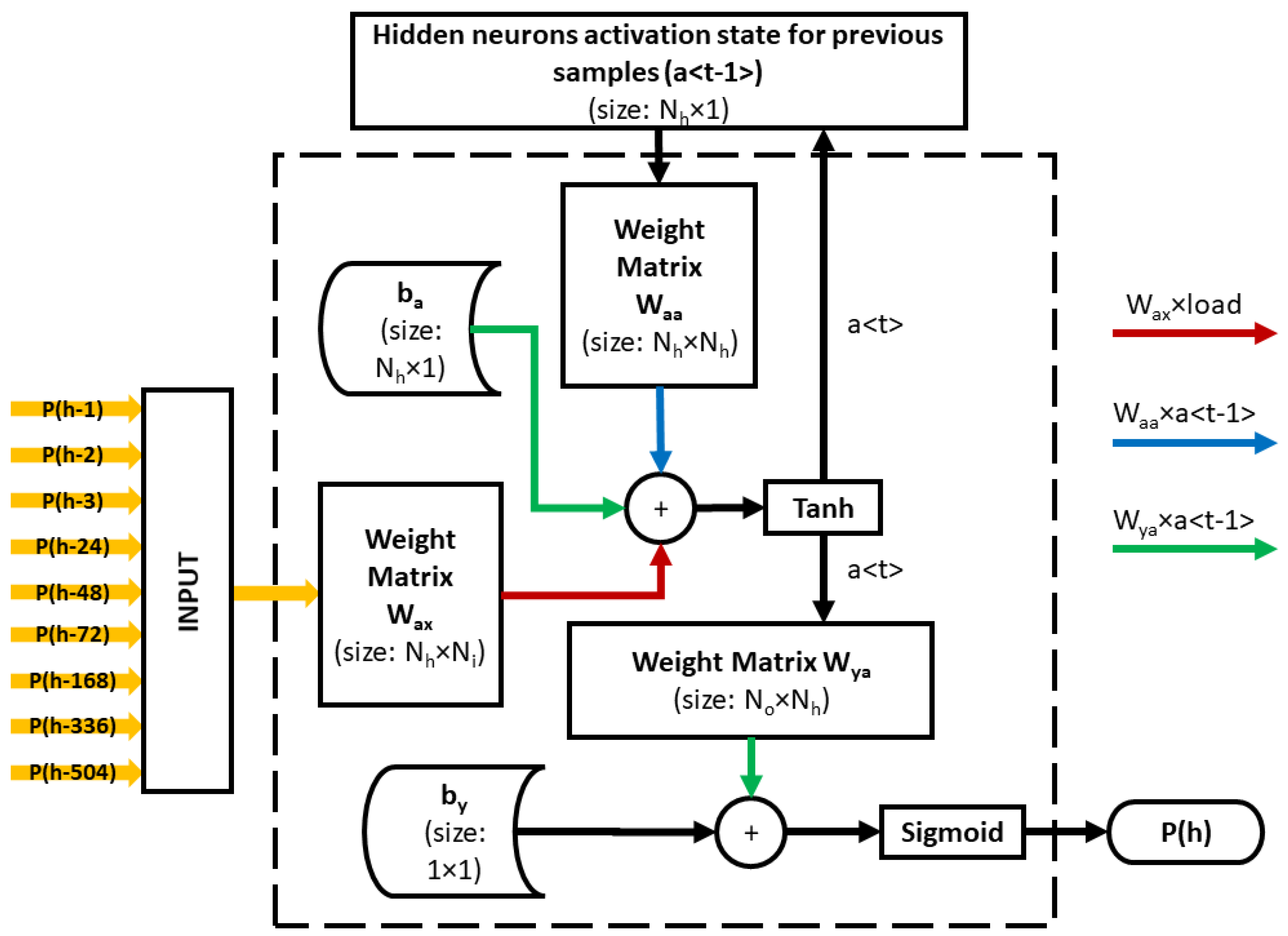
In this study, RHM-1 is designed to predict the load based on the last three hours of load, load at the same time for the last three days and loading at the same time but for the last three weeks. The architecture for the proposed RNN model is shown in Figure 1.

Figure 1.
The considered architecture.
The PCA algorithm is applied to the input features of the load dataset to find the principal components. It has been observed from the CEVR that six principal components cover almost 90% of the load dataset variance. Thus, the 9 input features i.e., , , , , , , , and in each dataset sample are replaced by the corresponding six principal components. These six principal components were used to train the RHM-2. RHM-2 was therefore designed with six input neurons and one output neuron. The architecture of the proposed RNN model is the same as shown in Figure 1, where the number of inputs () is reduced to 6 by the PCA.
RDM-1 is designed to predict the load based on load at the time of forecasting for the last three days and load at forecast time but for the last three weeks. The architecture for the proposed RNN model is the same as shown in Figure 1, where only six input features are considered, i.e., , , , , and , thus .
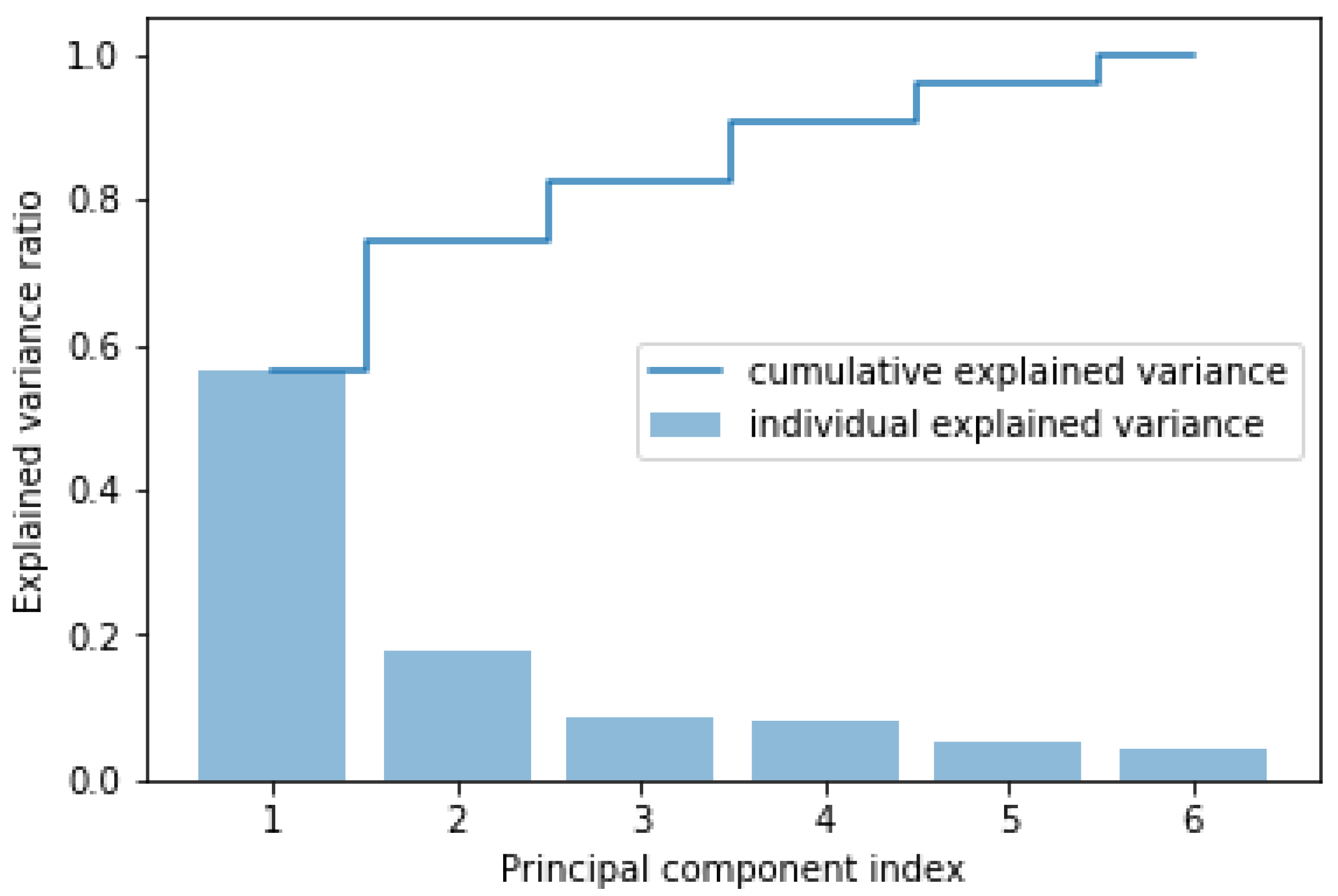
The PCA algorithm is applied to the input features of the load dataset to find the principal components. Load dataset consists in total of 6 input features i.e., , , , , and , and one output feature . It has been observed from CEVR that four principal components cover almost 90% of the load dataset variance. Thus, six input features, i.e., , , , , and for each dataset sample, are converted into four principal components. These four principal components were used to train the RDM-2. RDM-2 was therefore designed with four input neurons and one output neuron. The architecture of the proposed RNN model is the same as shown in Figure 1, where the is finally reduced to 4 by the PCA. Table 2 resumes all this information about the analyzed RNN models, with respect to the considered architecture.

Table 2.
Summary of the RNN models.
Trained RNN model can predict based on input (X) features using Equations (1) and (2). Performance of the all these RNN models have been observed in terms of error metrics like Mean Square Error (MSE), Mean Absolute Error (MAE) and Root Mean Square Error (RMSE) [27] as shown in Equations (3)–(5), respectively.
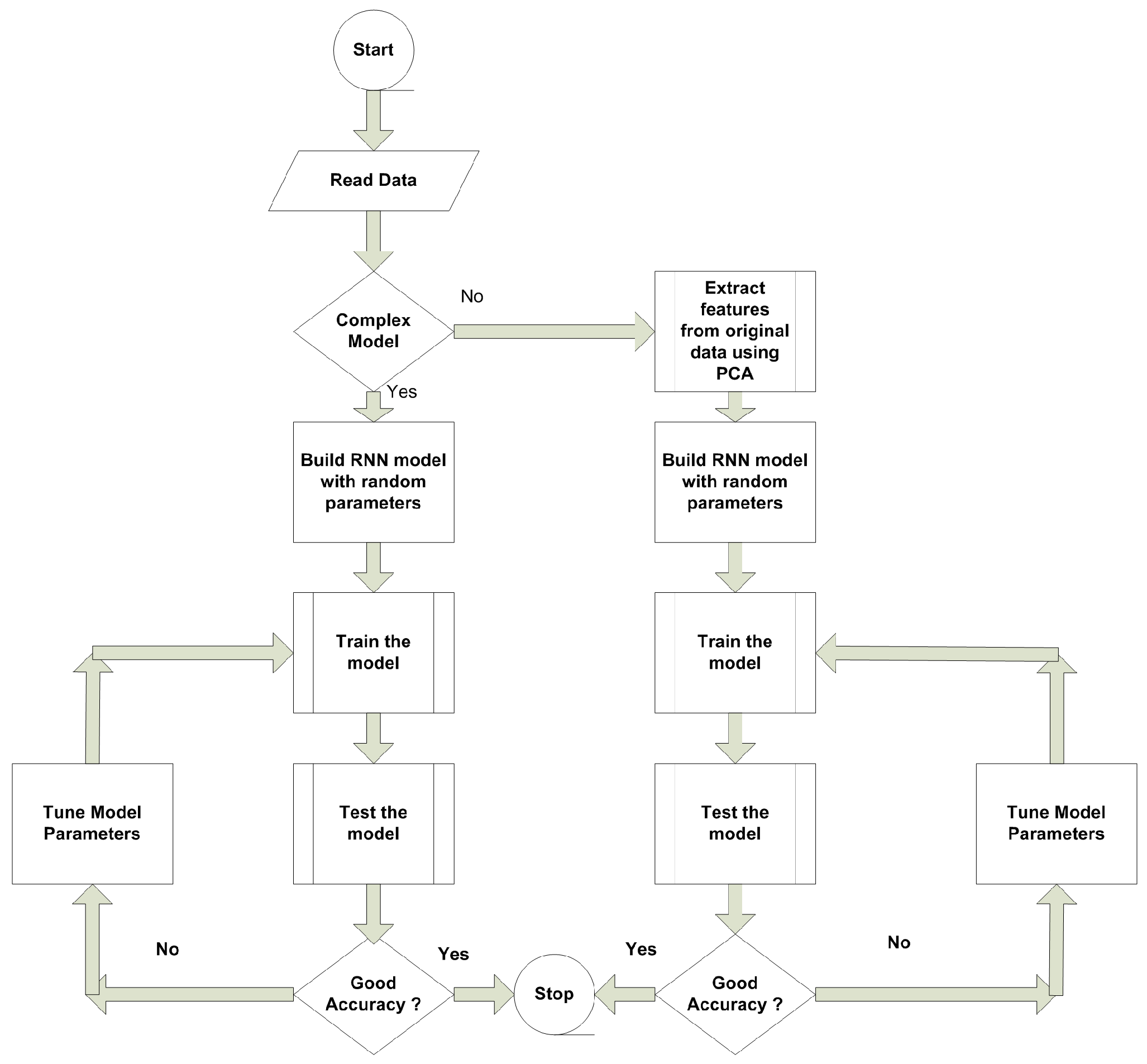
The complete work done in this paper is presented in Figure 2.
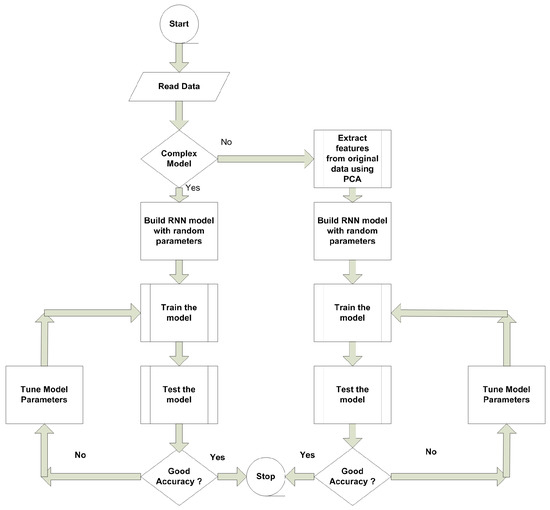
Figure 2.
Proposed work flow diagram.
3. Result Analysis
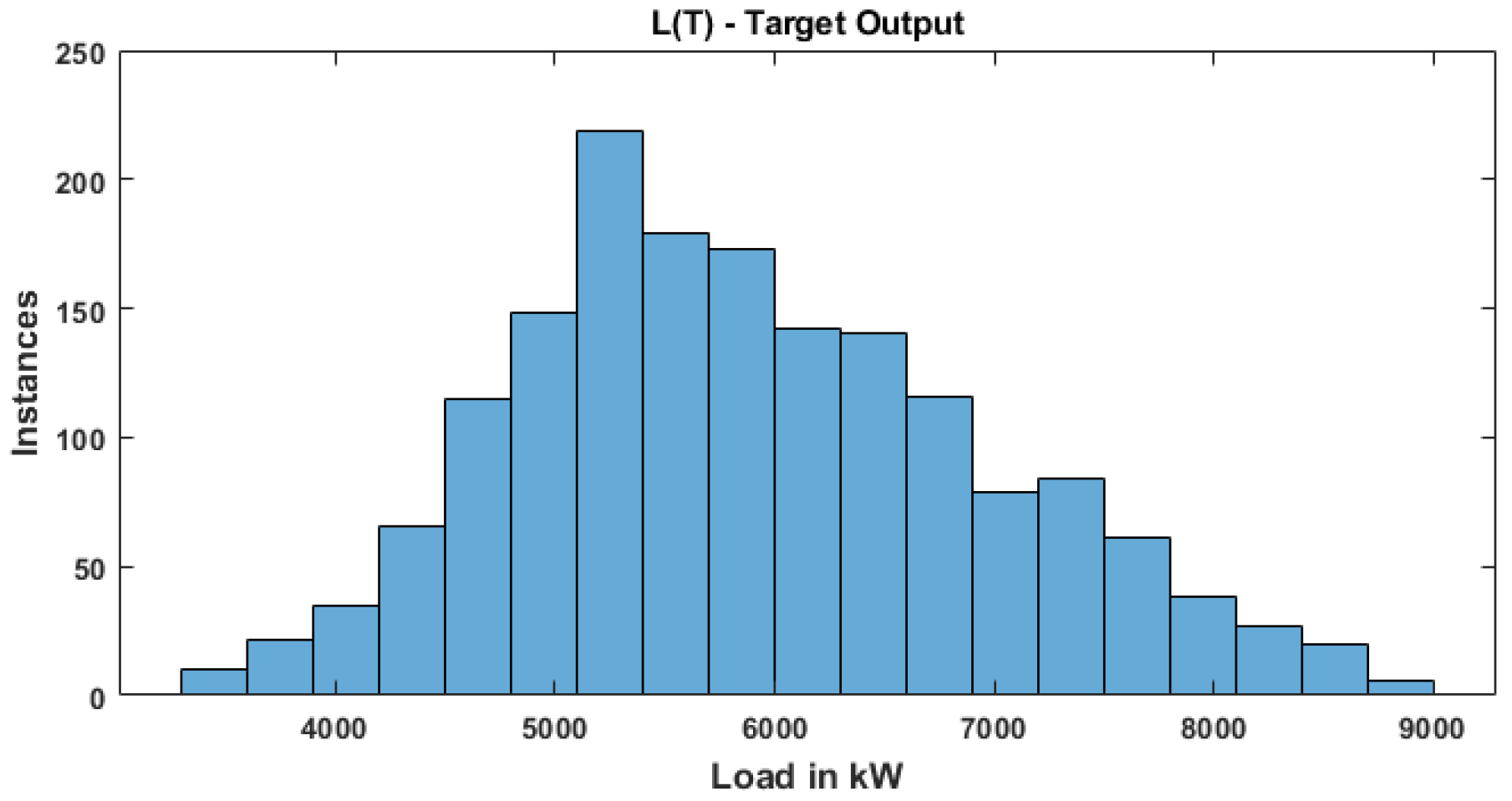
Data was captured from [28] to train and test the models. This load data consists of a total of 2184 samples (91 days × 24 h) and these data are rearranged into a 1680, i.e., matrix. The first nine columns represent nine input features, whereas the 10th column represents target output (load). Statistical features of the load dataset that have been used to train the RNN model is presented in Table 3. The frequency distribution of output load data values is represented in terms of histogram plot as shown in Figure 3,

Table 3.
Load data statistics.

Figure 3.
Histogram plot for output feature .
3.1. Load Forecasting for HAM-(RHM-1)
The train and test datasets for “RHM-1” comprise a total of 1680 observations. Out of 1680 load data samples, 1512 were chosen for training and 168 for validation. For several hidden neurons the performance of the model in terms of performance metrics was observed during both training and testing, as shown in Table 4. Table 4 indicates that models performance in terms of training and test accuracy grows to 13 hidden neurons. If the number of occluded neurons exceeds 13 it is excessively fit and leads in further test errors. At this point, the “RHM-1” is deemed an optimum model, with 13 hidden neurons.

Table 4.
Impact of hidden neurons on the performance of the model “RHM-1”.
In addition, the number of hidden layers in the RNN model was raised to boost the model’s performance (RHM-1). The performance of the model with different levels was measured using the performance metrics as illustrated in Table 5. Each hidden layer consists of 13 neurons. It was seen from Table 5 that the model performs well with only one hidden layer. The test error values rise for the same loss of training if the number of hidden layers is more than one. This indicates that if the number of hidden layers is greater than one, then the model gets overfit. Furthermore, as the number of hidden layers rises, the number of training parameters increases the needed memory and processing time.

Table 5.
Impact of hidden layers on the performance of the model “RHM-1”.
The suggested model, i.e., RNN-HAM-Mode11, has been trained 10 fold in the same data set and is judged to be the ideal load prediction model in real time when the best values for training and validation errors were given. The performance of the suggested ‘RHM-1’ model is observed in stochastic environment and shown in Table 6. For all error matrices that reflect the sturdy behavior of the “RHM-1” architecture, the standard deviation is noted to be virtually null.

Table 6.
Statistical performance of the model (RHM-1).
3.2. Load Forecasting for HAM-(RHM-2)
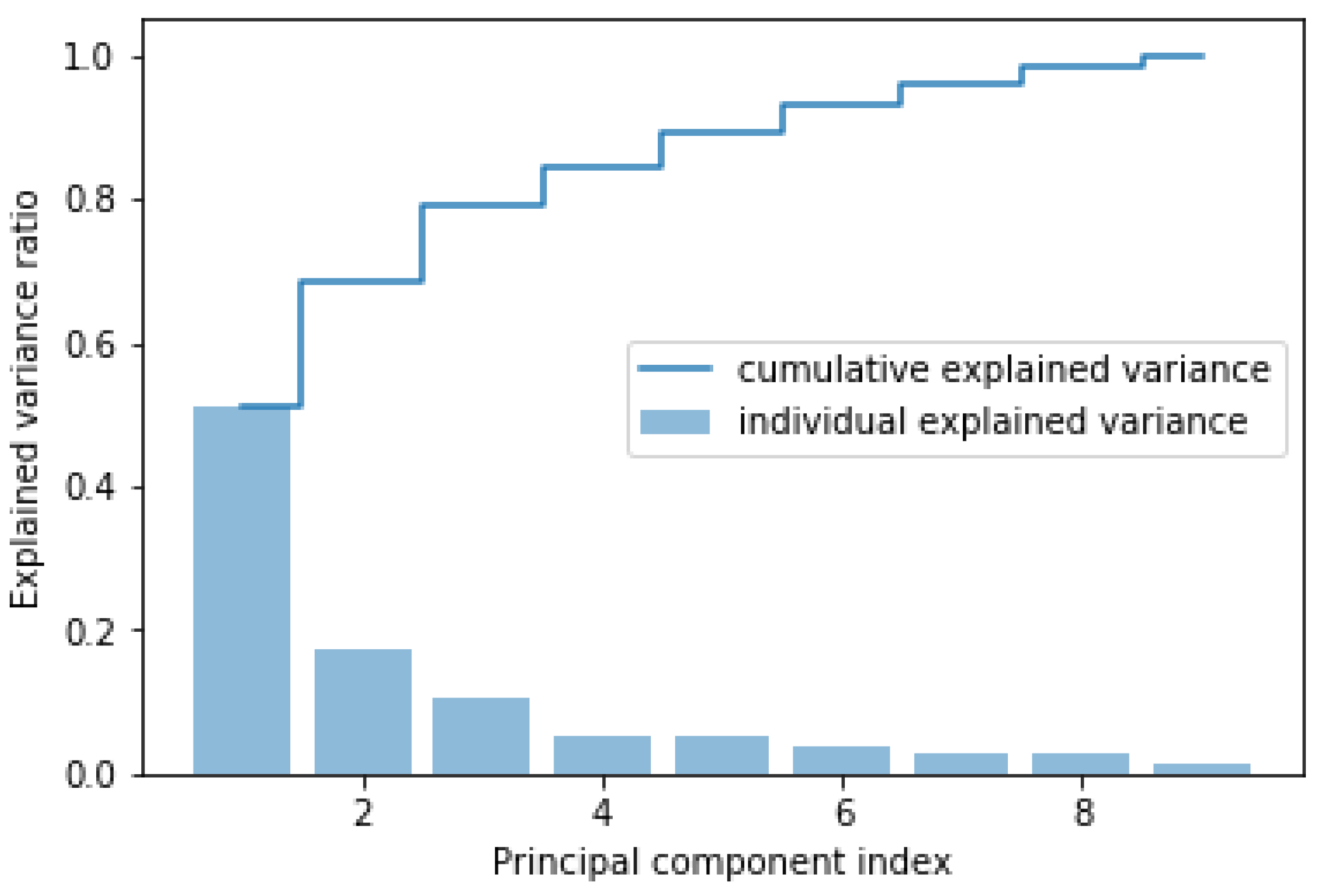
The PCA algorithm is applied to the input features of the load dataset to find the principal components. The total variance in the dataset covered by each principal component and the cumulative variance covered are shown in Figure 4. It shows that six principal components cover almost 90% of the variance in the load dataset. Outcome of PCA that feeda as input to RNN for first 10 datasamples are presented in Table 7.
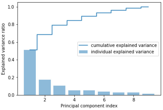
Figure 4.
Variance in the load dataset (for HAM) covered by principal components.

Table 7.
Pricipal components for first 10 load data samples used for HAM.
The suggested “RNN-HAM-Model2” has been trained and tested with different number of hidden neurons to detect the optimal “RNN-HAM-Model2”. The model is observed in terms of performance measures in the form of Table 8 throughout both the training and testing. The performance of the model has been growing up to 11 hidden neurons with regard to training and test accuracy, the Table 8 was found. So the optimum model is at this point in “RHM-2” with 11 hidden neurons.

Table 8.
Impact of hidden neurons on the performance of the model “RHM-2”.
The number of layers covered by this model (RHM-2), which was meant to predict loading one hour sooner, has also been increased. Each layer is comprised of 11 neurons and performance measurement metrics as shown in Table 9 of a model with different layers were observed. In Table 9, good test performance was found with only one hidden layer. If the number of layers concealed is more than one, then the numbers for the test error rise, then it is overfit if the number of layers hidden is higher than the one.

Table 9.
Impact of hidden layers on the performance of the model “RHM-2”.
The model, i.e., RNN-HAM-Model 2, is trained ten times in an identical data set and is regarded to be the ideal model for real-time load prediction for training and validation errors. Table 10 presents the performance of the suggested model, that is, ‘RHM-2’ inside stochastic environments, and it is shown that for all error matrices, which indicate strong performance of the RHM-2 architecture, a standard deviation of practically zero is present.

Table 10.
Observations of performance of the RHM-2 in stochastic environment.
In Table 11, An original model, i.e., the RHM-1, is compared with the compressed model, i.e., RHM-2. The RHM-2 is tiny with 210 parameters in relation to the 313 RHM-1. Due to the little dimensional compression of the model, RHM-2 losses compared to RHM-1 are somewhat greater. Although the workout parameters of “RHM-2” were compressed in 32.91%, losses of MSE, RMSE and MAE correspondingly rose by 4.5%, 1.7% and 5%.

Table 11.
Comparison between RNN models for HAM.
3.3. Load Forecasting for DAM-(RDM-1)
The suggested model is conditioned and assessed using different numbers of hidden neurons in order to identify the best RDM-1. In terms of the performance metrics provided in Table 12, the model performance during training and testing is noted. The outputs of a model have been seen in Table 12 as regards training and test accuracy increases up to 13 hidden neurons. RDM-1 is deemed an optimum model at this moment with 13 hidden neurons.

Table 12.
Impact of hidden neurons on the performance of the model “RDM-1”.
In order to enhance performance (RDM-1), the numbers of hidden layers in the RNN models are increased. There are 13 neurons per hidden layer, the performance of which is demonstrated in Table 13 is illustrated by performance metrics for the model with different layers. The model with only one hidden layer has been noticeable in Table 13 for a positive test performance.

Table 13.
Impact of hidden layers on the performance of the model “RDM-1”.
The model recommended, i.e., RDM-1 was trained on the same dataset 10 times and is regarded the best way to forecast loads in real time in terms of training and validation errors. Statistical analyses of the training behaviour, shown in Table 14, indicate that the standard deviation in the RDM-1 Architecture is practically zero for all error matrices described as robust behaviour.

Table 14.
Statistical training performance of model RDM-1.
3.4. Load Forecasting for DAM-(RDM-2)
The PCA algorithm is applied to the input features of the load dataset to find the principal components. Load dataset consists of a total of 6 input features, i.e., , , , , and , and one output . The total variance in the dataset covered by each principal component and the cumulative variance covered are shown in Figure 5. Figure 5 shows that four principal components cover almost 90% of the variance in the load dataset. Thus, six input features, i.e., , , , , and for each dataset sample, are translated into four principal components. These four principal components were used to train the RDM-2. RDM-2 was therefore equipped with four input neurons and one output neuron.

Figure 5.
Variance in the load dataset (for DAM) covered by principal components.
In order to find the optimal “RDM-2” in terms of the number of hidden neurons, the proposed “RDM-2” is equipped and evaluated with different numbers of hidden neurons. The performance of the model during both training and testing is observed in terms of performance metrics as shown in Table 15. From Table 15, it has been observed that the performance of the model has increased to 7 hidden neurons in terms of training and test accuracy. At this point, therefore, RDM-2 with 7 hidden neurons is considered to be an optimal model.

Table 15.
Impact of hidden neurons on the performance of the model “RDM-2”.
In addition, there have been higher numbers of hidden layers to improve the model’s efficiency (RDM-2) for load prediction. Each hidden layer has 7 neurons and performance metrics as given in Table 15 demonstrate the output of the model with different layers. From Table 16, good test performance with just one hidden layer has been noticed. If the number is more than one, the values for the test error are increased, the model becomes over-fit if the number of hidden layers is higher than one.

Table 16.
Impact of hidden layers on the performance of the model “RDM-2”.
The recommended model, i.e., RDM-2, is trained ten times on the same data set and is deemed an ideal model for forecasting the load in real time when it has given the best values in relation to training and validation errors. In Table 17 the statistical analysis of the suggested model workouts reveals that the standard deviation is practically Nil for all the error matrices defining resilient behaviour in the RDM-2 architecture.

Table 17.
Statistical analysis of RDM-2 architecture.
In Table 18, the comparison is shown to the original model, namely the RDM-1, and the compressed model. In comparison with the RDM-1 with 274 parameters the size of RDM-2 is modest with 92 parameters. The model RDM-2 exhibited somewhat higher test losses than the model RDM-1, due to the distortion of the model with the lower dimensionality. Although the training size of “RDM-2” has been reduced by 66.42%, losses, i.e, MSE, RMSE and MAE correspondingly have risen by 2.5%, 0.7% and 1.9%.

Table 18.
Comparison between RNN models for Day Ahead Markets (DAM).
3.5. Comparative Result Analysis
The performance of the proposed RNN model was verified by comparing with ANN models [22,29,30], Regression models [19] and LSTM model [20] as presented in Table 19. It can be observed that the RNN model was able to predict the load with good accuracy. The performance of the model was compared statistically with models proposed in [22,29,30] and statistical metrics presented in Table 20, showing that the proposed RNN model is statistically robust with zero standard deviation.

Table 19.
Validation of models in testing environment.

Table 20.
Validation in probabilistic environment.
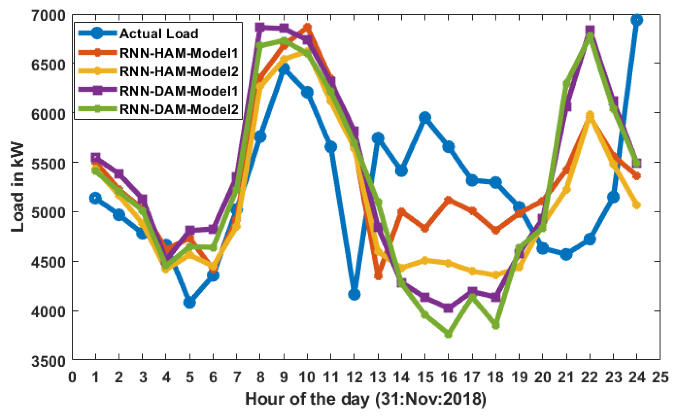
The comparison with real load on 30 November 2018 of the loads forecast is shown in Figure 6 utilising several suggested RNN models for hourly and day ahead markets. The expected load of RHM-1 and RHM-2 is closer to real load than RDM-1 and RDM-2, since the former model forecast loads an hour earlier and one day in advance.

Figure 6.
Actual load vs. predicted load.
In Table 21, the total training time for various RNN systems with varying batch sizes is reported. As clearly shown, if we refer to batch size 32 (last row) the number of back-propagation is significantly reduced with respect to batch size 1, thus resulting in a lower computational effort as wanted by the authors’ initial design.

Table 21.
Training computation time (s).
In order to show the advantages of using a non-linear approach, the performance of the proposed RNN model was verified by comparing with commonly used linear models like Auto Regression (AR) [31], Moving Average (MA) [32], Auto-regressive Moving Average (ARMA) [33], Auto-regressive Integrated Moving Average (ARIMA) [34] and Simple Exponential Smoothing (SES) [35], as presented in Table 22. It can be observed that the RNN model was able to perform better than traditional linear methods in terms of both RMSE and MAE values of predicted load. Although some concerns have been reported in literature with respect to using MAE as an accuracy indicator [36], we preferred to show both RMSE and MAE error metrics for the sake of comparison with results in previously cited references.

Table 22.
Validation of models in testing environment by comparing with classical models.
4. Conclusions
An accurate short-term projection of the electric load allows utilities to efficiently sell their electricity and manage the system on more steady, trustworthy expected information.
In order to ensure that utilities can efficiently trade in energy, the authors proposed different RNN models, notably RHM-1 and RDM-1 for predicting the load accurately. Lightweight models, i.e., RHM-2 and RDM-2, present reduced input features by means of PCA. These light weight models predicted the load with nearly the almost near accuracy as the original ones but reducing the complexity of the model a lot comparing to original models.
In this paper, real time load data were obtained from a 33/11 kV substation near the Kakatiya University in Warangal (India) for training and testing different RNN models in a practical case study. In order to identify outliers and also to observe the skewedness of data, suitable preprocessing techniques were employed.
The suggested RNN models were verified in terms of error measures by correlating them to those reported in the literature. Randomness in forecast using suggested RNN models is noticed and compared to current models.
Future works could additional take into account external factors and habits, e.g., climate, weather conditions and particular human behavioral patterns.
Author Contributions
V.V. constructed the research theories and methods, developed the basic idea of the study, performed the computer simulation and analyses; V.V., F.G. and M.M. conducted the preliminary research; D.R.C., F.G. and M.M. worked on proof read of this article; V.V., F.G. and M.M. worked on document preparation; V.V. served as the head researcher in charge of the overall content of this study as well as modifications made. All authors have read and agreed to the published version of the manuscript.
Funding
This research activity was partly supported by the EU Horizon 2020 project PLATOON (Grant agreement ID: 872592) https://platoon-project.eu/ (accessed on 17 January 2022).
Institutional Review Board Statement
Not applicable.
Informed Consent Statement
Not applicable.
Data Availability Statement
The datasets generated during and/or analysed during the current study are available in the Mendeley Data repository, https://data.mendeley.com/datasets/ycfwwyyx7d/2 (accessed on 17 January 2022).
Acknowledgments
We thank S R Engineering College Warangal, Telangana State, India and POLITECNICO DI MILANO, Italy for supporting us during this work. We also thank engineers in 33/11 kV substation near Kakatiya University in Warangal for providing the historical load data.
Conflicts of Interest
The authors declare that they have no conflict of interest.
Abbreviations
The following abbreviations are used in this manuscript:
| Load at hour | |
| Load at one hour before from the time of prediction | |
| Load at two hours before from the time of prediction | |
| Load at three hours before from time of prediction | |
| Load at one day before from the time of prediction | |
| Load at two days before from the time of prediction | |
| Load at three days before from time of prediction | |
| Load at one week before from the time of prediction | |
| Load at two weeks before from the time of prediction | |
| Load at three weeks before from time of prediction | |
| MSE | Mean Square Error |
| MAE | Mean Absolute Error |
| RMSE | Root Mean Square Error |
| a | Hidden neuron current activation state |
| a | Hidden neuron previous activation state |
| Bias parameter for hidden layer | |
| Bias parameter for output layer | |
| Weight matrix between input and hidden layer | |
| Weight matrix between output and hidden layer | |
| DAM | Day ahead market |
| HAM | Hourly ahead market |
| RHM-1 | Recurrent Neural Network Model for Hourly Ahead Market |
| RHM-2 | Light weight recurrent neural network Model for Hourly Ahead Market |
| RDM-1 | Recurrent Neural Network Model for day ahead market |
| RDM-2 | Light weight recurrent neural network Model for day ahead market |
| Actual load from sample | |
| Predicted load with sample |
References
- Ahmad, T.; Chen, H. A review on machine learning forecasting growth trends and their real-time applications in different energy systems. Sustain. Cities Soc. 2020, 54, 102010. [Google Scholar] [CrossRef]
- Akhavan-Hejazi, H.; Mohsenian-Rad, H. Power systems big data analytics: An assessment of paradigm shift barriers and prospects. Energy Rep. 2018, 4, 91–100. [Google Scholar] [CrossRef]
- Almeshaiei, E.; Soltan, H. A methodology for electric power load forecasting. Alex. Eng. J. 2011, 50, 137–144. [Google Scholar] [CrossRef] [Green Version]
- Khodayar, M.E.; Wu, H. Demand forecasting in the Smart Grid paradigm: Features and challenges. Electr. J. 2015, 28, 51–62. [Google Scholar] [CrossRef]
- Mansoor, M.; Grimaccia, F.; Leva, S.; Mussetta, M. Comparison of echo state network and feed-forward neural networks in electrical load forecasting for demand response programs. Math. Comput. Simul. 2021, 184, 282–293. [Google Scholar] [CrossRef]
- Su, P.; Tian, X.; Wang, Y.; Deng, S.; Zhao, J.; An, Q.; Wang, Y. Recent trends in load forecasting technology for the operation optimization of distributed energy system. Energies 2017, 10, 1303. [Google Scholar] [CrossRef] [Green Version]
- Zheng, X.; Ran, X.; Cai, M. Short-term load forecasting of power system based on neural network intelligent algorithm. IEEE Access 2020. [Google Scholar] [CrossRef]
- Vasudevan, S. One-Step-Ahead Load Forecasting for Smart Grid Applications. Ph.D. Thesis, The Ohio State University, Columbus, OH, USA, 2011. [Google Scholar]
- Neusser, L.; Canha, L.N. Real-time load forecasting for demand side management with only a few days of history available. In Proceedings of the 4th International Conference on Power Engineering, Energy and Electrical Drives, Istanbul, Turkey, 13–17 May 2013; pp. 911–914. [Google Scholar]
- Singh, A.K.; Khatoon, S.; Muazzam, M.; Chaturvedi, D.K. Load forecasting techniques and methodologies: A review. In Proceedings of the 2012 2nd International Conference on Power, Control and Embedded Systems, Allahabad, India, 17–19 December 2012; pp. 1–10.
- Ahmad, F.; Alam, M.S. Assessment of power exchange based electricity market in India. Energy Strategy Rev. 2019, 23, 163–177. [Google Scholar] [CrossRef]
- Massaoudi, M.; Refaat, S.S.; Chihi, I.; Trabelsi, M.; Oueslati, F.S.; Abu-Rub, H. A novel stacked generalization ensemble-based hybrid LGBM-XGB-MLP model for Short-Term Load Forecasting. Energy 2021, 214, 118874. [Google Scholar] [CrossRef]
- Yin, L.; Xie, J. Multi-temporal-spatial-scale temporal convolution network for short-term load forecasting of power systems. Appl. Energy 2021, 283, 116328. [Google Scholar] [CrossRef]
- Syed, D.; Abu-Rub, H.; Ghrayeb, A.; Refaat, S.S.; Houchati, M.; Bouhali, O.; Bañales, S. Deep learning-based short-term load forecasting approach in smart grid with clustering and consumption pattern recognition. IEEE Access 2021, 9, 54992–55008. [Google Scholar] [CrossRef]
- Munkhammar, J.; van der Meer, D.; Widén, J. Very short term load forecasting of residential electricity consumption using the Markov-chain mixture distribution (MCM) model. Appl. Energy 2021, 282, 116180. [Google Scholar] [CrossRef]
- Guo, W.; Che, L.; Shahidehpour, M.; Wan, X. Machine-Learning based methods in short-term load forecasting. Electr. J. 2021, 34, 106884. [Google Scholar] [CrossRef]
- Eskandari, H.; Imani, M.; Moghaddam, M.P. Convolutional and recurrent neural network based model for short-term load forecasting. Electr. Power Syst. Res. 2021, 195, 107173. [Google Scholar] [CrossRef]
- Sheng, Z.; Wang, H.; Chen, G.; Zhou, B.; Sun, J. Convolutional residual network to short-term load forecasting. Appl. Intell. 2021, 51, 2485–2499. [Google Scholar] [CrossRef]
- Veeramsetty, V.; Mohnot, A.; Singal, G.; Salkuti, S.R. Short Term Active Power Load Prediction on A 33/11 kV Substation Using Regression Models. Energies 2021, 14, 2981. [Google Scholar] [CrossRef]
- Veeramsetty, V.; Chandra, D.R.; Salkuti, S.R. Short-term electric power load forecasting using factor analysis and long short-term memory for smart cities. Int. J. Circuit Theory Appl. 2021, 49, 1678–1703. [Google Scholar] [CrossRef]
- Grimaccia, F.; Mussetta, M.; Zich, R. Neuro-fuzzy predictive model for PV energy production based on weather forecast. In Proceedings of the 2011 IEEE International Conference on Fuzzy Systems (FUZZ-IEEE 2011), Taipei, Taiwan, 27–30 June 2011; pp. 2454–2457. [Google Scholar] [CrossRef]
- Veeramsetty, V.; Deshmukh, R. Electric power load forecasting on a 33/11 kV substation using artificial neural networks. SN Appl. Sci. 2020, 2, 855. [Google Scholar] [CrossRef] [Green Version]
- Hong, T.; Pinson, P.; Fan, S.; Zareipour, H.; Troccoli, A.; Hyndman, R.J. Probabilistic energy forecasting: Global Energy Forecasting Competition 2014 and beyond. Int. J. Forecast. 2016, 32, 896–913. [Google Scholar] [CrossRef] [Green Version]
- Veeramsetty, V.; Reddy, K.R.; Santhosh, M.; Mohnot, A.; Singal, G. Short-term electric power load forecasting using random forest and gated recurrent unit. Electr. Eng. 2021, 1–23. [Google Scholar] [CrossRef]
- Abdi, H.; Williams, L.J. Principal component analysis. Wiley Interdiscip. Rev. Comput. Stat. 2010, 2, 433–459. [Google Scholar] [CrossRef]
- Mandic, D.P.; Chambers, J. Recurrent Neural Networks for Prediction: Learning Algorithms, Architectures and Stability; John Wiley & Sons, Inc.: Hoboken, NJ, USA, 2001. [Google Scholar]
- Karri, C.; Durgam, R.; Raghuram, K. Electricity Price Forecasting in Deregulated Power Markets using Wavelet-ANFIS-KHA. In Proceedings of the 2018 International Conference on Computing, Power and Communication Technologies (GUCON), Greater Noida, India, 28–29 September 2018; pp. 982–987. [Google Scholar]
- Veeramsetty, V. Active Power Load Dataset. 2020. Available online: https://data.mendeley.com/datasets/ycfwwyyx7d/2 (accessed on 13 December 2021).
- Shaloudegi, K.; Madinehi, N.; Hosseinian, S.; Abyaneh, H.A. A novel policy for locational marginal price calculation in distribution systems based on loss reduction allocation using game theory. IEEE Trans. Power Syst. 2012, 27, 811–820. [Google Scholar] [CrossRef]
- Veeramsetty, V.; Chintham, V.; Vinod Kumar, D. Proportional nucleolus game theory–based locational marginal price computation for loss and emission reduction in a radial distribution system. Int. Trans. Electr. Energy Syst. 2018, 28, e2573. [Google Scholar] [CrossRef]
- Hannan, E.J.; Kavalieris, L. Regression, autoregression models. J. Time Ser. Anal. 1986, 7, 27–49. [Google Scholar] [CrossRef]
- Johnston, F.; Boyland, J.; Meadows, M.; Shale, E. Some properties of a simple moving average when applied to forecasting a time series. J. Oper. Res. Soc. 1999, 50, 1267–1271. [Google Scholar] [CrossRef]
- Chen, J.F.; Wang, W.M.; Huang, C.M. Analysis of an adaptive time-series autoregressive moving-average (ARMA) model for short-term load forecasting. Electr. Power Syst. Res. 1995, 34, 187–196. [Google Scholar] [CrossRef]
- Contreras, J.; Espinola, R.; Nogales, F.J.; Conejo, A.J. ARIMA models to predict next-day electricity prices. IEEE Trans. Power Syst. 2003, 18, 1014–1020. [Google Scholar] [CrossRef]
- Haben, S.; Giasemidis, G.; Ziel, F.; Arora, S. Short term load forecasting and the effect of temperature at the low voltage level. Int. J. Forecast. 2019, 35, 1469–1484. [Google Scholar] [CrossRef] [Green Version]
- Gneiting, T. Making and Evaluating Point Forecasts. J. Am. Stat. Assoc. 2011, 106, 746–762. [Google Scholar] [CrossRef] [Green Version]
Publisher’s Note: MDPI stays neutral with regard to jurisdictional claims in published maps and institutional affiliations. |
© 2022 by the authors. Licensee MDPI, Basel, Switzerland. This article is an open access article distributed under the terms and conditions of the Creative Commons Attribution (CC BY) license (https://creativecommons.org/licenses/by/4.0/).

