Abstract
This work proposes and evaluates a method for the nowcasting of solar irradiance variability in multiple time horizons, namely 5, 10, and 15 min ahead. The method is based on a Convolutional Neural Network structure that exploits infrared sky images acquired through an All-Sky Imager to estimate the range of possible values that the Clear-Sky Index will possibly assume over a selected forecast horizon. All data available, from the infrared images to the measurements of Global Horizontal Irradiance (necessary in order to compute Clear-Sky Index), are acquired at SolarTechLAB in Politecnico di Milano. The proposed method demonstrated a discrete performance level, with an accuracy peak for the 5 min time horizon, where about 65% of the available samples are attributed to the correct range of Clear-Sky Index values.
1. Introduction
Power generation from a renewable energy source (RES) is becoming increasingly popular to meet the ever-growing global energy demand and to limit fossil fuel-related greenhouse gas emissions. In detail, over the last few decades, solar and wind have experienced significant growth in terms of installed capacity together with continuous technological improvement [1].
Regarding solar energy and, more specifically, photovoltaic (PV) technology, its rapid growth has faced multiple technical obstacles, such as low solar cell efficiency, and economic problems, such as high cost of materials [2]. Theoretical analyses show that solar energy alone, with adequate technology to collect and store it, could meet the energy demand of the entire world [3]. For example, global energy consumption recorded in 2017 was around 18.1 TW and is projected to be around 28 TW by 2050, while land-based solar energy in one year is estimated at 23,000 TW. Furthermore, solar energy is a renewable source, and its exploitation for energy production does not cause polluting emissions and greenhouse gases [4].
The energy produced by a RES is characterized by fluctuations, which are dependent on various environmental and meteorological parameters. Hence, a high penetration of this type of source into the electrical system is challenging [5]. In a scenario where renewable energies play a fundamental role in the energy supply, a reliable forecast of energy production is essential to properly manage the electrical system [6]. For this reason, RES energy production forecasting is one of the most popular topics within the scientific community today [7]. Solar energy forecasting is useful for regulating the routine operation of electrical grids and microgrids with integrated solar power generation [8,9], enabling imbalances in energy production and consumption to be minimized [10]. Furthermore, it is a fundamental tool during the identification of the potential location for the photovoltaic installation and the subsequent planning phase [11].
Different forecasting horizons can be identified. They are highly dependent on the forecasting target. In particular, for power production, two different classifications can be identified: the first one is related to the operation and maintenance of the grid, while the second one is closely related to electricity market definitions [12,13]. By analyzing [14], it is possible to identify three main horizons: the long-term forecasting, corresponding to the day-ahead forecast, the mid-term from 1 day down to 6 h, the short-term from 6 h to 30 min, and nowcasting, which includes the forecast horizons under 30 min. The nowcasting time horizon, the central topic of the present work, is crucial in solving grid stability issues and optimizing the microgrid’s energy management systems [15]. Moreover, it is vital in regulating the electricity market whenever a solar power production facility is connected to the electrical grid [16]. In nowcasting, the object of the solar forecast is the solar irradiance, which directly influences the power produced by PV modules.
Nowcasting methods can be roughly classified into physical and data-driven models [17]. Three main types of solar radiation forecasting methods are considered in the scientific literature: numerical weather forecasting (NWP) models, appropriate for long-term forecasting; satellite techniques, appropriate for time horizons up to 8 h ahead; ground techniques, appropriate for nowcasting. NWP models are based on a set of differential equations that describe the physical phenomena of interest. In order to achieve an accurate forecast, they require a proper definition of initial conditions [18]. Furthermore, images captured from a satellite are useful for forecasting tasks, providing an overview of large-scale weather systems and their movement. Ground-based techniques exploit All-Sky Imagers (ASIs), cameras capable of acquiring pictures of the sky through an hemispherical mirror, which are helpful in estimating cloudiness [19]. The ASI can be configured for different operational environments and network designs, from a standalone edge computing model to a fully integrated node in a distributed, cloud-computing-based microgrid [20].
The most challenging part of nowcasting is the analysis of transient clouds and hence the estimation of type, cover, and movement [21]. These challenges are addressed by computer vision [22], a branch of computer science dedicated to the emulation of human visual system capabilities that allows computers to recognize elements in pictures and videos in the same manner as people. In recent years, thanks to the development of artificial intelligence and deep learning, this field took great leaps forward that enabled the ability to perform several tasks that previously could not be accomplished without artificially complex methods [23]. A deep-learning tool that achieved excellent results in several works from scientific literature is the Convolutional Neural Network (CNN) [24]. In computer vision tasks, CNNs have several advantages over traditional Neural Networks because they are specifically optimized in extracting and learning features from images [17].
The aim of this work is to exploit full-sky infrared images to predict, by means of a CNN, the Clear-Sky Index (CSI) in different time horizons, namely 5, 10, and 15 min. In this work, all available images are acquired by an ASI installed at the SolarTechLAB in Politecnico di Milano. Images are acquired in RGB format once per minute: this sampling rate is limited by the available hardware. In order to reduce the dataset required for the training of convolutionary neural networks, here, it was, therefore, decided to crop the images in the portion around the sun. This helps the applicability of the method because in many cases it is not possible to have a sufficiently large dataset.
2. Solar Irradiance Forecasting Procedure
In this section, all the steps of the procedure adopted to perform the forecast of solar irradiation are discussed, from preprocessing the dataset to the development of the deep-learning model. This section is structured as follows: Section 2.1 and Section 2.2 describe the available data and the preprocessing stages, and Section 2.3 describes the structure of the adopted CNN.
Available data consist of infrared sky images captured by specific ASIs and Global Horizontal Irradiation (GHI) measurements. In detail, they are acquired for all the days comprised between September 2019 and April 2020, with a one-minute time step and considering only the daylight hours.
2.1. Image Processing Techniques
The available images undergo a specific pre-processing procedure with two objectives. The first is to obtain a format suitable for processing with a CNN template. The second goal is to be able to reduce the number of samples required for CNN training.
The instrumentation in SolarTechLAB is capable of acquiring sky images with a multi-spectral approach. Figure 1, for instance, reports an example of a same sky view acquired by two different sensors in optical and infrared spectral regions, respectively. However, only the infrared images are included in the dataset exploited in the present work since they are less prone to saturation issues and allow effectively identifying the sun position.
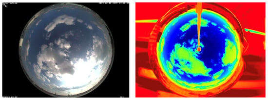
Figure 1.
Same sky view acquired through different sensors in optical and infrared spectral regions.
From previous studies, it appears that the most significant areas for nowcasting are those around the sun. In fact, these areas are the ones responsible for direct radiation. Starting from this consideration, in the available infrared images, a square region surrounding the position of the sun is cropped, as shown in Figure 2. This operation allows reducing the computational burden of the training phase, both for the number of images required and the computational time.
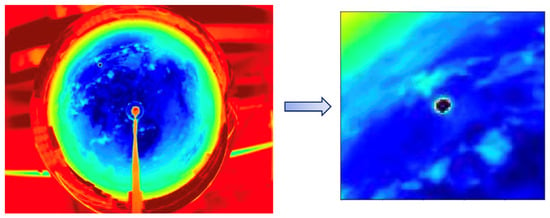
Figure 2.
The infrared images are cropped based on the sun’s position in a way that the sun is located in the middle of each image in a square shape. The images are cropped since only the area around sun is relevant.
The available infrared images undergo specific preprocessing that aims to isolate the region surrounding the sun’s location and a cleaning procedure that aims to exclude rainy conditions from the data involved in the CNN development, and then the forecast model is tested.
2.2. Classification Phase
Once the images are properly treated, they are classified according to two different criteria. The first criterion aims at dividing the images according to the presence of precipitation. Specifically, two different groups of images can be identified, representing, respectively:
- Dry conditions: clear sky conditions, characterized by the absence of significant cloud coverage, and covered sky conditions, characterized by the presence of significant cloud coverage without precipitation, are considered together as a single group.
- Rainy conditions, characterized by significant cloud coverage and the presence of water droplets on the hemispherical mirror surfaces of ASIs.
In Figure 3, examples of clear sky (a), covered sky (b), and rainy (c) conditions are reported.
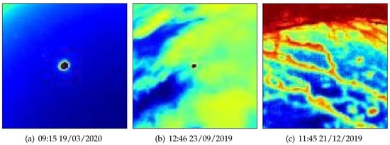
Figure 3.
Examples images from each of the three defined groups: (a) dry conditions—clear sky; (b) dry conditions—covered sky; (c) rainy conditions.
Images related to rainy conditions are identified thanks to a rain gauge installed in the weather station of the SolarTechLAB and are removed from the dataset involved in the solar irradiance forecast.
The second classification criterion consists of dividing the images into five different groups on the basis of the Clear-Sky Index value, defined as [25,26]:
In the equation, is the the measured Global Horizontal Irradiation, while is the Global Horizontal Irradiation in clear sky conditions. In other words, CSI corresponds to a normalized GHI, which allows removing the effects of seasonal changes from the GHI itself [27].
In more detail, images are grouped into five distinct classes based on strict threshold values of CSI, as reported in Table 1. “Over-irradiance” is a particular condition where solar radiation multiple reflections between the ground and direct beam could result in greater solar radiation levels on the pyranometer with respect to Clear Sky conditions.Hence, the CSI, which is the ratio of measured irradiance at ground level to the estimated irradiance in clear sky conditions at ground level, could go beyond 1, as shown in [28].

Table 1.
Threshold values of CSI for classes definition.
Figure 4 depicts the overall double-step classification scheme that allows preprocessing the data.
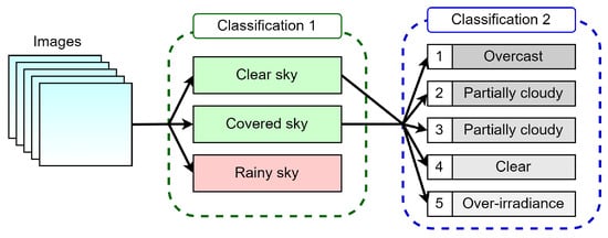
Figure 4.
Double-step classification scheme.
2.3. Model Development
In the present work, a deep-learning model for image classification, namely a CNN, is developed. The idea of CNNs is derived from studies on the brain’s visual cortex. Each of the neurons dedicated to vision processes information derived from a limited region of the visual field only. Moreover, the receptive fields of different neurons may overlap, and, all together, they cover the entire visual field. This structure, capable of detecting complex patterns in any region of the visual field, inspired the researcher to develop a Neural Network architecture that gradually evolved into the current CNN [29].
In further detail, the typical CNN structure is capable of learning features from input images through a sequence of convolutional and pooling layers [30]. The convolutional layer is the crucial building block of CNNs: neurons in this type of layer are not connected to every pixel in the input image, only to pixels in their corresponding receptive fields. The weight of a neuron is represented by a filter (or convolution kernel) that, when applied to the image, is able to extract features from it. During the training phase, the convolutional layer learns which is the best-suited convolution kernel to fulfill a specific task [31]. On the other hand, the pooling layer has the goal of subsampling the input image in order to reduce the computational load, the memory usage, and the number of network parameters to be tuned. As in convolutional layers, each neuron is connected to a restricted region of the previous layer. Moreover, neurons in this layer do not have weights: all they do is aggregate the inputs according to a specific aggregation function, such as “max” or “mean”. After being processed in the cascade of convolutional and pooling layers, the information flow is flattened, i.e., it is structured in a suitable format to be further processed.
After the feature learning step, the flowing information is flattened (properly structured in order to be further processed) and delivered to a fully connected layer that performs the classification step.
The structure of the CNN adopted in the present work is presented in Figure 5. Hidden patterns are extracted from images by means of two couples of convolutional and pooling layers. Then, a flattening layer and a fully connected layer perform the feature-based classification. Each convolutional layer adopts 30 convolution kernels with a 4 × 4 squared shape and a stride equal to 1, while each pooling layer exploits pooling kernels with a 4 × 4 squared shape and a stride equal to 4. The number of kernels, their shape, and the number of neurons in the fully connected layer are chosen through a sensitivity analysis procedure that allows selecting a proper configuration capable of achieving reasonable performance.

Figure 5.
Architecture of the adopted CNN model.
Concerning the available infrared images, 70% are exploited as the training set, while another 15% constitutes the validation set. The remaining 15% of data is used as the test set.
3. Results and Discussion
In this section, the forecasting performance achieved with the proposed method is reported considering all three different forecasting horizons considered, i.e., 5, 10 and 15 min, respectively.
Firstly, the instrumentation used in this case study is described, then the numerical results are presented.
3.1. Case Study
Weather parameters are monitored at the SolarTechLAB with a meteorological station equipped with a solar irradiance sensor, temperature and humidity sensors, a wind speed and direction sensor, and a rain collector. Solar irradiance is measured with two secondary standard pyranometers for the measurement of the total irradiance on horizontal and 30° tilt planes. In addition, a pyranometer with a shadow band is available for measuring the diffuse irradiance.
The main characteristics of the sensors, together with the temperature measuring equipment, are described in Table 2.

Table 2.
Detailed characeristics of weather station.
The meteorological station performs ambient conditions measurements every ten seconds. The average, maximum, minimum, and standard deviation of the values measured by the sensors are calculated every minute, and these values are stored in a database.
The SkyCam system comprises a long-wavelength infrared camera placed over a hemispherical mirror reflecting the sky. It thus provides full-sky coverage, equivalent to a 180° × 360° field-of-view. The SkyCam uses a curved mirror with a diameter of 35 cm, coated with chrome. It is designed to be dust-tight, to resist liquid ingress, and to operate in the −20 to +60 °C ambient temperature range. The resolution of the raw images is 640 × 480 pixels. The sky-imager possesses its own mechanical-optical arrangement and orientation once deployed. A geometrical calibration is therefore performed at each site to retrieve the optical intrinsic parameters of the sky-imager. The calibration process is fully automated and uses an automatic algorithm based on the solar position captured during clear-sky days over full sun paths to calibrate the pixels. In addition to the geometric calibration, automated detection of the mask is performed to distinguish between useful pixels and useless pixels obstructing the field-of-view of the imager. The mask detection procedure automatically distinguishes between cold clear sky areas and hot radiant objects. The entire geometric calibration/mask detection procedure generally takes at most seven days—the average time needed to gather enough clear-sky image statistics.
Finely determining where each pixel points to on any given part of the sky (in terms of azimuthal and zenithally angles) is mandatory to detect possible shading obstacles. In our case study, the chosen location is the Department of Energy rooftop at Politecnico di Milano University campus; therefore, shading objects (as trees and buildings) are avoided as the location is in the middle, and the surroundings have no shading objects. Finally, technical features of the camera, such as ISOs, maintenance procedures, and calibrations, are industrial property of the manufacturer, and we are not allowed to disclose them.
3.2. Numerical Results
The confusion matrices for all the forecasting horizons are presented in Figure 6, Figure 7 and Figure 8. In each matrix, a generic cell in row i and column j reports the number of samples belonging to class i that are assigned to class j during classification. The diagonal cells (green in the Figure) represent the correctly classified samples, while the cells outside the diagonal (red and orange in the Figure) represent samples assigned to the wrong class. The orange cells represent an error of one single class, which is more acceptable because, in many cases, it is due to the sharp divisions of the classes. The right vertical line represents the precision of the method, while the bottom line the recall. Finally, the cell in the bottom right contains information on the accuracy of the prediction.
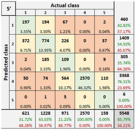
Figure 6.
Confusion matrix corresponding to a time horizon of 5 min.
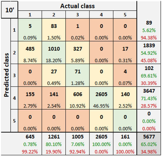
Figure 7.
Confusion matrix corresponding to a time horizon of 10 min.
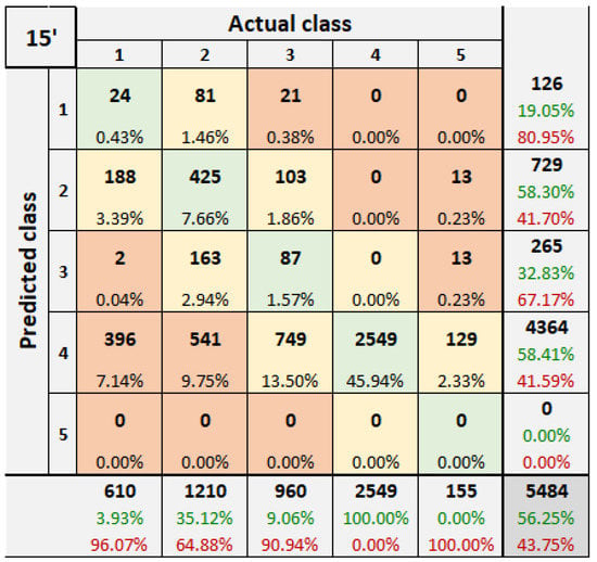
Figure 8.
Confusion matrix corresponding to a time horizon of 15 min.
Figure 6 represents the confusion matrix calculated over a time horizon of 5 min. The overall accuracy level achieved is equal to 65.79% of samples correctly classified. Figure 7 represents the confusion matrix calculated over a time horizon of 10 min. The accuracy obtained over this time horizon is equal to 65.02%. Figure 8 represents the confusion matrix calculated over a time horizon of 15 min. Considering this time horizon, only 56.25% of the total number of samples are correctly classified. It is observable that class 1 (the most populated one) is always recognized without committing any error, while class 5 (the least populated one) is not recognized at all by the model. As expected, the accuracy of classification decreases when the time horizon considered increases. In further detail, the recorded performance drop is very limited when increasing the time horizon from 5 to 10 min (lower than 1%), while it is significant when increasing the time horizon from 10 to 15 min (almost 9%).
Figure 9, Figure 10 and Figure 11 report the sorted daily classification performances for each of the considered time horizons (5, 10, and 15 min), from the best to the worst. Therefore, all the daily classification performances, from the best to the worst, can be observed. In all the diagrams, the average performance level is highlighted by an orange dotted line. In this way, the daily performances above and below the average level can be clearly identified.
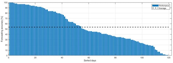
Figure 9.
Sorted daily forecasting performance corresponding to a time horizon of 5 min.
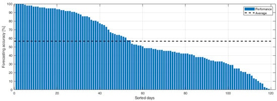
Figure 10.
Sorted daily forecasting performance corresponding to a time horizon of 10 min.
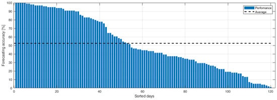
Figure 11.
Sorted daily forecasting performance corresponding to a time horizon of 15 min.
As observed, in a few cases, all the samples are correctly classified, reaching peaks of 100% in the daily classification accuracy. On the other hand, there are days characterized by a very low classification accuracy, where only a bunch of samples are correctly classified.
4. Conclusions
The present work proposed a new nowcasting method to calculate the variability of solar irradiation over multiple time horizons, namely 5, 10, and 15 min ahead. The method was implemented through a Convolutional Neural Network (CNN) that uses the infrared sky images captured by an All-Sky Imager (ASI) installed at the SolarTechLAB, Politecnico di Milano, as input. The implemented system requires two main input elements: the full-sky camera and a computer capable of processing the images. The SkyCam costs EUR 60 k (EUR 45 k for the purchase of a second-hand instrument), while 1 year’s rental costs about EUR 15–20 k. The computer with GPU for image processing costs about EUR 1.5–3 k considering the required technical characteristics. The network’s output consists of a range of possible values of the Clear-Sky Index (CSI), a parameter that considers the effect of transient clouds on the Global Horizontal Irradiation (GHI) only. The available infrared images undergo specific preprocessing, aimed at isolating the region surrounding the position of the sun. In addition, a cleaning procedure has been implemented to exclude rainy conditions from the data involved in the development of the CNN, then the forecast model was tested. The CNN exhibited a discrete performance level, with an accuracy peak over the 5 min time horizon, where 65.79% of the available samples are attributed to the correct range of CSI values. Considering larger forecast horizons, as expected, the overall classification accuracy decreases to 65.02% (10 min forecast horizon) and 56.25% (15 min forecast horizon).
Future works in this area can analyze the effect of introducing some meteorological input parameters. These data, in fact, can help nowcasting because they provide information, such as the current irradiation, very correlated with the CSI to be predicted, and the current wind direction, which can help CNN identify when clouds can cover the sun.
Author Contributions
A.N., E.O. and S.L.; Data curation, A.N.; Formal analysis, A.N., S.O., A.M., E.O. and S.L.; Investigation, E.O.; Methodology, A.N., S.O., A.M. and E.O.; Project administration, S.L.; Software, S.O.; Supervision, A.N. and S.L.; Validation, S.O. and A.M.; Visualization, A.M.; Writing—original draft, A.N., S.O., A.M., E.O. and S.L.; Writing—review and editing, A.N., S.O., A.M., E.O. and S.L. All authors have read and agreed to the published version of the manuscript.
Funding
This research received no external funding.
Institutional Review Board Statement
Not applicable.
Informed Consent Statement
Not applicable.
Data Availability Statement
Supporting data is not available.
Conflicts of Interest
The authors declare no conflict of interest.
References
- Şener, Ş.E.C.; Sharp, J.L.; Anctil, A. Factors impacting diverging paths of renewable energy: A review. Renew. Sustain. Energy Rev. 2018, 81, 2335–2342. [Google Scholar] [CrossRef]
- Kabir, E.; Kumar, P.; Kumar, S.; Adelodun, A.A.; Kim, K.H. Solar energy: Potential and future prospects. Renew. Sustain. Energy Rev. 2018, 82, 894–900. [Google Scholar] [CrossRef]
- Blaschke, T.; Biberacher, M.; Gadocha, S.; Schardinger, I. ‘Energy landscapes’: Meeting energy demands and human aspirations. Biomass Bioenergy 2013, 55, 3–16. [Google Scholar] [CrossRef] [PubMed] [Green Version]
- Kratschmann, M.; Dütschke, E. Selling the sun: A critical review of the sustainability of solar energy marketing and advertising in Germany. Energy Res. Soc. Sci. 2021, 73, 101919. [Google Scholar] [CrossRef]
- Leva, S.; Nespoli, A.; Pretto, S.; Mussetta, M.; Ogliari, E.G.C. PV plant power nowcasting: A real case comparative study with an open access dataset. IEEE Access 2020, 8, 194428–194440. [Google Scholar] [CrossRef]
- Majidpour, M.; Nazaripouya, H.; Chu, P.; Pota, H.R.; Gadh, R. Fast univariate time series prediction of solar power for real-time control of energy storage system. Forecasting 2019, 1, 107–120. [Google Scholar] [CrossRef] [Green Version]
- Yang, D.; Kleissl, J.; Gueymard, C.A.; Pedro, H.T.; Coimbra, C.F. History and trends in solar irradiance and PV power forecasting: A preliminary assessment and review using text mining. Sol. Energy 2018, 168, 60–101. [Google Scholar] [CrossRef]
- Kaur, A.; Nonnenmacher, L.; Pedro, H.T.; Coimbra, C.F. Benefits of solar forecasting for energy imbalance markets. Renew. Energy 2016, 86, 819–830. [Google Scholar] [CrossRef]
- Monjoly, S.; André, M.; Calif, R.; Soubdhan, T. Forecast horizon and solar variability influences on the performances of multiscale hybrid forecast model. Energies 2019, 12, 2264. [Google Scholar] [CrossRef] [Green Version]
- Bird, L.; Milligan, M.; Lew, D. Integrating Variable Renewable Energy: Challenges and Solutions; Technical Report; National Renewable Energy Lab. (NREL): Golden, CO, USA, 2013.
- Kleissl, J. Solar Energy Forecasting and Resource Assessment; Academic Press: New York, NY, USA, 2013. [Google Scholar]
- Zhang, J.; Hodge, B.M.; Florita, A.; Lu, S.; Hamann, H.F.; Banunarayanan, V. Metrics for Evaluating the Accuracy of Solar Power Forecasting; Technical Report; National Renewable Energy Lab. (NREL): Golden, CO, USA, 2013.
- Inman, R.H.; Pedro, H.T.; Coimbra, C.F. Solar forecasting methods for renewable energy integration. Prog. Energy Combust. Sci. 2013, 39, 535–576. [Google Scholar] [CrossRef]
- Leva, S.; Dolara, A.; Grimaccia, F.; Mussetta, M.; Ogliari, E. Analysis and validation of 24 h ahead neural network forecasting of photovoltaic output power. Math. Comput. Simul. 2017, 131, 88–100. [Google Scholar] [CrossRef] [Green Version]
- Niccolai, A.; Nespoli, A. Sun Position Identification in Sky Images for Nowcasting Application. Forecasting 2020, 2, 488–504. [Google Scholar] [CrossRef]
- Polo, J.; Martín-Pomares, L.; Sanfilippo, A. Solar Resources Mapping: Fundamentals and Applications; Springer: Berlin, Germany, 2019. [Google Scholar]
- Kannari, L.; Kiljander, J.; Piira, K.; Piippo, J.; Koponen, P. Building Heat Demand Forecasting by Training a Common Machine Learning Model with Physics-Based Simulator. Forecasting 2021, 3, 290–302. [Google Scholar] [CrossRef]
- Ramirez, L.; Vindel, J. Forecasting and nowcasting of DNI for concentrating solar thermal systems. Adv. Conc. Sol. Therm. Res. Technol. 2017, 293–310. [Google Scholar]
- Shaffery, P.; Habte, A.; Netto, M.; Andreas, A.; Krishnan, V. Automated construction of clear-sky dictionary from all-sky imager data. Sol. Energy 2020, 212, 73–83. [Google Scholar] [CrossRef]
- Richardson, W.; Krishnaswami, H.; Vega, R.; Cervantes, M. A low cost, edge computing, all-sky imager for cloud tracking and intra-hour irradiance forecasting. Sustainability 2017, 9, 482. [Google Scholar] [CrossRef] [Green Version]
- Nouri, B.; Kuhn, P.; Wilbert, S.; Hanrieder, N.; Prahl, C.; Zarzalejo, L.; Kazantzidis, A.; Blanc, P.; Pitz-Paal, R. Cloud height and tracking accuracy of three all sky imager systems for individual clouds. Sol. Energy 2019, 177, 213–228. [Google Scholar] [CrossRef] [Green Version]
- Zhang, J.; Verschae, R.; Nobuhara, S.; Lalonde, J.F. Deep photovoltaic nowcasting. Sol. Energy 2018, 176, 267–276. [Google Scholar] [CrossRef] [Green Version]
- Wang, Y.; Tan, H.; Wu, Y.; Peng, J. Hybrid electric vehicle energy management with computer vision and deep reinforcement learning. IEEE Trans. Ind. Inform. 2020, 17, 3857–3868. [Google Scholar] [CrossRef]
- Fang, X.; Yuan, Z. Performance enhancing techniques for deep learning models in time series forecasting. Eng. Appl. Artif. Intell. 2019, 85, 533–542. [Google Scholar] [CrossRef]
- Voyant, C.; Notton, G.; Kalogirou, S.; Nivet, M.L.; Paoli, C.; Motte, F.; Fouilloy, A. Machine learning methods for solar radiation forecasting: A review. Renew. Energy 2017, 105, 569–582. [Google Scholar] [CrossRef]
- Page, J. The role of solar-radiation climatology in the design of photovoltaic systems. In Practical Handbook of Photovoltaics; Elsevier: Amsterdam, The Netherlands, 2012; pp. 573–643. [Google Scholar]
- Ineichen, P. Validation of models that estimate the clear sky global and beam solar irradiance. Sol. Energy 2016, 132, 332–344. [Google Scholar] [CrossRef] [Green Version]
- Marty, C.; Philipona, R. The clear-sky index to separate clear-sky from cloudy-sky situations in climate research. Geophys. Res. Lett. 2000, 27, 2649–2652. [Google Scholar] [CrossRef]
- Liu, H.; Chen, C.; Lv, X.; Wu, X.; Liu, M. Deterministic wind energy forecasting: A review of intelligent predictors and auxiliary methods. Energy Convers. Manag. 2019, 195, 328–345. [Google Scholar] [CrossRef]
- Butt, H.; Raza, M.R.; Ramzan, M.J.; Ali, M.J.; Haris, M. Attention-Based CNN-RNN Arabic Text Recognition from Natural Scene Images. Forecasting 2021, 3, 520–540. [Google Scholar] [CrossRef]
- Menculini, L.; Marini, A.; Proietti, M.; Garinei, A.; Bozza, A.; Moretti, C.; Marconi, M. Comparing Prophet and Deep Learning to ARIMA in Forecasting Wholesale Food Prices. Forecasting 2021, 3, 644–662. [Google Scholar] [CrossRef]
Publisher’s Note: MDPI stays neutral with regard to jurisdictional claims in published maps and institutional affiliations. |
© 2022 by the authors. Licensee MDPI, Basel, Switzerland. This article is an open access article distributed under the terms and conditions of the Creative Commons Attribution (CC BY) license (https://creativecommons.org/licenses/by/4.0/).