Examining Deep Learning Architectures for Crime Classification and Prediction

Abstract

In this paper, a detailed study on crime classification and prediction using deep learning architectures is presented. We examine the effectiveness of deep learning algorithms in this domain and provide recommendations for designing and training deep learning systems for predicting crime areas, using open data from police reports. Having time-series of crime types per location as training data, a comparative study of 10 state-of-the-art methods against 3 different deep learning configurations is conducted. In our experiments with 5 publicly available datasets, we demonstrate that the deep learning-based methods consistently outperform the existing best-performing methods. Moreover, we evaluate the effectiveness of different parameters in the deep learning architectures and give insights for configuring them to achieve improved performance in crime classification and finally crime prediction.

1. Introduction

Predictive policing is the use of analytical techniques to identify likely places of future crime scenes or past crime perpetrators, by applying statistical predictions [1]. As a crime typically involves a perpetrator and a target and occurs at a certain place and time, techniques of predictive policing need to answer: (a) who will commit a crime, (b) who will be offended, (c) what type of crime, (d) in which location and (e) at what time a new crime will take place. This work does not focus on the victim and the offender, but on the prediction of when and where a certain crime type will occur, using past data.

The ultimate goal, in a policing context, is the selection of the top areas in the city for the prioritisation of law enforcement resources per department. One of the most challenging issues of police departments is to have accurate crime forecasts to dynamically deploy patrols and other resources to improve deterring of crime occurrence and police response times.

Routine activity theory [2] suggests that most crimes take place when three conditions are met: a motivated offender, a suitable victim and lack of victim protection. The rational choice theory [3], suggests that prospective criminal weights the gain of successfully committing the crime against the probability of being caught and makes a rational choice whether to actually commit the crime or not. Both theories agree that a crime takes place when a person willing to commit it has an opportunity to do so. As empirical studies in near repeat victimisation [4,5,6,7] have shown, these opportunities are not randomly distributed but follow patterns in both space and time. Traditionally, police officers use maps of an area and place a pin on the map for every reported incident. Studying these maps, they can detect these patterns and, thus, efficiently predict hotspots; the areas with the higher possibility for a crime to occur, compared to the neighbouring areas.

Simple mapping methods are not sufficient to make use of these general phenomena as early indicators for predicting crimes but more complex methodologies, such as machine learning, are needed. Various machine learning methodologies like Random Forests [8], Naive Bayes [9] and Support Vector Machines (SVMs) [10] have been exploited in the literature both for predicting the number of crimes that will occur in an area and for hotspot prediction. The success of a machine learning analysis highly depends on the experience of the analyst to prepare the data and to hand-craft features that describe properly the problem in question.

Deep learning (DL) is a machine learning approach where the algorithm can extract the features from the raw data, overcoming the limitations of other machine learning methodologies. Of course, this benefit comes at a high price in computational complexity and demand in raw data. This global research trend was picked recently by Wang et al. [11] for predicting hourly fluctuations in crime rates. Building on this very interesting work, we investigate DL architectures for crime hotspot prediction and present design recommendations. The major contributions of this paper are

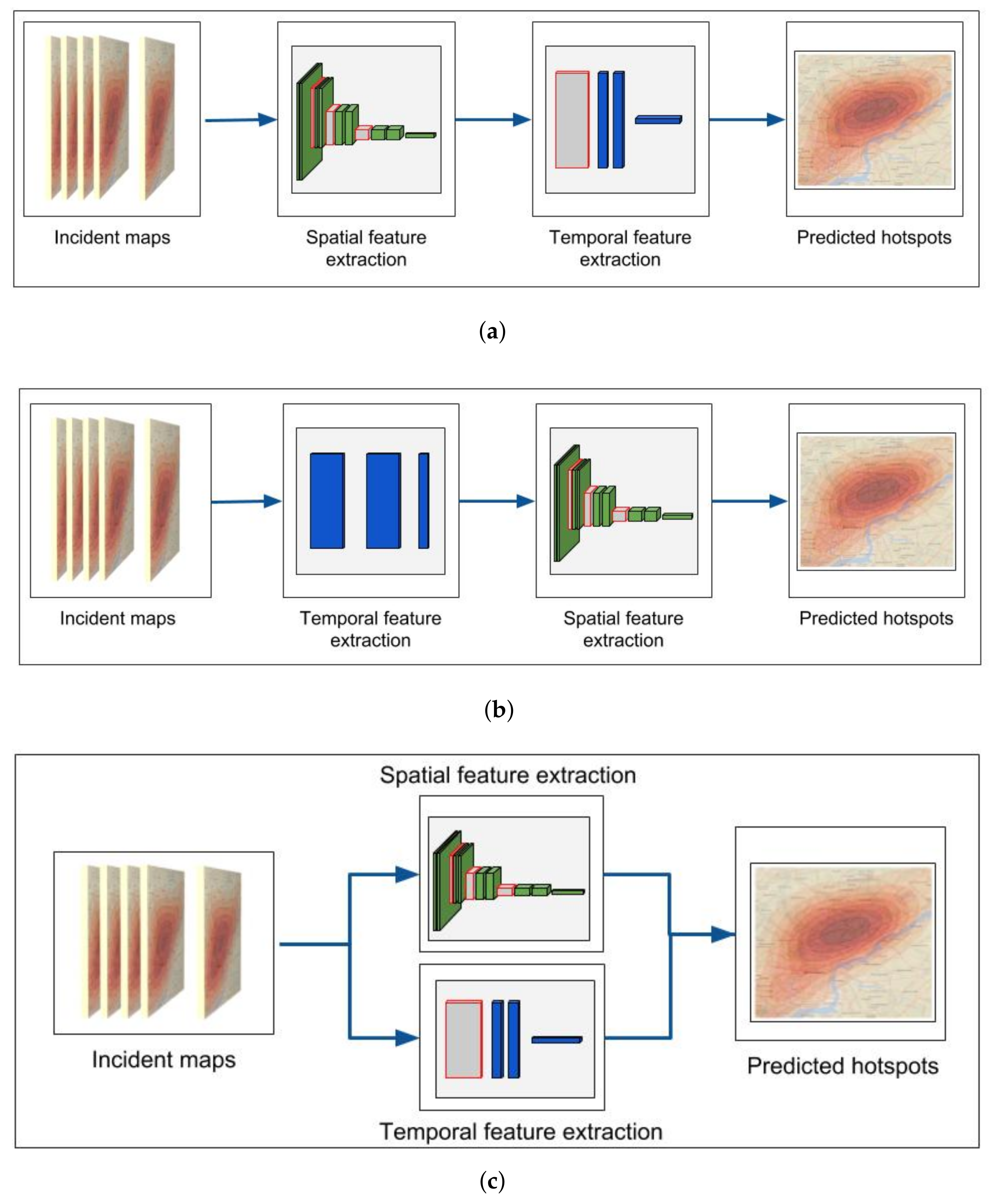
• We present 3 fundamental DL architecture configurations for crime prediction based on encoding: (a) the spatial and then the temporal patterns, (b) the temporal and then the spatial patterns, (c) temporal and spatial patterns in parallel.
• We experimentally evaluate and select the most efficient configuration to deepen our investigation.
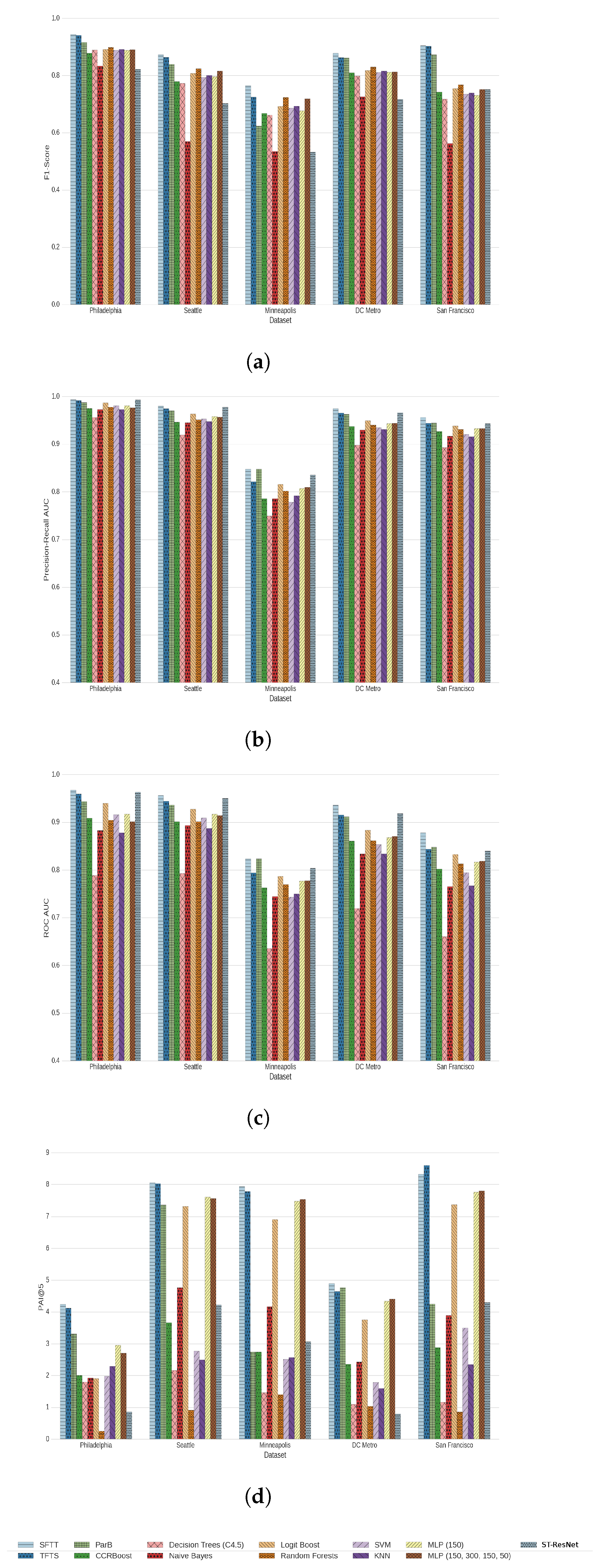
• We compare our models with 10 state-of-the-art algorithms on 5 different crime prediction datasets that contain more than 10 years of crime report data.
• Finally, we propose a guide for designing DL models for crime hotspot prediction and classification.

The rest of the paper is organised as follows: Section 2, discusses the related work on crime prediction and classification as well as recent developments in deep learning approaches for spatio-temporal data. Section 3, formulates the problem in question. Section 4, discusses the proposed methods for applying DL in crime prediction and classification. Section 5 presents the baseline approaches, the datasets used and the metrics to measure the effectiveness of each model. In Section 6, the presentation and discussion of results in different configurations and parameters are conducted. Finally, Section 7, draws conclusions and propose new exploration paths to be investigated in the future.

2. Related Work

Criminology literature investigates the relationship between crime and various features, developing approaches for crime forecasting. The majority of the works focus on the prediction of hotspots, which are areas of varying geographical size with high crime probability. The methods include Spatial and Temporal Analysis of Crime (STAC) [12], Thematic Mapping [13] and Kernel Density Estimation (KDE) [14].

In STAC, the densest concentrations of points on the map are detected and then fit a standard deviational ellipse for each one. Through the study of the size and the alignment of the ellipses, the analyst can draw conclusions about the nature of the underlying crime clusters [15].

In Thematic Mapping, the map is split into boundary areas while offences are placed as points on a map. The points can then be aggregated to geographic unit areas and shaded in accordance with the number of crimes that fall within [13]. This technique enables quick determination of areas with a high incidence of crime and allows further analysis of the problem by “zooming in” on those areas. Boundary areas can be arbitrarily defined, using i.e., police beats, enabling linking of crime with other data sources, such as population.

Owing to the varying size and shape of most geographical boundaries, thematic mapping can be misleading in identifying the existence of the highest crime concentrations [16]. Hence, this technique can fail to reveal patterns across and within the geographical division of boundary areas [17]. KDE divides the area in a regular grid of cells and estimates a density value for each cell, using a kernel function that estimates the probability density of the actual crime incidents [18,19]. The resulting two-dimensional scalar can then be used to create a heatmap, affected by the cell size, the bandwidth and the kernel function used [20].

All three above mentioned methods solely rely on the spatial dimension of incidents. On the other hand, methods presented by Mohler et al. [21] and Ratcliffe [22], model the temporal dimension of the crime. Mohler et al. propose the use of self-exciting point process to model the crime and gain insights into the temporal trends in the rate of burglary, while Ratcliffe investigates the temporal constraints on crime and proposes an offender travel and opportunity model. These works validate the claim that a proportion of offending is driven by the availability of opportunities presented in Cohen’s routine activity theory [2]. Ghazvini et al. [23] propose a model that can isolate short term repetitiveness, thus allowing the detection of serial crime sprees.

Nakaya and Yano [24], extend the crime cluster analysis with a temporal dimension. They employ the space-time variants of KDE to simultaneously visualise the geographical extent and duration of crime clusters. Taking a step further, Toole et al. [25], use criminal offence records to identify spatio-temporal patterns at multiple scales. They employ various quantitative tools from mathematics and physics and identify significant correlations in both space and time in the crime behavioral data.

Machine learning has also been a popular approach for crime forecasting. Olligschlaeger [26] examines the use of Multi-Layer Perceptrons (MLP) on GIS systems. One of the use cases is the prediction of drug-related calls for service on the 911 call centres of Pittsburgh USA. By superimposing the map area with a grid of cells, Olligschlaeger creates 445 cells of a 2150 sq feet area each. For each cell, 3 call-related early indicators are calculated: (a) the number of weapon-related calls, (b) the number of robbery related calls and (c) the number of assault-related calls that occur in the cell area. Additionally, the proportion of commercial to residential properties in the cell area and a seasonal index are also used as indicators. Due to the lack of processing power in 1997, the MLP neural network that was used had a mere 9 neurons in a single hidden layer.

Kianhmer and Alhajj [27] use SVMs in a machine learning approach of hotspot location prediction. The success of SVMs is re-examined by Yu et al. [28] in comparison to other machine learning approaches like Naive Bayes and Random Forests. They observe that in the case of residential burglary, what has happened in a particular place is likely to reoccur.

Gorr and Olligschlaeger compare different regression approaches for predicting a set of crime categories using data from Pittsburgh [29]. They run regressions of different complexity on the same data set and compare the results. They found that simple time series were outperformed by more sophisticated methods. In particular, they found that by using a smoothing coefficient (i.e., applying increased weight on recent data) the predicted mean absolute percent error is improved.

On the other hand, Feng et al. [30] applied the Prophet model on crime occurrence datasets from 3 major cities in the US and concluded that time series models can in fact outperform neural networks. Their models detected a 3-year seasonality in crime trends.

Eftelioglu et al. [31], propose a method to detect ring-shaped hotspots. In some types of crime, like burglaries, serial offenders remain in a certain area because of familiarity with this region while on the other hand, proximity to their home could compromise their anonymity, leading to a high concentration of incidents inside a ring-shaped area centred to the outbreak point.

Xu et al. [32], combine online learning with ensemble methods for their spatiotemporal forecast framework. This framework estimates the optimal weights for combining the ensemble member forecasts. Moreover, it uses an “online” algorithm that revises its previous forecasts when a future forecast is incorrect.

Yu et al. [33] propose a new approach to identify the hierarchical structure of spatio-temporal patterns at different resolution levels and subsequently construct a predictive model based on the identified structure. They first obtain indicators within different spatio-temporal spaces and construct distributed spatio-temporal patterns (DSTP). Next, they use a greedy searching and pruning algorithm to combine the DSTPs to form an ensemble spatio-temporal pattern (ESTP). The model, named CCRBoost, combines multiple layers of weighted ESTPs. They tested this method in predicting residential burglary, achieving 80% accuracy on a non-publicly available dataset.

Recently, Wang et al. [11] propose the use of deep learning for the prediction of hourly crime rates. In particular, their model ST-ResNet extends the ResNet [34] model for use in spatio-temporal problems like crime forecasting. They detected that future crime rates depend on the trend set in the previous week, the time of day and the nearby events both in space and in time. For each one of these contributing factors, they use a separate ResNet model that offers a prediction based on indicators of a weekly period, a daily period and an hourly period respectively. The outputs of the 3 models are combined to form a common prediction. They also use external features like day of month, day of week and hour of day to get a more accurate prediction.

Wang et al. propose a methodology very similar to Simonyan and Zisserman [35]. Motivated by the fact that videos can be naturally decomposed into spatial and temporal components, Simonyan and Zisserman propose a two-stream approach that breaks down the learning of video representation by using one stream to learn spatially and the other stream to learn temporal clues. For the spatial stream, they adopt a typical CNN architecture using raw RGB images as input to detect appearance information. To account for temporal clues among adjacent frames, they explicitly generate multiple-frame dense optical flows derived from computing displacement vector fields between those frames.

Since this temporal stream operates on adjacent frames, it can only depict movements within a short time window. The second and most important problem of this method is that the order of the frames is not taken into account. Both problems are addressed by Wu et al. [36], by replacing the temporal CNN stream with a Long-Short Term Memory (LSTM) [37] network, thus leveraging long term temporal dynamics. By fusing the outputs of the two streams, they jointly capture spatial and temporal features for video classification. They observed that CNNs and LSTMs are highly complementary. According to Ruta et al. [38] high complementarity of methods leads to ensemble methods that have excellent generalisation ability.

3. Problem Formulation

Let D be the dataset of n four-dimensional vectors $x_i$ with $i\in \{1,n\}$ where each $x_i$ contains information on the location (longitude and latitude), the time and the type of a reported crime (crime category). It is typical in the literature to aggregate the spatial information by splitting the city map in a two-dimensional grid with cell edge size l, so that a p cells square grid is produced (e.g., given an 8 km by 8 km sized map and a cell edge size $l=500$ m, $p=16$ is calculated and thus a $16\times 16$ cells grid is produced).

Next, the $x_i$ data points are aggregated in each corresponding cell as a sum of occurrences of a certain crime type. Moreover, since the data are time-series of data points, the data are also split in time windows of duration t and create multiple aggregated incident maps I for the whole period T of the time-series.

Our goal is to classify each cell as a hotspot or not for a certain type of crime with the highest possible spatial resolution in a neighbourhood of the monitored city. Additionally, the hotspots that are predicted should be ranked according to the number of crimes that will occur inside their area for prioritising and allocating policing resources more efficiently. To enhance the probability of an area being predicted as a hotspot, we use secondary parallel prediction of the number of occurrences y for each crime.

Accordingly, the problem is defined as (a) a binary classification of the cells that will have an occurrence of a certain crime in a certain time window in the future; (b) the probability that a crime is classified as a hotspot is dependant on the number of occurrences y of a certain crime for each cell in the defined future time window.

4. Proposed Methodology

CNNs consist of convolutional layers, characterised by an input map I, a bank of filters K and biases b, producing an output map O. In the case of crime maps, by aggregating the crime incidents ${\mathbf{x}}_i$ to cells for every incident type and timespan t, we produce an ordered collection of incident maps I for the whole duration T, with height h, width w and c channels such that $I\in {\mathbb{R}}^{h\times w\times c}$, analogous to a sequence of image frames from a video. Subsequently, for a bank of d filters with size $k_1$ and $k_2$, we have $K\in {\mathbb{R}}^{k_1\times k_2\times c\times d}$ and biases $b\in {\mathbb{R}}^d$, one for each filter. The output map $O\in {\mathbb{R}}^{h\times w\times d}$ is calculated by applying:

$$O_{ij}=\sum _{m=0}^{k_1-1}\sum _{n=0}^{k_2-1}\sum _{c=0}^C{K}_{m,n,c}·I_{i+m,j+n,c}+b$$

(1)

for every $i\in \{1,H-k_1\}$, $j\in \{1,W-k_2\}$, for each filter.

LSTMs, are a variant of RNNs that are better suited to long sequences since they do not suffer from the vanishing gradient effect [37]. An LSTM cell, maps the input vector $x^{\left(t\right)}\in {\mathbb{R}}^n$ for each timestep t to the output vector $h^{\left(t\right)}\in {\mathbb{R}}^m$, by recursively computing the activation of the units in the network using the following equations:

$$\begin{array}{cc}\hfill i^{\left(t\right)}& =\sigma (W_{xi}{x}^{\left(t\right)}+W_{hi}{h}^{(t-1)}+W_{hi}{h}^{\left(t\right)}+b_i)\hfill \\ \hfill f^{\left(t\right)}& =\sigma (W_{xf}{x}^{\left(t\right)}+W_{hf}{h}^{\left(t\right)}+W_{hf}{h}^{\left(t\right)}+b_f)\hfill \\ \hfill c^{\left(t\right)}& =f^{\left(t\right)}{c}^{(t-1)}+i_{t}tanh(W_{xc}{x}^{\left(t\right)}+W_{hc}{h}^{\left(t\right)}+b_c)\hfill \\ \hfill o^{\left(t\right)}& =\sigma (W_{xo}{x}^{\left(t\right)}+W_{ho}{h}^{(t-1)}+W_{ho}{h}^{\left(t\right)}+b_o)\hfill \\ \hfill h^{\left(t\right)}& =o^{\left(t\right)}tanh\left(c^{\left(t\right)}\right)\hfill \end{array}$$

(2)

where $x^{\left(t\right)}$ and $h^{\left(t\right)}$ are the input and output vectors, $i^{\left(t\right)}$, $f^{\left(t\right)}$, $c^{\left(t\right)}$, $o^{\left(t\right)}$ are respectively the activation vectors of the input gate, forget gate, memory cell and output gate, and $W_{ab}$ denote the weight matrix from a to b. In each time step t, the input of the LSTM cell consists of the input vector $x^{\left(t\right)}$ at time t and the output vector $h^{(t-1)}$ from time step $t-1$.

Based on the methodology of Wu et al. combination of CNNs and RNNs can be jointly used for a spatiotemporal forecasting model. Depending on the order that CNNs and LSTMs are used, 3 approaches present themselves.

The first approach, named SFTT (Figure 1a), passes each incident map from a CNN submodel, producing a feature vector for every timespan t that encodes the spatial distribution of incidents in a feature space that is much smaller than the original. The sequence of $\frac{T}{t}$ feature vectors is then fed into the LSTM network which can extract temporal features. All 11 crime categories are used as input for the incident maps in separate input channels. The intuition is that the ratio of crime types in each area encodes implicitly the socioeconomic status and activities’ profile of the area and thus provides better modelling of the situation. The justification is presented in Section 6.3.

The second approach is to input the feature maps to an RNN submodel for temporal feature extraction and then use a CNN for spatial features. For this approach, named TFTS (Figure 1b), we firstly extract a temporal feature vector for each cell by passing each sequence of incidents ${\mathbf{x}}_i$ of each cell through an LSTM network model. The extracted temporal features for each cell retain the relative position on the monitored area (i.e., their cell position), thus temporal maps of the area are created. The temporal maps are then used as input features that are fed to a CNN network for spatial information extraction.

The third possibility is to extract spatial and temporal features in parallel, named ParB (Figure 1c), using 2 separate branches. The output of the 2 branches can be combined so that prediction accounts for both groups of features.

For the spatial feature extraction, we explore four possible body architectures depicted in Figure 2. Three out of them are based on VGGNet [39], ResNet [34] and FastMask [40], respectively, while the fourth one is a combination of the ResNet and the FastMask models. All these models were originally designed to extract features from images of size $224\times 224$ pixels. To follow the grid resolution ranges used in related crime prediction papers [15,16,17,33], the input grid resolution had to be reduced. Thus, similar models but with smaller input and fewer parameters were implemented.

A common practice in DL is to take models that are trained in one dataset and use them in another dataset, sometimes even in different domains. One reason that we did not use the ImageNet [41] pre-trained models of VGG, ResNet and FastMask are that we altered the models themselves. Another reason is that the ImageNet dataset is not only of a different domain but the structural and statistical characteristics of images are completely different than incident maps that a random start is preferred.

In our VGGNet body, we use series of 5 pairs of convolution layers, where the first 3 are followed by pooling layers. In the first 4 pairs of the convolution layers, the filter size we use is $3\times 3$, while in the last pair the filter size is $1\times 1$. The first 2 pairs of convolutions apply 32 filters, the following 2 pairs apply 64 filters and the last pair applies 256 filters. In all convolution function layers, the activation function is the Rectified Linear Units (ReLU), which allows the networks to converge faster [39]. The pooling layers use the max operation. We use a Batch Normalisation layer and a Dropout layer after each pooling layer as our datasets are fairly small and the possibility of overfitting is significant. The complete CNN body of this network is depicted in Figure 2a.

A more complex CNN that has proven to be more effective in extracting spatial information in image classification than VGGNet is ResNet [34]. In ResNet, the added residual layers aim to solve the degradation problem that was encountered when the convolutional networks became too deep. In every convolution block, there is a shortcut connection added to each pair of $3\times 3$ filters. Inspired by this tactic, we modified the feature extractor to incorporate residual connections as shown in Figure 2b. In each block, we use 3 convolution layers with $3\times 3$, $1\times 1$ and $3\times 3$ sized filters and a parallel residual convolution layer with a filter size of $3\times 3$. In each consecutive block, the number of filters in the last convolution layer and the residual layer is doubled with regard to the previous block. The number of filters in the first 2 convolution layers is a quarter of the last. The output of the block layers with the output of the residual layer is then averaged before a max-pooling layer changes the scale.

In FastMask [40], Hu et al. use a block of convolutional layers (called a neck) to extract features of different scales. The features are then concatenated before they are forwarded to the next neck. The output of all the necks is also concatenated before being passed on to the classification layers. To change scale, in each neck, there is an average pooling layer. Each neck has 2 paths for information to flow. In the one path, the input of the neck is passed through an average pooling layer, thus zooming out without extracting any new features. The other path uses 2 convolutional layers with $3\times 3$ sized filters, extracting this way a number of features from this scale. In Figure 2c, we illustrate our own implementation of the FastMask model.

The two methods differ in their philosophy of using residual information. In ResNet, the blocks are used sequentially, while in FastMask the outputs of all blocks are brought together in one last concatenation layer. Moreover, the residual information is averaged with the new features in the ResNet design, while in FastMask the residual information is concatenated to the newly extracted features. By using the blocks of ResNet in the place of FastMask necks, we create a variation where averaged main and residual features from each scale are then concatenated (Figure 2d).

The temporal feature extraction in the first approach is achieved by extracting the temporal correlations in the sequence of vectors holding the spatial features by using an LSTM submodel. This LSTM model consists of 3 consecutive LSTM layers where the 2 first ones have 500 neurons each, while the last one has the same number of neurons as the number of cells that the model predicts. In the second and third approaches, an LSTM submodel with 3 layers of 32 neurons is applied to each cell of the input. Each LSTM layer adds another level of non-linearity in the extraction of temporal patterns from the input data.

In all proposed models, the extracted spatio-temporal features are finally fed into two parallel fully connected output layers. On the one output layer we use the binary cross-entropy (BCE) loss function to classify each cell as a hotspot or not:

$$BCE=-\frac{1}{N}\sum _i^N[{\widehat{o}}_{i}log{o}_i+(1-{\widehat{o}}_i)log(1-o_i)]$$

(3)

where N is the total number of cells, ${\widehat{o}}_i$ is the predicted class of cell i and $o_i$ is the actual class of cell i.

On the other output layer we apply the mean squared error (MSE) loss function:

$$MSE=-\frac{1}{N}\sum _i^N{(y_i-{\widehat{y}}_i)}^2$$

(4)

where N is the total number of cells, ${\widehat{y}}_i$ is the predicted number of crimes that will occur in the cell during the target time period and $y_i$ is the actual number of crimes that occurred inside cell i during the target time period.

The loss from both outputs is combined during the backpropagation step so that the spatio-temporal features that are extracted, affected by the classification of a cell as a hotspot and to the number of crimes that occurred within the cell. This approach was selected to drive the final classifier to give bigger probabilities to cells where multiple crimes occur.

By changing the binary cross-entropy loss function to the equivalent multi-class cross-entropy (Equation (5)), we are able to predict the hotspot distribution for all the crimes at the same network.

$$MCCE=-\frac{1}{N}\sum _i^N\sum _k^C[{\widehat{o}}_{ik}log{o}_{ik}]$$

(5)

5. Experimental Setup

5.1. Algorithms

To have a proper assessment of the capability of the DL methods, we compare them with the state-of-the-art CCRBoost [33] and ST-ResNet [11] methods, as well as eight baseline methodologies that commonly appear in the recent relevant literature.

• CCRBoost [33]. CCRBoost starts with multi-clustering followed by local feature learning processes to discover all possible distributed patterns from distributions of different shapes, sizes, and time periods. The final classification label is produced using groupings of the most suitable distributed patterns.
• ST-ResNet [11]. The original ST-ResNet model uses 3 submodels with residual connections, which each has 4 input channels in parallel, to extract indicators from 3 trends: previous week, time of day and recent events. In our problem, the temporal resolution is not hourly but daily so the 3 periods are replaced by day of month, day of week and recent events equivalently.
• Decision Trees(C4.5) [42] using confidence factor of 0.25; Decision Trees is a non-parametric supervised learning method that predicts the value of a target variable by learning simple decision rules inferred from the data features.
• Naive Bayes [9] classifier with a polynomial kernel; Naive Bayes methods are a set of supervised learning algorithms based on applying Bayes’ theorem with the “naive” assumption of independence between every pair of features.
• LogitBoost [43] using 100 as its weight threshold; The LogitBoost algorithm uses Newton steps for fitting an additive symmetric logistic model by maximum likelihood.
• Random Forests [8] with 10 trees; A random forest is a meta estimator that fits a number of decision tree classifiers on various sub-samples of the dataset and use averaging to improve the predictive accuracy and control over-fitting.
• Support Vector Machine (SVM) [10] with a linear kernel; SVMs are learning machines implementing the structural risk minimisation inductive principle to obtain good generalisation on a limited number of learning patterns.
• k Nearest Neighbours [44] with 3 neighbours; kNN is a classifier that makes a prediction based on the majority vote of the k nearest samples on the feature vector space.
• MultiLayer Perceptron (MLP(150)) [26] with one hidden layer of 150 neurons;
• MultiLayer Perceptron (MLP(150, 300, 150, 50)) [45] with four hidden layers of 150, 300, 150 and 50 neurons each;

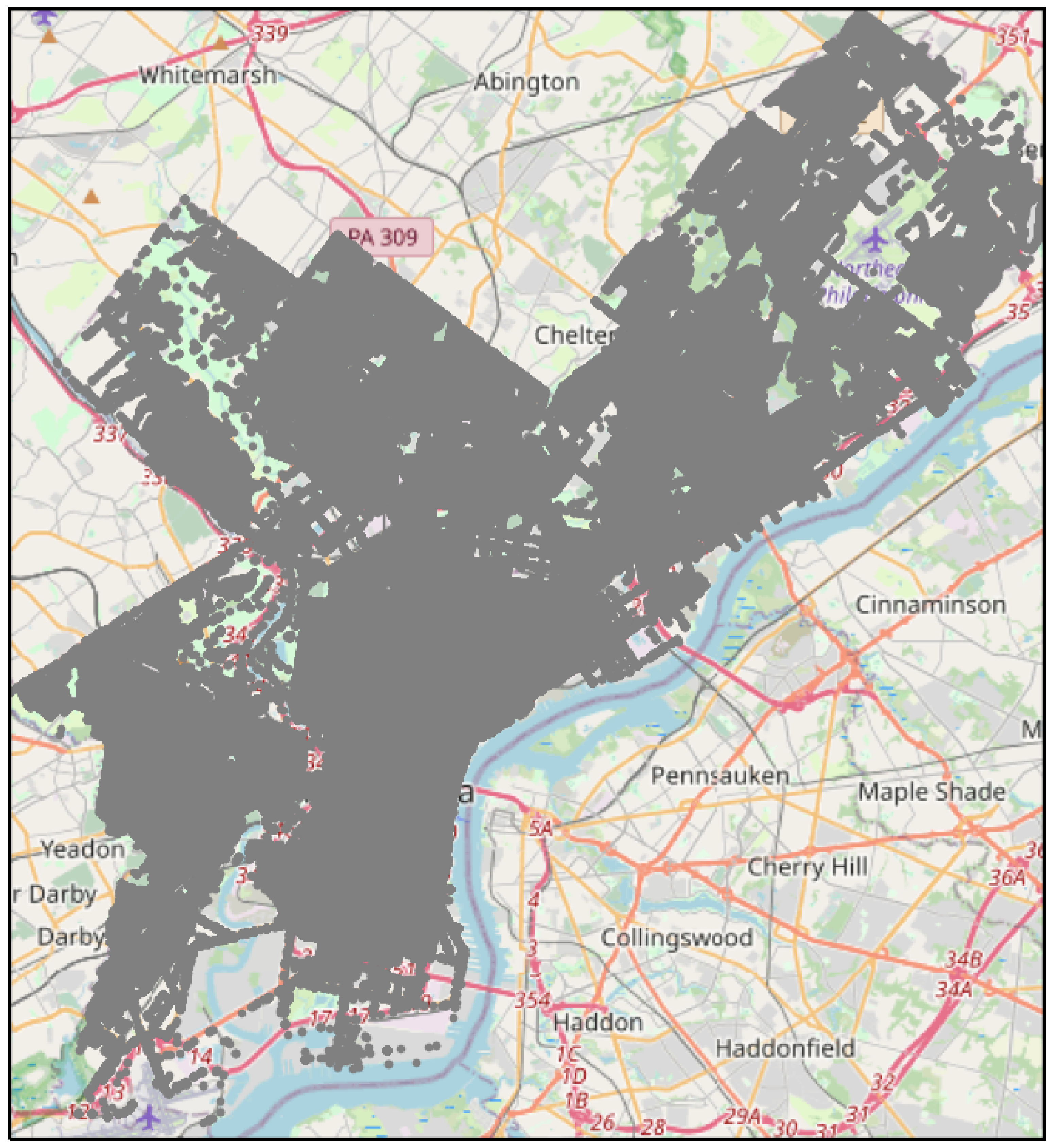
The CCRBoost algorithm was reimplemented by us in python, ST-ResNet is based on DeepST [46] which we downloaded from github (https://github.com/lucktroy/DeepST/tree/master/scripts/papers/AAAI17, accessed on 25 October 2019) and adapted, while for the rest of the baseline methods we used the implementations available from scikit-learn [47]. Our DL experiments were implemented in the Keras framework [48] using the tensorflow [49] backend.

The complexity of the algorithms is compared, in terms of computational time and the number of learnable parameters, in

Table 1. Complexity of all algorithms in total training time for the “All Crimes” crime type in the Philadelphia dataset and number of trainable parameters for the DL architectures.

Algorithm	Training Time	# Parameters
CCRBoost	0:00:38	-
Decision Trees (C4.5)	0:00:02	-
Naive Bayes	0:00:03	-
Logit Boost	0:00:05	-
SVM	0:01:17	-
Random Forests	0:00:03	-
KNN	0:00:02	-
MLP (150)	0:00:13	-
MLP (150, 300, 150, 50)	0:00:24	-
ST-ResNet	0:05:59	1.343.043
SFTT-VGG19	0:48:11	30.117.120
TFTS	0:24:32	10.260.016
ParB	3:15:05	31.942.280
SFTT-ResNet	0:17:53	7.348.899
SFTT-FastMask	0:17:57	6.917.264
SFTT-FastResMask	1:53:09	7.610.299

. The baseline algorithm are typically much faster, however, the DL based ones are also equally applicable since they need minutes of computation to return results. The only exception is SFTT-FastResmask which required approx. 2 h to converge. All experiments were performed on a 12core 3.3 GHz Linux system with 64 GB RAM and an Nvidia TitanX GPU with CUDA [50].

5.2. Datasets

In the last couple of years, a number of new datasets have been published in the field of crime prediction, mainly from law enforcement agencies in the US. In this paper, we have selected and used in our experiments, 5 of the most prominent open datasets that can be downloaded from Kaggle (https://www.kaggle.com/, accessed on 14 May 2018). These 5 datasets include incident reports from Seattle (https://www.kaggle.com/samharris/seattle-crime, accessed on 14 May 2018), Minneapolis (https://www.kaggle.com/mrisdal/minneapolis-incidents-crime, accessed on 14 May 2018), Philadelphia (https://www.kaggle.com/mchirico/philadelphiacrimedata, accessed on 14 May 2018), San Fransisco (https://www.kaggle.com/c/sf-crimedatasets/, accessed on 14 May 2018) and Metropolitan DC (https://www.kaggle.com/vinchinzu/dc-metro-crime-data, accessed on 14 May 2018) police departments. While each dataset contains a number of unique attributes, all 5 datasets report a location (in latitude and longitude), a time and a type of event for each incident ${\mathbf{x}}_i$. The basic information for each dataset is presented in

Table 2. Basic statistics for the 5 examined datasets.

Dataset	Start Year	End Year	Num. of Incidents
Philadelphia	2006	2017	2,203,785
Seattle	1996	2016	684,472
Minneapolis	2010	2016	136,121
DC Metro	2008	2017	313,410
San Francisco	2003	2015	878,049

.

An example plotting of all incidents from 2006 in the Philadelphia dataset is depicted in Figure 3.

Some of the datasets have multiple time attributes recorded, for example, the time when an incident took place and the time when it was reported. Since the report time is recorded by automatic systems, we selected to use this time feature when available. Additionally, the different datasets all use a different system of categorisation for the various reported crime types. To homogenise as much as possible the available data, we assigned each dataset crime type to a common category for all datasets. By doing so we ended up with 10 crime categories that were used in this paper. Details about this methodology are provided in the Appendix A.

The spatial resolution of all datasets is enough for a block-level analysis of crime. Being consistent with the grid resolution ranges that are used in related crime prediction papers [15,16,17,33] the finer block size resolution is defined to have cell edge size $l\approx 450$ m, resulting in grids of $40\times 40$ cells. Using an even finer resolution, the resulting grids would be extremely sparse, especially in crime types with a small number of incidents. The coarser resolution of neighbourhoods has cells with approximate cell edge size $l\approx 800$ m, leading to grids of $16\times 16$ cells. For the different datasets, instead of adjusting the number of cells according to actual distances in the cities, we opted to use a fixed number of cells overlaid on the area under investigation for each dataset.

We aim to create a setting where emerging hotspots are predicted in advance by evaluating past incidents in the current month. Thus, the past incidents are aggregated in incident maps I of timespan t of 1 day, and for a period T of 30 days i.e., 30 daily incident maps are used as input to forecast crimes for the next period. We used a daily timespan to aggregate incidents ${\mathbf{x}}_i$ so that enough temporal detail can be extracted while the time series are sufficiently populated.

The smallest of our datasets describes just over 4 years of data. For this reason, we extracted from all the datasets 3 years of incidents to use as training data and 1 year of incidents for testing purposes. Testing is performed by making a prediction for every month and the reported scores are the mean of the twelve individual prediction scores. The number of samples is relatively small but is enough to evaluate which of the proposed architectures can perform better.

Each cell is marked as a hotspot, if at least one incident occurred in the following month, otherwise a coldspot. After the crime categories are merged, for the training time period, the average number of hotspots per day is presented in

Table 3. Mean number of hotspots per day for every crime type and dataset for the highest resolution of 40 cells by 40 cells.

Crime Type	Philadelphia	Seattle	Minneapolis	DC Metro	San Francisco
ASSAULT	80.28	12.84	3.08	6.32	14.96
THEFT	116.72	21.34	17.46	27.39	40.44
ROBBERY	20.74	2.99	6.13	10.56	4.74
BURGLARY	23.76	17.06	12.36	9.81	8.65
MOTOR VEHICLE	27.94	10.01	14.44	8.43	7.77
ARSON	1.37	0.10	0.32	0.10	0.29
HOMICIDE	0.80	0.03	0.74	0.27	0.0
VICE	4.36	22.59	0.72	0.59	1.59
NARCOTICS	27.90	3.21	0.0	0.0	5.54
OTHER	102.37	40.15	0.09	23.24	51.81
# CELLS	752	818	1123	702	1057

for every crime type. The cells that had no activity in the total duration of the experiments are considered outside the study area and were removed from the metrics calculation. In Table 3, we only present the number of cells that remain inside the study area. From these numbers, we observe that especially in the sparsest crime types there is a class imbalance problem. To avoid it, we have selected metrics that take this fact into account.

5.3. Metrics

When dealing with data that have a class imbalance, the metric of accuracy is not very informative because by always predicting the most dominant class the scores will be very high. $F1score$ is preferred because it is the harmonic mean of precision and recall. Precision is the number of correct positive results divided by the number of all positive results, and recall is the number of correct positive results divided by the number of positive results that should have been returned. The $F1score$ is calculated by

$$F1score=2\ast \frac{precision\ast recall}{precision+recall}$$

(6)

with the $F1score$ we measure the ability of the methods to both correctly predict hotspots and how many of the hotspots we identified at the same time.

$AUROC$ (Area Under Curve—Receiver Operating Characteristic) is the calculated area under a receiver operating characteristic curve. The ROC curve plots parametrically $TPR\left(m\right)$ versus $FPR\left(m\right)$ with m being the probability threshold used to classify a prediction as a hotspot.The $TPR$ (True Positive Rate) and $FPR$ (False Positive Rate) are defined as:

$$TPR=\frac{Tru{e}_{hot}}{Tru{e}_{hot}+Fals{e}_{cold}}$$

(7)

$$FPR=\frac{Fals{e}_{hot}}{Fals{e}_{hot}+Tru{e}_{cold}}$$

(8)

The area under the curve summarises the performance of a classifier for all possible thresholds and is equal to the probability that a classifier will rank a randomly chosen hotspot higher than a randomly chosen coldspot when using normalised units [51].

$$AUROC={\int }_{\infty }^{-\infty }TPR\left(m\right)-{FPR}^{\prime }\left(m\right)dm$$

(9)

$AUCPR$ (Area Under Curve—Precision Recall) equivalently, is the calculated area under a precision-recall curve. A precision recall curve plots parametrically $precision\left(m\right)$ versus $recall\left(m\right)$ with m the varying parameter as above, where:

$$precision=\frac{Tru{e}_{hot}}{Tru{e}_{hot}+Fals{e}_{hot}}$$

(10)

$$recall=\frac{Tru{e}_{hot}}{Tru{e}_{hot}+Fals{e}_{cold}}$$

(11)

PAI (Prediction Accuracy Index), which is defined by Chainey et al. [15] specifically for crime prediction and measures the effectiveness of the forecasts with the following equation:

$$PAI=\frac{\frac{r}{R}}{\frac{a}{A}}$$

(12)

where r is the number of crimes that occur in an examined forecast area, R is the total number of crimes in the entire map, a is the forecast area size, and A is the area size of the entire map under study. The PAI metric offers a useful insight into the effectiveness of the forecast each method produces as it not only measures the number of correct hotspots but takes into account the importance of each hotspot, which is our ultimate goal. This metric depends heavily on the percentage of the total area that is predicted to be hot. To simulate pragmatic conditions where a law enforcement agency has a limit to the available resources for fighting crime, we limit the maximum area that can be predicted as hot to 5% of the total area and report this metric as PAI@5.

6. Results

The selected experimental approach was to evaluate which of the proposed DL methods is the most robust compared with the state-of-the-art algorithms and select it for further analysis. In Section 6.1, the comparison against all algorithms, datasets and metrics is presented. Section 6.2 examines the robustness of the models in varying cell sizes. Section 6.3 and Section 6.4 present different submodel configurations on the selected DL approach. Section 6.5 presents the effect of batch normalisation and dropbout techniques. Finally, the impact of multi-label classification compared with the binary approach is examined in Section 6.6.

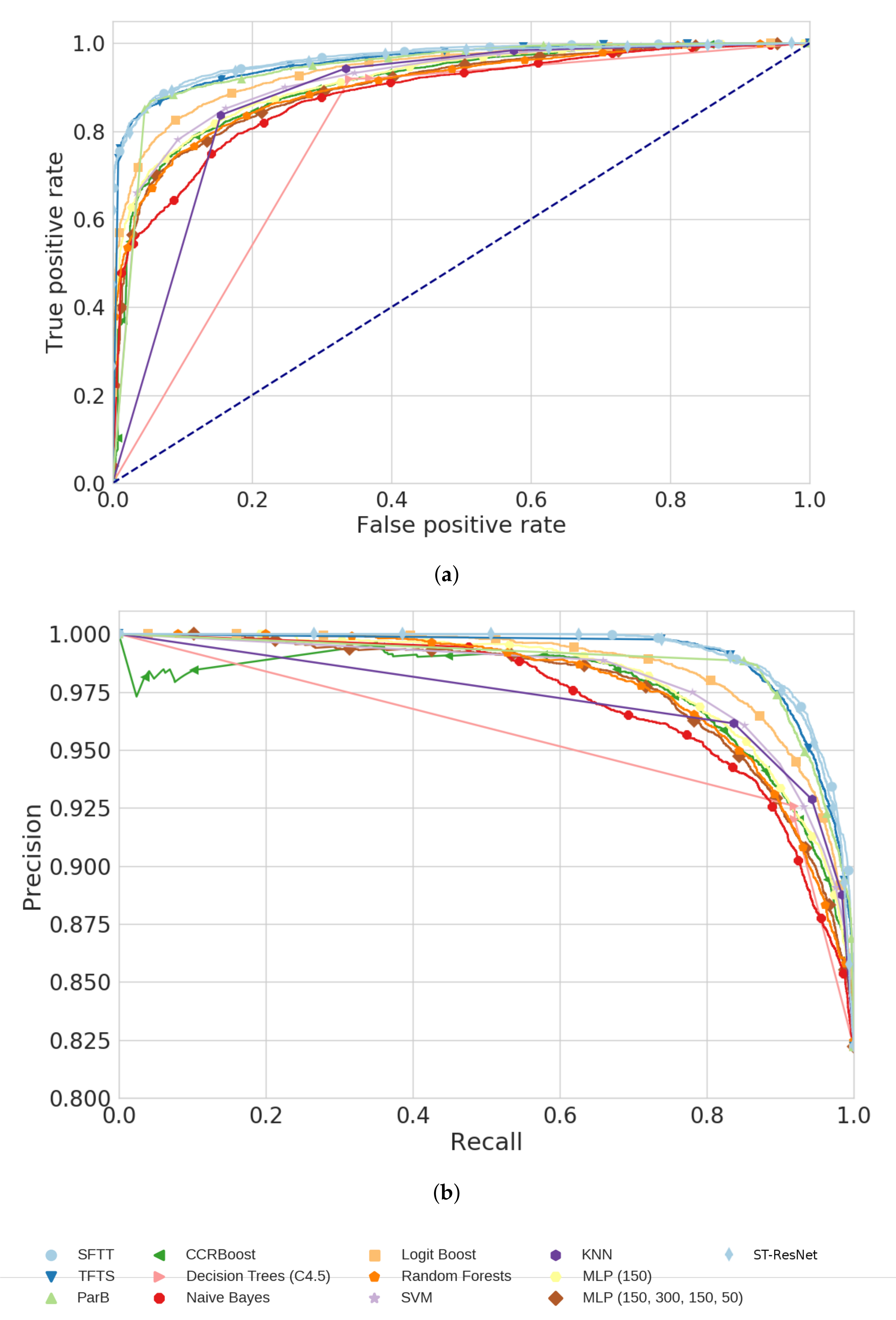
6.1. Evaluation of Models

By comparing the three main model building approaches, we investigate if the data are more correlated in the spatial or temporal axes. In the first approach, the spatial dimension of the data is explored before the detection of temporal structures (SFTT). For the second approach (TFTS), the temporal dimension is first explored and then, the temporal features are used to detect spatial features. In the third approach (i.e., ParB), we use two parallel branches, one to extract spatial features and one to extract temporal features. The two sets of features are then combined before they are given to the classifier. In Figure 4, we present the $F1score$, $AUCPR$, $AUROC$ and $PAI@5$, respectively for the DL approaches, compared to the 10 baseline approaches, per dataset for the “All Crimes” crime type in the highest resolution of $p=40$, i.e., $40\times 40$ cells. The ROC curves and PR curves for the same experiment are shown in Figure 5. Similar behaviour appears for the rest of the crime types.

From the results, we can see that all three DL approaches give consistently better performance than the baseline methods in the binary classification task of a cell being a hotspot or not, with SFTT being the winning approach. For each cell, the SFTT approach gives the highest scores in all metrics for all datasets except the San Francisco one. The TFTS approach follows in the second place while the ParB approach does not perform well in this task.

6.2. Evaluation of Cell Size

The second major parameter that we evaluated is the effect of spatial resolution on the approaches. The resolutions that were tested vary from the coarsest resolution of $p=16$ (i.e., $16\times 16$ cells grid) to the finest of $p=40$ cells grid with a step of $p=8$ cells and the results for every metric are presented in

Table 4. F1score, Precision-Recall AUC, ROC AUC and PAI@5 for different p (i.e., different resolutions) in the Philadelphia dataset for “All Crimes” crime type. The winning algorithm is in bold.

Algorithm	F1score				AUCPR				AUROC				PAI@5
	16	24	32	40	16	24	32	40	16	24	32	40	16	24	32	40
CCRBoost	0.93	0.92	0.88	0.88	0.99	0.99	0.98	0.97	0.92	0.92	0.90	0.91	1.87	1.94	1.86	2.00
Decision Trees (C4.5)	0.93	0.92	0.90	0.89	0.99	0.97	0.97	0.96	0.85	0.80	0.78	0.79	0.59	1.51	1.54	1.80
Naive Bayes	0.92	0.87	0.84	0.83	0.98	0.98	0.98	0.97	0.82	0.89	0.86	0.88	1.21	2.82	2.00	1.93
Logit Boost	0.94	0.92	0.91	0.89	1.00	0.99	0.99	0.99	0.99	0.96	0.94	0.94	0.81	1.73	2.52	1.91
SVM	0.94	0.93	0.91	0.90	0.99	0.99	0.98	0.98	0.91	0.93	0.90	0.90	0.06	0.12	0.19	0.25
Random Forests	0.94	0.92	0.90	0.89	1.00	0.99	0.98	0.98	0.97	0.94	0.91	0.92	1.04	2.44	1.93	1.98
KNN	0.94	0.92	0.91	0.89	0.99	0.98	0.97	0.97	0.86	0.87	0.84	0.88	0.93	1.66	1.89	2.29
MLP (150)	0.94	0.92	0.90	0.89	0.98	0.99	0.98	0.98	0.84	0.94	0.91	0.92	2.21	2.09	2.30	2.95
MLP (150, 300, 150, 50)	0.94	0.92	0.90	0.89	0.97	0.99	0.98	0.98	0.79	0.91	0.91	0.90	1.31	2.10	2.15	2.70
ST-ResNet	0.91	0.88	0.86	0.82	0.99	0.99	0.99	0.99	0.98	0.96	0.96	0.96	3.30	1.62	2.55	2.56
SFTT	0.99	0.97	0.96	0.94	1.00	1.00	1.00	0.99	0.99	0.98	0.97	0.97	4.02	4.34	4.14	4.33
TFTS	0.99	0.97	0.95	0.94	1.00	0.98	0.99	0.99	0.95	0.81	0.93	0.96	4.30	4.40	4.10	4.12
ParB	0.99	0.96	0.94	0.92	0.99	0.99	0.99	0.99	0.88	0.91	0.94	0.94	4.32	3.41	3.29	3.31

. While increasing the number of cells, the feature maps become sparser.

It is evident that increasing the spatial resolution leads to a deterioration of $F1score$ for all models, including the baselines. On the other hand, the $PAI$ metric seems to benefit from the greater detail in some of the compared algorithms, which is expected, since the same proportion of crimes is correctly predicted but inside a smaller proportion of the study area. In the AUC metrics, the SFTT approach constantly outperforms all other approaches.

Having these results as a guide to our further research, the SFTT approach was selected for the rest of our experiments as the winning configuration.

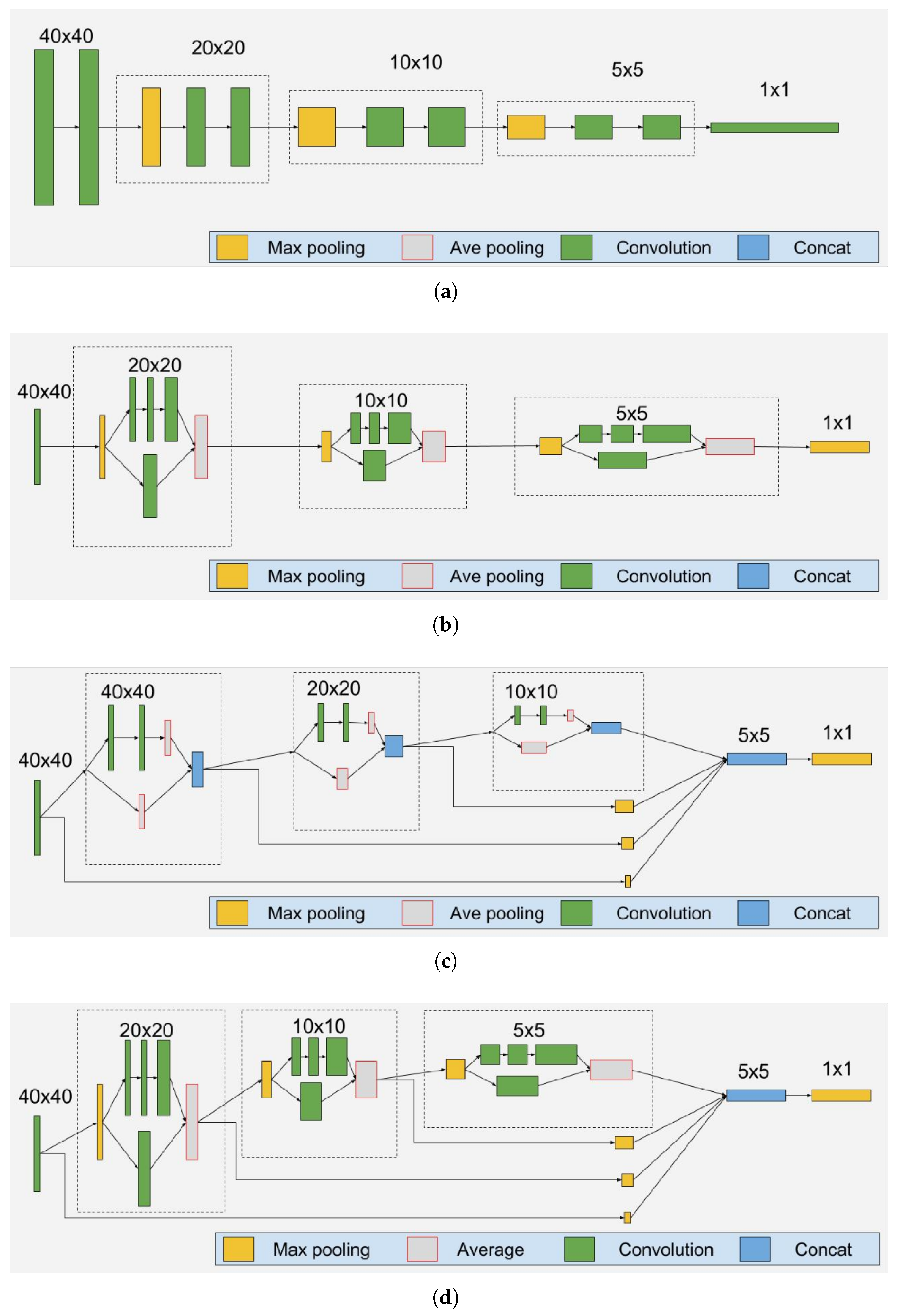
6.3. Evaluation of Spatial Body

Having selected the SFTT approach, Figure 6 presents a comparison of the 4 bodies’ performance for various crime types. In all of the metrics, the FastMask model has the worst performance compared to the other bodies. While the FastResMask body has similar performance with the ResNet body, the latter has fewer parameters (therefore a smaller memory footprint) and is faster to train (Table 1). We can conclude that for this task, the extraction of features from different scales of the data is redundant and ineffective.

The VGG body performs equivalently with the ResNet body in the F1score metric (Figure 6a) which measures the correctly identified hotspots when considering all the cells inside the study area. In the AUC metrics (Figure 6b,c), which measure the probability that a randomly selected hotspot is correctly identified as such, the VGG body performs better than the ResNet body.

On the other hand, in the 4 crime types with the more incidents, the performance of the VGG body is inferior to that of ResNet for the PAI metric (Figure 6d) which measures if the more significant (in terms of more occurring crimes) cells are marked as more probable to be hotspots.

A new set of experiments was conducted for the selection and modelling of input data with only 1 crime category as an input versus all 11 crime categories as input. Our experiments verified that the proposed setup of having all 11 crime categories as input channels contributes positively to the F1score performance of the model by a factor of $2.5\%$ in the Seattle dataset, up to $4.5\%$ in the Philadelphia dataset.

6.4. Evaluation of Temporal Body

The quality of temporal clues extracted from the temporal part of our SFTT model can be affected by the depth and the width of the RNN. To evaluate these two parameters we performed experiments firstly by changing only the depth of LSTM layers in the network and then by changing only the width of the LSTM layers.

The depth of the temporal part of the network is defined by the number of LSTM layers present in the network. For every consecutive LSTM layer, a new level of non-linear abstraction is introduced in the network. We evaluated the effect by using from one to nine LSTM layers to reveal that there was no significant gain by adding more layers. More specifically, the $F1score$ of our tested model in the Philadelphia “All Crimes”, which is the class with most data, was $0.94289\pm 0.00003$ in all examined depths. Following the same behaviour, the $F1score$ of the model on Philadelphia “Burglary” (sparse with few records) was at $0.76475\pm 0.00017$ for all numbers of LSTM layers.

The width of the network is defined by the number of hidden states that exist in each LSTM layer and defines the amount of temporal information that can be modelled. To examine the effect that LSTM layers’ width has on the performance of the model, we varied the width up to 500 hidden neurons in each LSTM layer. We observed in the results that almost all the available temporal information can be captured with LSTM layers of only 50 hidden neurons.

6.5. Evaluation of Batch Normalisation and Dropout

The amount of data that is available for the training process is fairly small, compared to image classification datasets with millions of samples. This lack of data can lead to networks that overfit by learning the training data but not being able to generalise properly.

In DL literature the two most common methods to overcome overfitting problems is the use of Batch Normalization and Dropout. We used Batch Normalization after every pooling layer and tested several variations of Dropout layers. When we removed Batch Normalization the performance dropped significantly.

A Dropout layer, randomly zeroes out a percentage of the input data values, during the training phase, thus creating variations of the training data in each epoch. These random variations effectively multiply the number of training samples and allow the networks to generalise better. By increasing the percentage of dropout, more virtual samples are created but the data become sparser. To find the best compromise, we investigated dropout percentages from 10% up to 90%. Adding more dropout helps the predictor to generalise a little bit better for the more populated “All Crimes” crime type in predicting the most probable hotspots. For all other crime types, varying the percentage of dropout has no measurable effect.

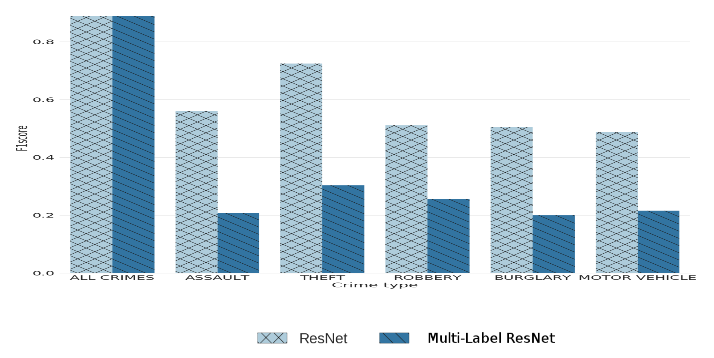
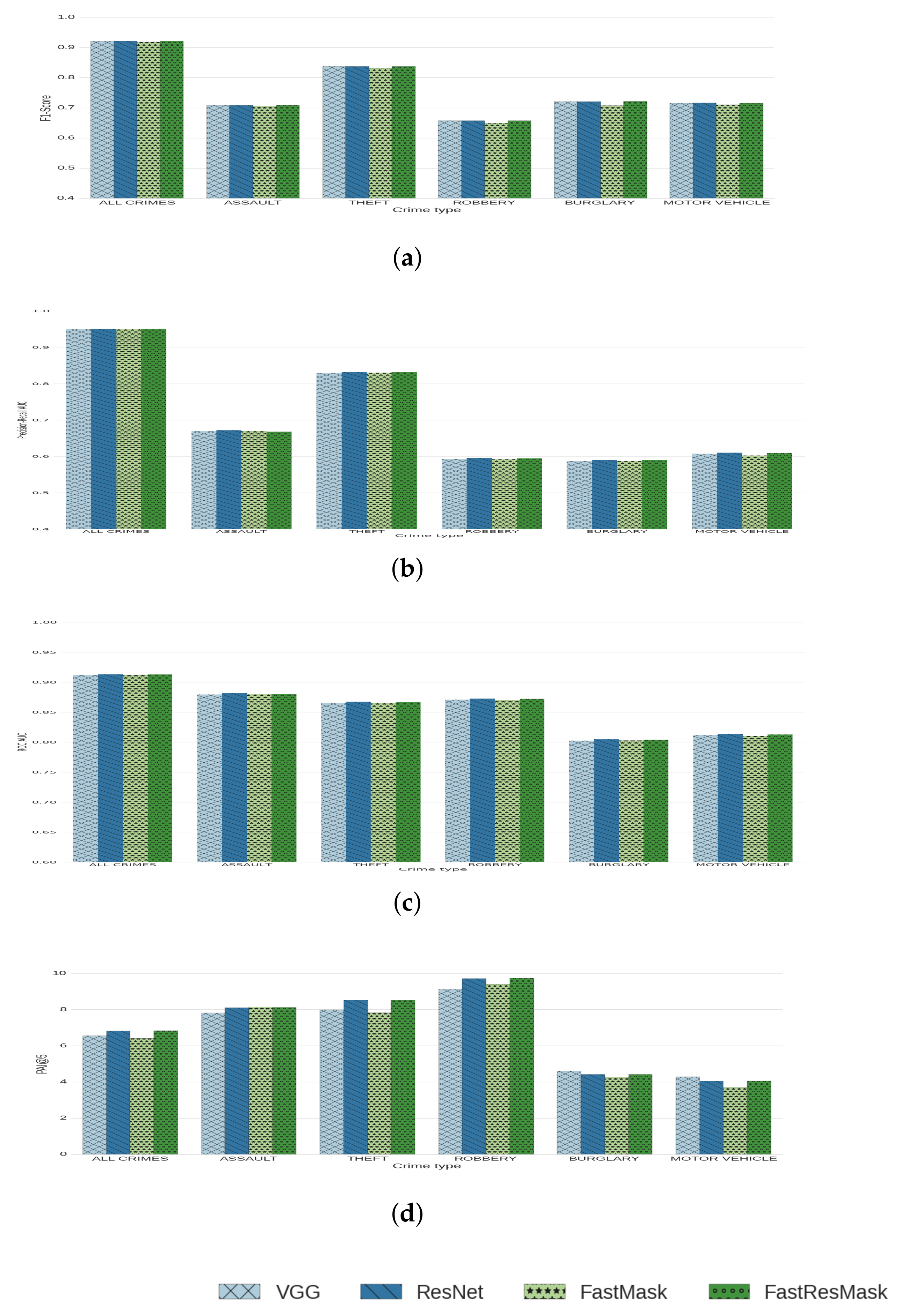
6.6. Multi-Label Hotspot Classification

As a final experiment on the configuration of the proposed approach, a multi-label classification was tested. The aim was to evaluate how the proposed model performs when simultaneously predicting the probability for each cell to be a hotspot for all possible crime types at the same time. To do so, the last layers’ dimension was changed from 1 (binary classification) to 11, which is the number of crime types in the dataset. The loss function was also modified from binary cross-entropy to multi-class cross-entropy. For the predictions of this setup to remain comparable with our previous results, we kept the last layer activation function to sigmoid, which is typical for the configuration of multi-label models. For this experiment, the SFTT model with ResNet spatial body was used and the results are presented in Figure 7. As is expected, the binary classification model outperforms the multi-label model in each crime type except the “All Crimes” type were the same performance is observed. This is observed due to class imbalance as well as the difficulty of the model to predict accurately all the labels (i.e., classes), due to the sparsity of the data.

7. Conclusions and Future Work

In this paper, we investigated the capability of DL methods to forecast hotspot areas in an urban environment, where crimes of certain types are more likely to occur in a defined future window. To achieve this goal we fed the DL methods with the minimum amount of data containing only spatial, temporal and crime type information. For the models to better predict the order of “hotness” we used a dual output setting where the second output is the number of crimes that occurred in the same future window. Moreover, we selected our SFTT model configuration as the winning one, compared it with 10 different algorithms in 5 crime incidence datasets and further analysed the selected parameters for robust results.

In the future, we will investigate if incorporating additional information into our systems, like temporal semantics, demographics, weather, street maps and points of interest in the area can help our model to learn better features. Temporal semantics can help the prediction of fluctuations in crime rates that depend on seasonal events, like holidays, and time of day events, like shift change in stores.

By replacing dense layers with convolution layers in both the temporal clues extraction and the classification parts of the model, in a full convolution network fashion, we can increase the spatial resolution. Another road that we did not explore is to pre-process and augment the available data. Preprocessing steps could include normalisation of the data and blind source separation, while data augmentation can come from flipping and rotating the data on their spatial dimensions. Additional data could be created by changing the shift of the temporal sliding window from daily to hourly rate.

References

1. Perry, W.L. Predictive Policing: The Role of Crime Forecasting in Law Enforcement Operations; Rand Corporation: Santa Monica, CA, USA, 2013. [Google Scholar]
2. Cohen, L.E.; Felson, M. Social change and crime rate trends: A routine activity approach. Am. Sociol. Rev. 1979, 44, 588–608. [Google Scholar] [CrossRef]
3. Cornish, D.B.; Clarke, R.V. The Reasoning Criminal: Rational Choice Perspectives on Offending; Transaction Publishers: Piscataway, NJ, USA, 2014. [Google Scholar]
4. Grubesic, T.H.; Mack, E.A. Spatio-temporal interaction of urban crime. J. Quant. Criminol. 2008, 24, 285–306. [Google Scholar] [CrossRef]
5. Johnson, S.D.; Bowers, K.; Hirschfield, A. New insights into the spatial and temporal distribution of repeat victimization. Br. J. Criminol. 1997, 37, 224–241. [Google Scholar] [CrossRef]
6. Johnson, S.D.; Bernasco, W.; Bowers, K.J.; Elffers, H.; Ratcliffe, J.; Rengert, G.; Townsley, M. Space–time patterns of risk: A cross national assessment of residential burglary victimization. J. Quant. Criminol. 2007, 23, 201–219. [Google Scholar] [CrossRef] [Green Version]
7. Bowers, K.J.; Johnson, S.D. Who commits near repeats? A test of the boost explanation. West. Criminol. Rev. 2004, 5, 12–24. [Google Scholar]
8. Breiman, L. Random forests. Mach. Learn. 2001, 45, 5–32. [Google Scholar] [CrossRef] [Green Version]
9. Zhang, H. The optimality of naive Bayes. AA 2004, 1, 3. [Google Scholar]
10. Cortes, C.; Vapnik, V. Support-vector networks. Mach. Learn. 1995, 20, 273–297. [Google Scholar] [CrossRef]
11. Wang, B.; Zhang, D.; Zhang, D.; Brantingham, P.J.; Bertozzi, A.L. Deep Learning for Real Time Crime Forecasting. arXiv 2017, arXiv:1707.03340. [Google Scholar]
12. Levine, N.; CrimeStat, I. A Spatial Statistics Program for the Analysis of Crime Incident Locations; Ned Levine and Associates: Houston, TX, USA; The National Institute of Justice: Washington, DC, USA, 2002.
13. Williamson, D.; McLafferty, S.; McGuire, P.; Ross, T.; Mollenkopf, J.; Goldsmith, V.; Quinn, S. Tools in the Spatial Analysis of Crime. Mapping and Analysing Crime Data; Hirschfield, A., Bowers, K., Eds.; Taylor & Francis: London, UK; New York, NY, USA, 2001; Volume 1, p. 187. [Google Scholar]
14. Rosenblatt, M.; Lii, K.S.; Politis, D.N. Remarks on some nonparametric estimates of a density function. Ann. Math. Stat. 1956, 27, 832–837. [Google Scholar] [CrossRef]
15. Chainey, S.; Tompson, L.; Uhlig, S. The utility of hotspot mapping for predicting spatial patterns of crime. Secur. J. 2008, 21, 4–28. [Google Scholar] [CrossRef]
16. Eck, J.; Chainey, S.; Cameron, J.; Wilson, R. Mapping Crime: Understanding Hotspots; U.S. Department of Justice Office of Justice Programs: Washington, DC, USA, 2005. Available online: https://discovery.ucl.ac.uk/id/eprint/11291/1/11291.pdf (accessed on 12 June 2019).
17. Chainey, S.; Ratcliffe, J. GIS and Crime Mapping; John Wiley & Sons: Hoboken, NJ, USA, 2013. [Google Scholar]
18. Bishop, C.M. Pattern recognition. Mach. Learn. 2006, 128, 1–58. [Google Scholar]
19. Silverman, B.W. Density Estimation for Statistics and Data Analysis; CRC Press: Boca Raton, FL, USA, 1986; Volume 26. [Google Scholar]
20. de Queiroz Neto, J.F.; dos Santos, E.M.; Vidal, C.A. MSKDE-Using Marching Squares to Quickly Make High Quality Crime Hotspot Maps. In Proceedings of the 2016 29th SIBGRAPI Conference on Graphics, Patterns and Images (SIBGRAPI), Sao Paulo, Brazil, 4–7 October 2016; pp. 305–312. [Google Scholar]
21. Mohler, G.O.; Short, M.B.; Brantingham, P.J.; Schoenberg, F.P.; Tita, G.E. Self-exciting point process modeling of crime. J. Am. Stat. Assoc. 2011, 106, 100–108. [Google Scholar] [CrossRef]
22. Ratcliffe, J.H. A temporal constraint theory to explain opportunity-based spatial offending patterns. J. Res. Crime Delinq. 2006, 43, 261–291. [Google Scholar] [CrossRef]
23. Ghazvini, A.; Abdullah, S.N.H.S.; Kamrul Hasan, M.; Bin Kasim, D.Z.A. Crime Spatiotemporal Prediction with Fused Objective Function in Time Delay Neural Network. IEEE Access 2020, 8, 115167–115183. [Google Scholar] [CrossRef]
24. Nakaya, T.; Yano, K. Visualising Crime Clusters in a Space-time Cube: An Exploratory Data-analysis Approach Using Space-time Kernel Density Estimation and Scan Statistics. Trans. GIS 2010, 14, 223–239. [Google Scholar] [CrossRef]
25. Toole, J.L.; Eagle, N.; Plotkin, J.B. Spatiotemporal correlations in criminal offense records. ACM Trans. Intell. Syst. Technol. (TIST) 2011, 2, 38. [Google Scholar] [CrossRef]
26. Olligschlaeger, A.M. Artificial neural networks and crime mapping. Crime Mapp. Crime Prev. 1997, 1, 313–348. [Google Scholar]
27. Kianmehr, K.; Alhajj, R. Effectiveness of support vector machine for crime hot-spots prediction. Appl. Artif. Intell. 2008, 22, 433–458. [Google Scholar] [CrossRef]
28. Yu, C.H.; Ward, M.W.; Morabito, M.; Ding, W. Crime forecasting using data mining techniques. In Proceedings of the 2011 IEEE 11th International Conference on Data Mining Workshops, Vancouver, BC, Canada, 11 December 2011; pp. 779–786. [Google Scholar]
29. Gorr, W.; Olligschlaeger, A.; Thompson, Y. Short-term forecasting of crime. Int. J. Forecast. 2003, 19, 579–594. [Google Scholar] [CrossRef]
30. Feng, M.; Zheng, J.; Ren, J.; Hussain, A.; Li, X.; Xi, Y.; Liu, Q. Big Data Analytics and Mining for Effective Visualization and Trends Forecasting of Crime Data. IEEE Access 2019, 7, 106111–106123. [Google Scholar] [CrossRef]
31. Eftelioglu, E.; Shekhar, S.; Kang, J.M.; Farah, C.C. Ring-Shaped Hotspot Detection. IEEE Trans. Knowl. Data Eng. 2016, 28, 3367–3381. [Google Scholar] [CrossRef]
32. Xu, J.; Tan, P.N.; Zhou, J.; Luo, L. Online Multi-Task Learning Framework for Ensemble Forecasting. IEEE Trans. Knowl. Data Eng. 2017, 29, 1268–1280. [Google Scholar] [CrossRef]
33. Yu, C.H.; Ding, W.; Morabito, M.; Chen, P. Hierarchical Spatio-Temporal Pattern Discovery and Predictive Modeling. IEEE Trans. Knowl. Data Eng. 2016, 28, 979–993. [Google Scholar] [CrossRef]
34. He, K.; Zhang, X.; Ren, S.; Sun, J. Deep residual learning for image recognition. In Proceedings of the IEEE Conference on Computer Vision and Pattern Recognition, Las Vegas, NV, USA, 27–30 June 2016; pp. 770–778. [Google Scholar]
35. Simonyan, K.; Zisserman, A. Two-stream convolutional networks for action recognition in videos. Adv. Neural Inf. Process. Syst. arXiv 2014, arXiv:1406.2199. [Google Scholar]
36. Wu, Z.; Wang, X.; Jiang, Y.G.; Ye, H.; Xue, X. Modeling spatial-temporal clues in a hybrid deep learning framework for video classification. In Proceedings of the 23rd ACM international conference on Multimedia, Brisbane, Australia, 26–30 October 2015; ACM: New York, NY, USA, 2015; pp. 461–470. [Google Scholar]
37. Hochreiter, S.; Schmidhuber, J. Long short-term memory. Neural Comput. 1997, 9, 1735–1780. [Google Scholar] [CrossRef]
38. Ruta, D.; Gabrys, B.; Lemke, C. A generic multilevel architecture for time series prediction. IEEE Trans. Knowl. Data Eng. 2011, 23, 350–359. [Google Scholar] [CrossRef]
39. Simonyan, K.; Zisserman, A. Very deep convolutional networks for large-scale image recognition. arXiv 2014, arXiv:1409.1556. [Google Scholar]
40. Hu, H.; Lan, S.; Jiang, Y.; Cao, Z.; Sha, F. FastMask: Segment Multi-scale Object Candidates in One Shot. arXiv 2016, arXiv:1612.08843. [Google Scholar]
41. Russakovsky, O.; Deng, J.; Su, H.; Krause, J.; Satheesh, S.; Ma, S.; Huang, Z.; Karpathy, A.; Khosla, A.; Bernstein, M.; et al. Imagenet large scale visual recognition challenge. Int. J. Comput. Vis. 2015, 115, 211–252. [Google Scholar] [CrossRef] [Green Version]
42. Quinlan, J.R. C4. 5: Programs for Machine Learning; Elsevier: Amsterdam, The Netherlands, 2014. [Google Scholar]
43. Friedman, J.; Hastie, T.; Tibshirani, R. Additive logistic regression: A statistical view of boosting (with discussion and a rejoinder by the authors). Ann. Stat. 2000, 28, 337–407. [Google Scholar] [CrossRef]
44. Arya, S.; Mount, D.M.; Netanyahu, N.S.; Silverman, R.; Wu, A.Y. An optimal algorithm for approximate nearest neighbor searching fixed dimensions. J. ACM (JACM) 1998, 45, 891–923. [Google Scholar] [CrossRef] [Green Version]
45. Ruck, D.W.; Rogers, S.K.; Kabrisky, M.; Oxley, M.E.; Suter, B.W. The multilayer perceptron as an approximation to a Bayes optimal discriminant function. IEEE Trans. Neural Netw. 1990, 1, 296–298. [Google Scholar] [CrossRef]
46. Zhang, J.; Zheng, Y.; Qi, D. Deep Spatio-Temporal Residual Networks for Citywide Crowd Flows Prediction. In Proceedings of the Thirty-first AAAI Conference on Artificial Intelligence, San Francisco, CA, USA, 4–9 February 2017; pp. 1655–1661. [Google Scholar]
47. Pedregosa, F.; Varoquaux, G.; Gramfort, A.; Michel, V.; Thirion, B.; Grisel, O.; Blondel, M.; Prettenhofer, P.; Weiss, R.; Dubourg, V.; et al. Scikit-learn: Machine learning in Python. J. Mach. Learn. Res. 2011, 12, 2825–2830. [Google Scholar]
48. Chollet, F. Keras. 2015. Available online: https://github.com/keras-team/keras (accessed on 20 February 2017).
49. Abadi, M.; Agarwal, A.; Barham, P.; Brevdo, E.; Chen, Z.; Citro, C.; Corrado, G.S.; Davis, A.; Dean, J.; Devin, M.; et al. TensorFlow: Large-Scale Machine Learning on Heterogeneous Systems. 2015. Available online: tensorflow.org (accessed on 20 July 2017).
50. NVIDIA CUDA Programming Guide NVIDIA. 2010. Available online: http://developer.download.nvidia.com (accessed on 24 April 2018).
51. Fawcett, T. An introduction to ROC analysis. Pattern Recognit. Lett. 2006, 27, 861–874. [Google Scholar] [CrossRef]
Figure 1. Overview of the sequence of feature extraction: (a) the spatial features first then the temporal (SFTT), (b) the temporal features first then the spatial (TFTS) and (c) spatial and temporal features in two parallel branches (ParB).
Forecasting 03 00046 g001
Figure 2. Convolutional network body architectures used for the extraction of spatial information: (a) VGGNet, (b) ResNet, (c) FastMask and (d) FastResidualMask. Convolutional layers are coloured green, pooling layers are coloured yellow and the grey are non-parametric layers (i.e., concatenation).
Forecasting 03 00046 g002
Figure 3. Philadelphia map overlayed with a plotting of all incidents that occurred in 2006.
Forecasting 03 00046 g003
Figure 4. (a) F1score, (b) PR AUC, (c) ROC AUC and (d) PAI@5 per dataset for “All Crimes” crime type for the 3 DL models and 10 baseline approaches for a cell size of 450 m (40 by 40). Best viewed in colour.
Forecasting 03 00046 g004
Figure 5. (a) ROC Curves and (b) Precision-Recall Curves for “All Crimes” crime type for the 4 DL bodies and 10 baseline approaches in the Philadelphia dataset. Best viewed in colour.
Forecasting 03 00046 g005
Figure 6. (a) F1score, (b) PR AUC, (c) ROC AUC and (d) PAI@5 per crime type in the Philadelphia dataset, for 4 spatial clue extractor bodies. Best viewed in colour.
Forecasting 03 00046 g006
Figure 7. F1score per crime type in the Philadelphia dataset, for binary and multi-label hotspot prediction. Best viewed in colour.
Forecasting 03 00046 g007