Article

Modeling of Lake Malombe Annual Fish Landings and Catch per Unit Effort (CPUE)

by
Rodgers Makwinja
1,2,*,
Seyoum Mengistou
1,
Emmanuel Kaunda
3,
Tena Alemiew
4,
Titus Bandulo Phiri
2,
Ishmael Bobby Mphangwe Kosamu
5 and
Chikumbusko Chiziwa Kaonga
5
1
African Centre of Excellence for Water Management, Addis Ababa University, P.O. Box 1176, Addis Ababa, Ethiopia
2
Senga Bay Fisheries Research Centre, P.O. Box 316, Salima, Malawi
3
African Centre of Excellence in Aquaculture and Fisheries (AquaFish), Lilongwe University of Agriculture and Natural Resources, P.O. Box 219, Lilongwe, Malawi
4
Water and Land Resource Centre of Addis Ababa University, P.O. Box 3880, Addis Ababa, Ethiopia
5
Physics and Biochemical Sciences Department, The Malawi Polytechnic, University of Malawi, P/Bag 303, P.O. Box 537, Chichiri, Blantyre, Malawi
*
Author to whom correspondence should be addressed.
Forecasting 2021, 3(1), 39-55; https://doi.org/10.3390/forecast3010004
Submission received: 24 October 2020 / Revised: 26 January 2021 / Accepted: 26 January 2021 / Published: 8 February 2021
(This article belongs to the Section Environmental Forecasting)

Abstract

:
Forecasting, using time series data, has become the most relevant and effective tool for fisheries stock assessment. Autoregressive integrated moving average (ARIMA) modeling has been commonly used to predict the general trend for fish landings with increased reliability and precision. In this paper, ARIMA models were applied to predict Lake Malombe annual fish landings and catch per unit effort (CPUE). The annual fish landings and CPUE trends were first observed and both were non-stationary. The first-order differencing was applied to transform the non-stationary data into stationary. Autocorrelation functions (AC), partial autocorrelation function (PAC), Akaike information criterion (AIC), Bayesian information criterion (BIC), square root of the mean square error (RMSE), the mean absolute error (MAE), percentage standard error of prediction (SEP), average relative variance (ARV), Gaussian maximum likelihood estimation (GMLE) algorithm, efficiency coefficient (E2), coefficient of determination (R2), and persistent index (PI) were estimated, which led to the identification and construction of ARIMA models, suitable in explaining the time series and forecasting. According to the measures of forecasting accuracy, the best forecasting models for fish landings and CPUE were ARIMA (0,1,1) and ARIMA (0,1,0). These models had the lowest values AIC, BIC, RMSE, MAE, SEP, ARV. The models further displayed the highest values of GMLE, PI, R2, and E2. The “auto. arima ()” command in R version 3.6.3 further displayed ARIMA (0,1,1) and ARIMA (0,1,0) as the best. The selected models satisfactorily forecasted the fish landings of 2725.243 metric tons and CPUE of 0.097 kg/h by 2024.

1. Introduction

Lake Malombe is located within the Upper and Middle Shire River basin in the Southern part of Malawi. The lake is one of the most important freshwater ecosystems in terms of providing fishing resources in Malawi [1]. It is mostly dominated by Cichlidae, Claridae, and Cyprinidae families though other genera such as Bathyclarias, Fossorochromis, Pseudotropheus, Caprichromis, and Brycinus are also equally important. Historically, Lake Malombe is well known for massive fisheries resource depletion in Africa since the 1960s [2]. The relative biomass index of the lake fishery decreased from 1.01 units in the 1970s to 0.3 units in 2016. Fish biomass landings also decreased from 44,000 metric tons in 1981 to 6000 in 2018. The above evidence impelled the Malawi government to take a command control approach (stipulated in the guideline of Fisheries Act [3] formulated based on the Laws of Malawi, Chapter 66:05 1974 and amended in 1976, 1977, 1979, 1984, 1996, and 1997, which include gear licensing, gear and mesh size regulations, implementation of the closed season, banning of fine-meshed beach seines and regulating fishing effort) to reverse the situation. However, this approach faced strong resistance in its implementation and hence failed to achieve its objective. In the 1980s, the fisheries co-management approach was introduced [4]. This approach was considered to be more holistic and assumed that Lake Malombe fishing communities affected by the collapse of the fishery had the potential to find a sustainable solution to address the impact through collaborative planning. The approach was further introduced in response to the perceived failure of the command control management approach in preventing the decline of fish stocks in the lake and the lack of proper government resources to effectively manage the fisheries. However, several researchers, fisheries experts, and experienced fishers argued that the co-management approach in Lake Malombe was also a failure. Hara [5] in his study noted that lack of information on social, cultural, and institutional factors underlying the exploitation patterns of lake fishery was the main reason for the failure of the co-management approach in Lake Malombe. It was further argued that the implementation arrangements of this approach also followed the top-down method, was donor-driven, not formed within a new institutional vacuum, and did not take into account the institutional landscape and diversity that impacted the functioning and performance of the structures [6].
The failure of fisheries co-management prompted the Malawi government to develop an ecosystem-based fisheries management approach. The forecasting of total annual biomass landings and catch per unit effort (CPUE) is a basic component embedded in this approach to effectively manage the stocks. For example, one of the main objectives of this new approach is to set a practical fishing effort in a concrete area during the known breeding period for stock replacement. To achieve this objective, it is necessary to predict uncontrollable biomass trends and possible abundance of the stock biomass in the lake—an approach that requires the development and the application of stock production conceptual models. These models are very relevant since they are directly linked to the concept of the precautionary approach—a basic concept in fish stock management [7]. Schaeffer and Fox production models, also known as surplus production models (a model associated with maximum sustainable yield (MSY)), have already been commonly applied to depict the status of fishery in Lake Malawi and other inland lakes. Although these models are acceptable in fishery management, their applications are still questionable. For example, the models only depict the current picture of the fishery using time-series trends and lack the power of prediction. Other models such as state-space [8] and Bayesian [8] have also been applied with little success. The time-series approach, however, has been indispensable in understanding natural resources systems and the development of better management policies. It is described as the best approach to fisheries modeling and stock assessment. It provides a feasible way to examine the time series data and provide a prediction of the catches. The approach demands fewer biological assumptions than other traditional fisheries models and with simple mathematical techniques and few assumptions, it can significantly reduce the modeling costs including research costs. Several researchers have recommended the time series approach in fisheries stock assessment. For example, Stergiou [9] highly recommended a time series approach and efficiently predicted the Mullidae fishery in the Eastern Mediterranean Sea. Selvaraj et al. [10] successfully developed autoregressive integrated moving average (ARIMA) models to predict fishery landings in the Colombian Pacific Ocean. Koutroumanidis et al. [11], however, combined ARIMA models and fuzzy expected intervals software to forecast fishery landings in Thessaloniki, Greece. Researchers such as Park [12], Georgakarakos et al. [13], Lioret et al. [14], Prista et al. [15], Raman et al. [16], and Stergiou [17] also preferred time series modeling in their predictions of the marine fishery, understanding the dynamics of the fishery, monitoring and forecasting fish landings in data-scarce regions. This study used ARIMA (p,d,q) models to forecast Lake Malombe fish landings and CPUE.

2. Materials and Methods

2.1. The Study Area

Lake Malombe (Figure 1) is located in the Shire River Basin (the largest and longest river basin in Malawi and fourth-largest in Africa). The Shire River basin lies in the southern part of the East Africa Great Rift valley system.
It originates from Lake Malawi at Samama and flows 400 km south and southeast to its confluence with the Zambezi River at Ziu Ziu in Mozambique with an estimated catchment area of 18,945 km2 divided into the upper, middle, and lower sections. The upper section of the Shire River Basin (with a total channel bed drop of about 15 m over a distance of 130 km) lies between Mangochi and Machinga districts. From Mangochi, the Upper Shire River Basin drains into Lake Malombe (coordinates 14°40′0″ S 35°15′0″ E) 8 km south of Mangochi and continues to flow through swampy banks flanked by hills and escarpment. Lake Malombe is documented as the third-largest in Malawi with an estimated total area of 162 square miles (420 km2), length of 30 km, a width of 17 km, and water depth not exceeding 6 m [18]. The communities around the lake catchment are predominately fishers [19]. The lake has approximately 65 fishing beaches scattered over the three major administrative strata known as Lake Malombe East coded as 1.1, Lake Malombe West coded 1.2, and Upper Shire coded 1.3 [19]. The surrounding area of Lake Malombe is densely populated by the Yao ethnic tribe consisting of over 85% [19] of the fishing population. Few tribes such as Chewa, Lhomwe, and Nyanja are also found around the Lake.

2.2. Data Sources

2.2.1. Fish Biomass

Department of Fisheries through its statistical office under the Malawi Fisheries Management Act (1997) is mandated to collect fish landing data on a weekly basis from artisanal fishermen. In Lake Malombe, the fish landing data is collected using Malawi Traditional Fishery (MTF)—a computerized gear-based sampling technique. The mathematical model below is used to determine the fish landings:
B = c t ¯ . A a . x i
where c t ¯ is the mean catch per unit effort obtained per administrative stratum during the survey, A is the total area of the stratum and a is the area swept by the net during the unit effort and x i being a proportion of the fish in the path of the gear that is returned by a net. The data is entered into the catch and effort statistics database hosted by Monkey Bay Fisheries Research Division of the Department of Fisheries. Therefore, the 43 years’ annual fish landings data used in this study was the summation of annual fish landings from different species in all Lake Malombe strata expressed in metric tons.

2.2.2. The Estimation of Catch per Unit Effort (CPUE)

The catch per unit effort (CPUE) data is collected alongside fish biomass landings. It is defined as an estimate of stock size [20]. It shows if the relationship between catch and effort is linear through the origin. Traditionally, there are two ways to calculate CPUE:
CPUE 1 = C i f i n = C f ¯
CPUE 2 = C i f i = C ¯ f ¯
where C i is defined as the ith catch (usually expressed in weight) and f i is its respective fishing effort [21]. Griffiths [22] named CPUE 1 as a weighted index of density and CPUE 2 as the unweighted index of density reasoning that the ratio CPUE 2 CPUE 1 , which he called the index of concentration, would exceed unity in areas of higher-than-average density. If fishing is at random, the index of concentration is 1 and if fishing effort is applied in those areas with less than average density, the ratio is less than 1. Another ratio estimator, that does not have much intuition, is presented by Snedecor and Cochran [23] (Equation (4)):
CPUE 3 = C i . f i f i 2 = C . f ¯ f 2
where C is proportional to f, the regression line between them statistically goes through the origin and can be fitted by a simple model C i = β f i + ε i . The above three equations are unbiased estimates of the population ratio β in normally distributed populations. The choice among the three is a matter of precision.

2.2.3. Conceptual Framework of the ARIMA Model

This paper presents Box and Jerkins approaches that were followed to model and forecast time series data using autoregressive integrated moving average (ARIMA) models. To model the fish landings and CPUE data, the traditional statistical models such as autoregressive (AR), smoothing, moving average (MA) and autoregressive integrated moving average (ARIMA) were applied. The autoregressive (AR (p)) model is expressed as
Y t = α 1 γ t 1 + α 2 γ t 2 + + α p γ t p + ε t
where Y t is the dependent variable γ at time t, γ t 1 + γ t 2 + + γ t p are the lagged dependent variables while α 1 + α 2 + + α p are the unknown parameters of the model α 1 0 and ε t is the value of the disorders term at time t, i, i.d. ε t ~ 0 , α 2 : p-the number of lagged values of y and represent the order of the process. The moving average (MA (q)) is defined by a function of its present and q-past disorders (lagged error) and is expressed as
Y t = ε t + β 1 ε t 1 + β 2 ε t 2 + + β q ε t q
where Y t is the dependent variable y at time t, ε t 1 , ε t 2 ε t q means lagged disturbances, and β 1 , β 2 . β q means unknown parameters of the model β q 0 , ε t ~ N 0 , α 2 q the number of lagged values of y and represents the order of the process. The two-process (AR) and (MA) are combined to form the autoregressive moving average model (ARMA (p,q)) expressed as:
Y t = α 1 γ t 1 + α 2 γ t 2 + + α p γ t p + ε t + β 2 ε t 2 + β q ε t q
However, the ARMA model works with stationary data which is not the case with fish landings and CPUE data [24]. Therefore, the application of differencing to remove a mean trend from non-stationary series is the common procedure for transforming non-stationary data to stationary [25]. The procedure has been advocated in the Box–Jenkins approach [26]. In this paper, the autoregressive integrated moving average model (ARIMA (p,d,q)) is introduced to deal with non-stationary data. The general form of the ARIMA model is
α L Δ d γ t = β L ε t   with   Δ 0 = 1   and   α L Δ d γ t
where a new time series is obtained by differencing the initial series γ t d . In the fisheries context, p describes the movements of the data series, d represents the degree of difference used to achieve stationarity and q represents the smoothing technique used to estimate secular trends. The autocorrelation (AC) and partial autocorrelation (PAC) functions are used to extract the periodic component of the time series and construct ARIMA models suitable for explaining time series data. The ACF is defined as the sequence of values:
τ t = C t C 0   T = 0 ,   1 T     1
where
C T = 1 T t = τ T 1 γ t γ ¯ γ t τ γ ¯
is the empirical autocovariance at lag τ and C o is the sample variance. The ACF reveals regular moving average spikes. For example, if the model has an MA (1) component, then there will only be one regular significant spike. If the model has an MA (2) component, then the model will have two regular spikes. The sample ACF ρ τ at lag, τ is simply the correlation between two sets of residuals obtained from regressing the elements γ t and γ t   τ + 1 on the set of intervening values. The PAC reveals a spike at the lag of the interaction term. Different combinations of multiplicative parameters were estimated to determine whether the identified parameters were statistically significant.
To evaluate the adequacy and performance of the models during the validation process, a series of measures of accuracy were applied. The correlation coefficient (R) was used to depict the relationship between observed and predicted fish landings and CPUE. On the other hand, the coefficient of determination (R2) described the proportion of the total variance applied and was explained by the model. Other significant measures of variance such as standard error of prediction (SEP), the coefficient of efficiency (E2), and the average relative variance (ARV) were also applied to see how far the model was able to explain the total variance of the data. It was further noted that there was a need to quantify the errors in the same series of variables and these errors include the square root of the mean square error (RMSE) and the mean absolute error (MAE) expressed as:
RMSE = i = 1 N Q T Q ^ T 2 N = MSE
MAE = i = 1 N Q t Q ^ t N
where Q t is the observed total annual fish landings or CPUE at the time t, Q ^ t is the estimated total annual fish landings or CPUE at time t, and N is the total number of observations of the validation set. The percent standard error of prediction (SEP) was expressed as
SEP = 100 Q ¯ t RMSE
where Q ¯ is the mean observed total annual biomass or CPUE of the validation set. The coefficient of efficiency E 2 and the average relative variance (ARV) were expressed as:
E 2 = 1 i = 1 N Q t Q ^ t 2 i = 1 N Q t Q ¯ t 2
ARV = i = 1 N Q t Q ^ t 2 i = 1 N Q t Q ¯ t 2 1 E 2
The sensitivity to outliers due to the squaring of the different terms is linked to E 2 or equivalent to ARV. A value of zero for E 2 suggests that the observed average Q ^ is as good as a predictor of the model, while negative values indicate that the observed average is a better predictor than the model. For the perfect match, the values of R 2 and E 2 should be close to one and those of SEP and ARV close to zero. The persistence index (PI) was also used for the model performance evaluation.
P I = 1 i = 1 N Q t Q ^ t 2 i = 1 N Q t Q t L 2
where Q t L is the observed fishery landings or CPUE at the time step t L and L is the lead-time. The PI values of one reflect a perfect adjustment between predicted and the observed values and a value of zero indicates that the model is not suitable. Negative PI means that the model is degrading the original trend meaning that it has the worst performance. The t ratios of the parameters to their standard error were also estimated. The Ljung–Box Chi-squared test was used to estimate whether the overall correlogram of the residuals displayed any methodical error. The Ljung–Box Chi-squared test is expressed as
Q = n n + 2 n k 1 r k 2
where rk (k = 1……… m) are residual AC and n is the number of observations used to fit the model. Akaike information criterion (AIC) and Bayesian information criterion (BIC) was calculated to give the possibility to compare with values obtained from other models. The AIC is expressed as
A I C = 2 ln f y + 2 k
where 2 ln f y means the goodness of fit while +2k means model complexity and k is the number of model parameters. Note, the model with the smallest AIC is chosen as the finest. The BIC was calculated as:
BIC = log MSE + m log N N
The Gaussian maximum likelihood estimation (GMLE) algorithm was further used to check the model adequacy. The GMLE was expressed by firstly denoting the elements of τ 1   and   τ 2 in ascending order as
j 1 < j 2 < < j p   a n d   i 1 < i 2 < < i q
Let θ 1 , , θ p + q T = b j i , , b j p , . , b j p , σ i 1 . , σ i q T , assuming = Θ ,   where   Θ R p + q is the parameter space. Given the parameter ,   Θ is a compact set containing the true value θ o as an interior point and observation X u , v , u = 1 , . , N 1 , v = 1 , , N 2 , the GMLE function was expressed as
L θ 2 σ N θ 1 2 exp 1 2 σ 2 X T θ 1 X
where N = N 1 N 2 , X is an N.1 vector consisting of N observation in ascending order and
θ = 1 2 σ 2 v a r X
is independent of σ 2 . The GMLE estimators were expressed as
θ ^ = a r g m i n log X T θ 1 X / N + θ Θ N 1 log [ θ ] , θ ^ 2 = X T θ ^ 1   X / N
Once the suitable time series model estimated its unknown parameters and established that the model fits well, the next step was to forecast fishery landings and CPUE values. In this context, the autoregressive model is represented as follows:
Y t = u = 1 π μ γ t μ + ε t
The next observation beyond y1…………yT is predicted using the model expressed below
Y ^ t + 1 = u = 1 π ^ μ γ t + 1 μ
where the π ^ μ are obtained by substituting the estimated parameters in the theoretical ones. The forecast γ t + 1 is obtained and used to forecast γ t + 2 which later is used to generate γ t + 3 . The process is used to obtain a forecast out of any point in the future.

3. Results

Modeling and forecasting of fish landings and CPUE were conducted based on the raw data. The precision and characteristics of ARIMA models were studied in detail following the Box–Jenkins approach. The model parameters were identified, estimated, and verified. The model shown in Figure 2 is based on the 43 years’ time-series data from 1976 to 2019.
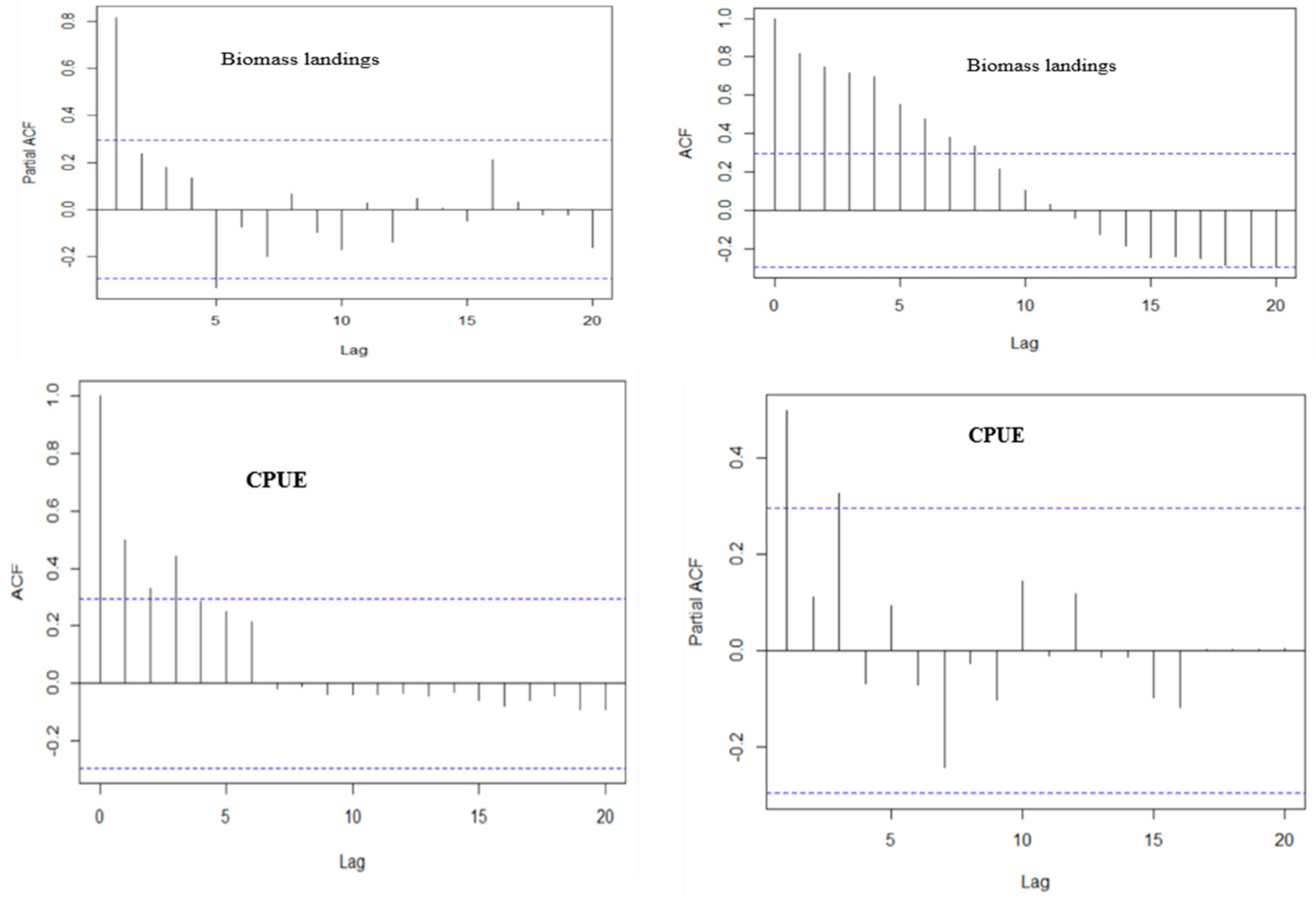
The first approach to ARIMA modeling was data inspection. Figure 2 shows that the fishery landing trend was very unstable with the highest observed from 1980 to 1990. The same observation is made in the catch per unit effort (CPUE) data plot which shows the highest within the period from 1976 to 1980. Figure 3 on the other hand shows the autocorrelation (AC) and partial autocorrelation (PAC) functions of the original fish landings time series data.
The AC is significantly higher than zero and gradually decreases to a zero function of the number of lags demonstrating that the time series data were not stationary. Similar results were observed in CPUE data series.

3.1. Model Identification

From the time series plot (above), it was very apparent that the time series data for fishery landings and CPUE had a random walk behavior and therefore had to be differenced. Differencing is an explicit option in ARIMA modeling [27]. It is implicitly a part of random walk and exponential smoothing models. In this paper, the first-order differencing was applied and the results were inspected in the form of the data plot. Figure 4 shows that time-series data of the first-order difference was stationary in mean and variance and therefore, it was suggested that an ARIMA (p,1,q) model was probably the best. The selected model was able to remove the trend component of the time series to remain with irregular components.
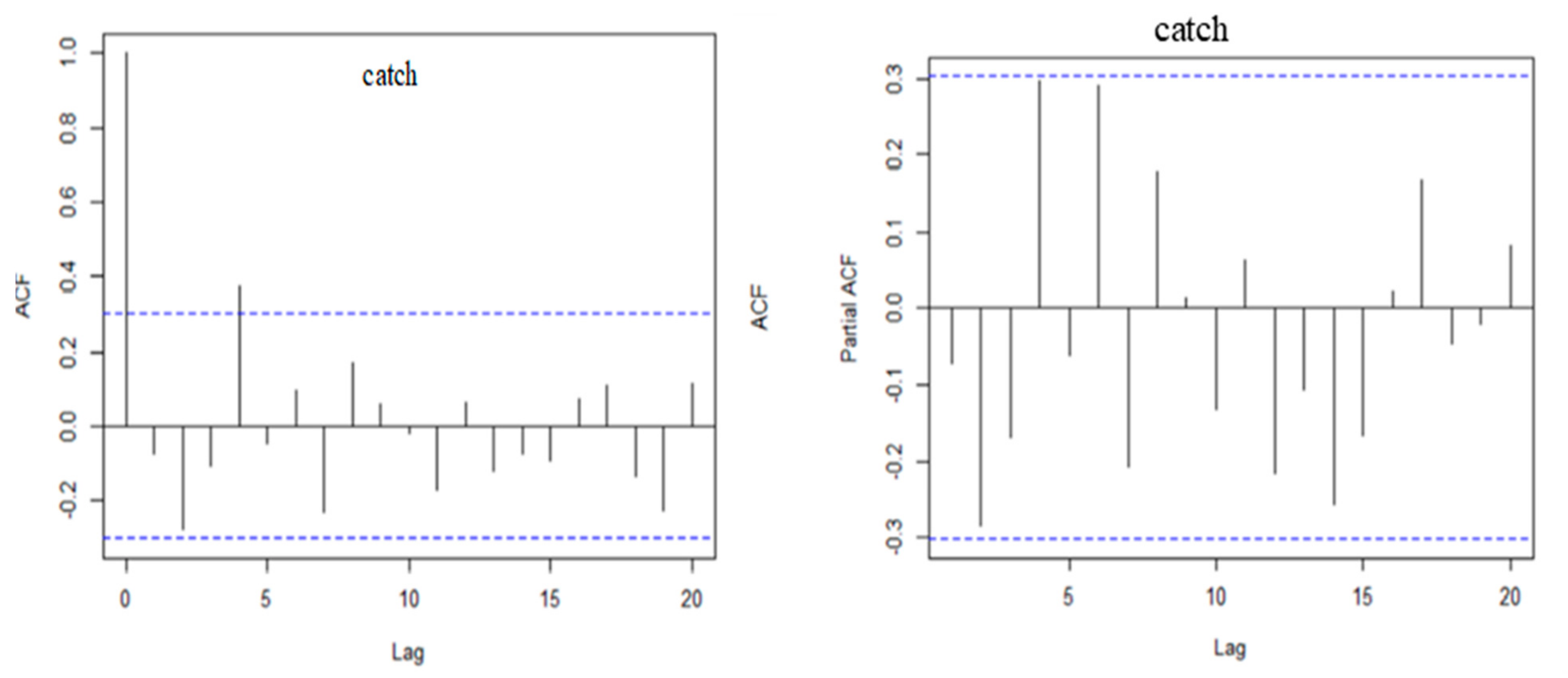
A correlogram was also applied to detect whether particular time series data was stationary or non-stationary. The stationary time series data give an AC and PAC functions that decay rapidly from their initial value of unity zero lag while in non-stationary time series, the ACF dies out gradually over time. The stationary testing was done using a plot analysis of the autocorrelation (ACF) and partial autocorrelation function (PACF). The ACF depicted the correlation measurement of the observations at different times. PACF coefficient also called reflection coefficients in signal processing was used as the basis of autoregressive estimation. The ACF and PACF of the transformed fish landings time series (original and smoothed series) are presented in Figure 5. Both fishery landings and CPUE data series showed that a first-order differencing (d = 1) was adequate to remove the trend. The ACF and PACF in Figure 5 showed a significant spike only at lag 1, meaning that higher-order autocorrelation was explained by lag 1 AR [26].
In verifying the data stationarity, however, it was noted that AR or MA models were not pure as seen from ACF and PACF correlograms in Figure 5. Therefore, several models had to be tested to identify the most suitable one for fishery landings and CPUE forecasting.

3.2. Model Selection

The model selection was based on the minimization of Akaike information criterion (AIC), Bayesian information criterion (BIC), square root of the mean square error (RMSE), the mean absolute error (MAE), standard error of prediction (SEP), average relative variance (ARV) and increasing Gaussian maximum likelihood estimation (GMLE) algorithm, efficiency coefficient E 2 and coefficient of determination ( R 2 ) . Table 1 summarizes the values of different competing models and proves the choice of the ARIMA (p,d,q) model on which fishery landings’ prediction was based on. Table 1 shows that the ARIMA model (0,1,1) had the lowest Akaike information criterion (AIC = 776.96), Bayesian information criterion (BIC = 780.49), square root of the mean square error (RMSE = 2001.29 tons), percentage standard error of prediction (SEP = 22%), average relative variance (ARV = 0.29), high Gaussian maximum likelihood estimation algorithm (GMLE = −386.48), and efficiency of coefficient E 2 (0.71).
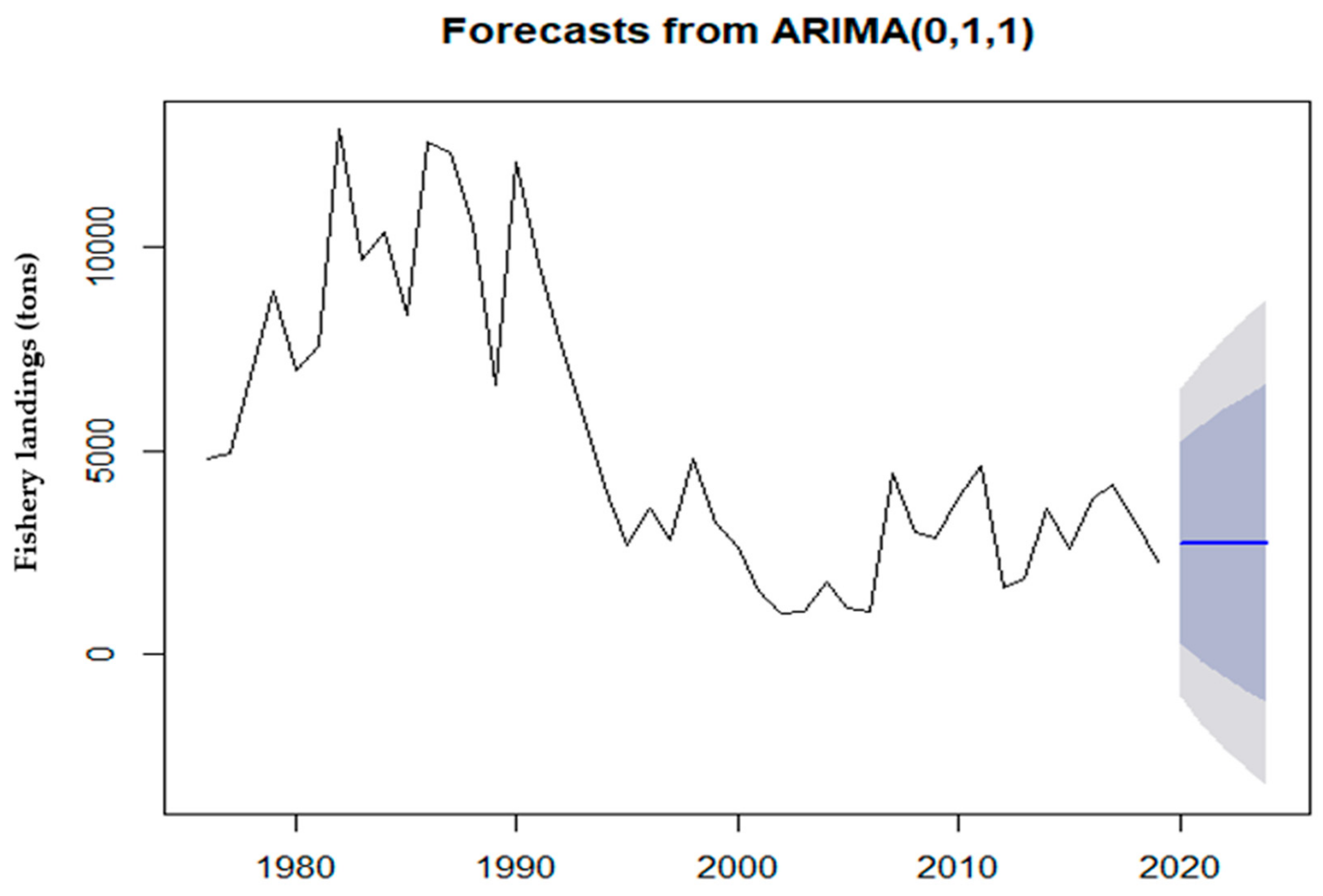
The coefficient of determination also known as R squared was used as an indicator for the goodness of model fit in the linear regression. The ARIMA (0,1,1) had the highest R2 coefficient (R2 = 0.73) suggesting that about 73% of the variance was explained by the model. Also, the persistent index (PI) was closer to 1 and higher (PI = 0.59) than the rest of the competing models suggesting that the ARIMA (0,1,1) model was not naïve. The p-value for the Ljung–Box test was greater than 0.05 suggesting that there was very little evidence for non-zero autocorrelations. Both AR and MA models were greater than 0.05, suggesting that the residues of the model were independent at a 95% level of confidence and the ARMA model proved to be the best model fit. The level of explained variance displayed a percentage standard error prediction (SEP) of 22%, root mean standard error (RMSE) of 2001.29 tons, and a mean absolute error of 1044.04 tons. A detailed analysis of the results showed that the model displayed the best performance as indicated by the persistence index which was closer to 1 (PI = 0.56). R statistical package version 3.6.3 has an installation for finding the appropriate forecasting model “auto. arima ()”. As seen from Figure 6, the ARIMA (0,1,1) was displayed as the most appropriate forecasting model for fish landings.
Table 2 on the other hand summarizes the measures of forecasting accuracy for CPUE among the competing ARIMA (p, d, q) models. According to the measures of forecasting used, the best forecasting performance was displayed by the ARIMA model (0,1,0). The model had lowest AIC (−44.24), BIC (−55.43), RMSE (0.08 kg/h), MAE (0.05 kg/h), SEP (26%), ARV (0.25), highest GMLE (39.6), E2 (0.6465), and PI (0.66). The R squared was used as an indicator for the goodness of model fit in the linear regression model. The ARIMA (0,1,0) had the highest R2 coefficient (R2 = 0.78) suggesting that about 78% of the variance was explained by the model. Also, the persistent index (PI) was closer to 1 and higher (PI = 0.66) than the rest of the competing models suggesting that the ARIMA (0,1,0) model was not naïve. The p-value for the Ljung–Box test was also greater than 0.05 suggesting that there was very little evidence for non-zero autocorrelations. Both AR and MA models were greater than 0.05 suggesting that the residues of the model were independent at a 95% level of confidence and the ARMA model proved to be the best model fit. Using the “auto. arima ()" command in R statistical package version 3.6.3, the software also automatically estimated ARIMA (0,1,0) as the best ARIMA model (Figure 6).
Based on the selected ARIMA (0,1,1) and ARIMA (0,1,0) models presented in Figure 6, the following model was developed.
y t = δ + δ 1 y t 1 θ 1 ε t 1 + ε t
with: y t , y t 1 : fish landings or CPUE period t and t − 1, respectively, ε t , ε t 1 : residuals of period t and t − 1 constitute a white noise, and δ 1 and θ 1 : coefficients of AR and MA processes, respectively.

3.3. Accuracy of ARIMA (0,1,1) and ARIMA (0,1,0) Models

Before forecasting, the residuals were checked through ACF and PACF to see if there was any systematic patterns that need to be eliminated to improve the accuracy and performance of the selected model. The ACF and PACF residuals plot (Figure 7) showed that none of the ACF were significantly different from zero at 95% confidence intervals. Therefore, ARIMA (0,1,1) and ARIMA (0,1,0) models provided an adequate predictive model which probably could not be improved.

4. Forecast

The modeled and predicted fish landings and CPUE are displayed in Figure 8. The summary of predicted and observed fish landings and CPUE are presented in Table 3 and Table 4. Table 3 and Table 4 show that the noise residuals were a combination of positive and negative errors and falling within 95% confidence intervals indicating that the model had a good performance of forecasting.
Figure 8 presents the results of fish landings and CPUE forecasts obtained after applying ARIMA (0,1,1) and ARIMA (0,1,0) models for the period of 5 years (2019–2024). As seen from Figure 8, the model satisfactorily predicted that by 2024, both fish landings and CPUE will be estimated at 2725.243 metric tons and 0.097 kg/h respectively.

5. Discussion

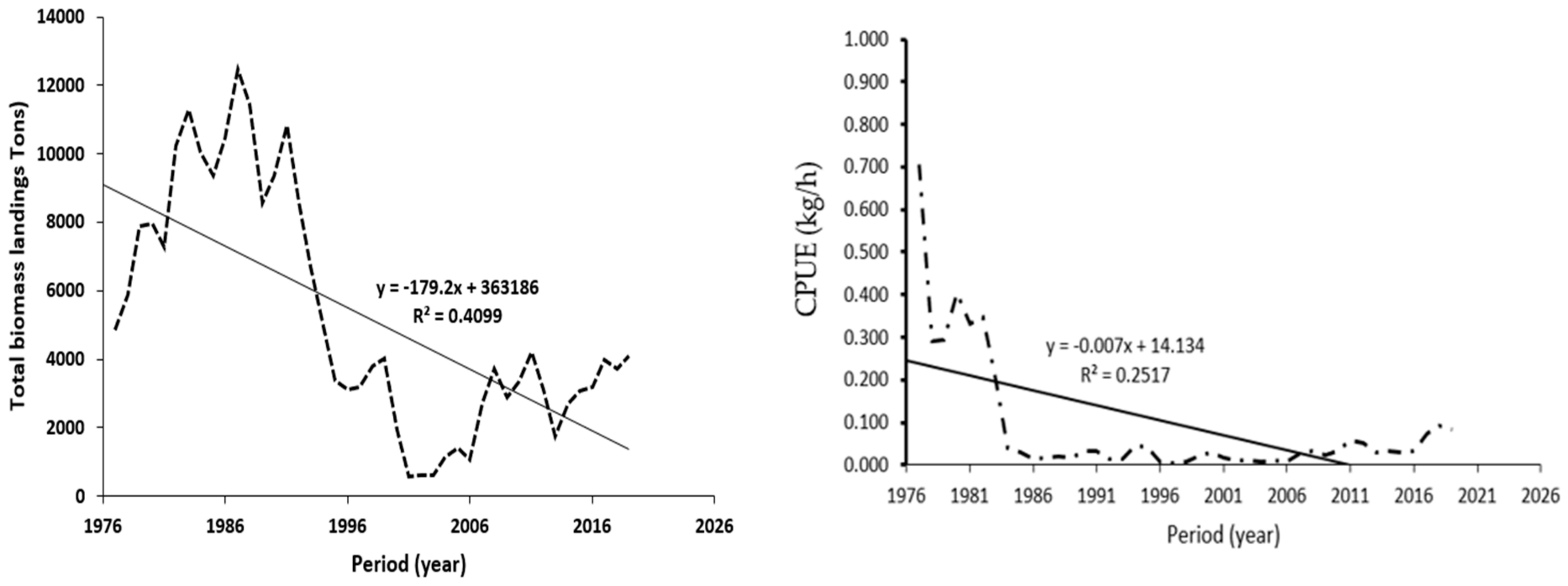
The abundance of fish species in Lake Malombe is directly linked to CPUE; though common criticism of CPUE is that the relationship between abundance and CPUE is more complex [28,29]. Figure 9 depicts the variation of the annual fish landings during each defined fish landing period. The data plot shows that Lake Malombe fish landings experience strong periodical fluctuations, with higher catches registered in 1976–1996 and maximum fish landings in 1984, and limited fish landings during the rest of the period. A significant decline in fishery landings is noted, during 2000–2005, mostly attributed to stock depletion as the result of an increase in fishing effort. The fishery recovery appeared from 2006 to 2016, with the maximum registered in 2015. The CPUE in Figure 9 was at the peak in 1976 and then began fluctuating negatively and thereafter remained constant with a slight fluctuation.
The decrease in CPUE trends from the 1980s to 2019 was an indicator of increasing fishing effort and a decrease in fish landings. Maynou et al. [30] explained that CPUE series reflect the general abundance of species and catch fluctuation. According to Weyl et al. [31], CPUE variation is strongly linked to the difference in the number of fishers, man-hours, and the categories of fishing gears. Low CPUE indicates a relatively low abundance of fish which results in prolonged man-hours and an increase in the number of fishers and low catches [32,33]. Alexander et al. [34] had similar observations and reported a strong relationship between whole lake CPUE to relative fish biomass and abundance. Weyl et al. [31] evidenced an increase in biomass and CPUE in the southern part of Lake Malawi after the subsequent closure of the fishery within 1992/1993. In Lake Nasser, Egypt, the time series of size and CPUE also showed a negative trend indicating the high exploitation rate of the most important commercial fish species in the lake by the fishing gears [32]. A similar situation is reported in Lake Chilwa, Lake Malawi, and other inland lakes [35,36,37].
The option to model both fishery landings and CPUE was based on the fact that these two indicators can be used by regulators to monitor for a potential change in fish population related to the effects of human exploitation and other anthropogenic factors [38]. It was based on the assumption that Lake Malombe fishery can provide a greater benefit to the riparian communities if proper management conditions and plans are sustainably exercised. Stergiou [38] claimed that fish landing fluctuation is linked to ecosystem type and season while Pinnegar et al. [39] believed that fish landings can reflect changes in gear technologies, management measures, and the species abundance in the lake ecosystem. The two arguments above indicate that the inaccurate model can give inaccurate management information and appropriate selection of the time series model is the basic requirement in the prediction of fish landings and CPUE. In this case, the ARIMA (0,1,1) and ARIMA (0,1,0) models were selected as the most accurate and the best in predicting Lake Malombe fish landings and CPUE for five years. It should be noted that the p = 0 in ARIMA (0,1,1) for fish landings suggests that there were no autoregressive terms but rather the model was exponential smoothing. On the other hand, the p = 0 and q = 0 in ARIMA (0,1,0) suggests that the selected model was a random walk with a constant trend and had no autoregressive and moving average terms. The five-year duration was chosen to increase the accuracy of the model. It was also assumed that forecasting five years in advance could be of great importance for planning and decision-making among fisheries managers, fishermen, and the fishing industry in general. The ARIMA (0,1,1) and ARIMA (0,1,0) models accurately predicted the lowest lake fish landings (2725.243 tons) and CPUE (0.097 kg/h), respectively. The prediction obtained by the models provides a special interpretation to fisheries managers, scientists, ecologists, and experienced fishers. It implies that the optimum fishing effort should be reduced below the current fishing effort for the fishery to recover a certain level of CPUE. In the absence of limitations, the open-access approach to the fishery in Lake Malombe will eventually lead to a further cycle of depression with declining economic returns for fishers and negative social and economic impacts [40].

6. Conclusions

In Malawi, fishing is described as the most productive and economic activity that sustains millions in the riparian communities. This study was developed to predict uncontrollable biomass trends and the possible abundance of the stock. The main objective was to provide baseline data to fisheries managers to set a practical fishing effort in the lake. The annual fish landings and CPUE trends were first transformed from non-stationary to stationary using the first-order differencing. The ACF, PACF, AIC, BIC, RMSE, MAE, SEP, ARV, GMLE, E2, R2, and PI were estimated, which led to the identification and construction of ARIMA models, suitable for explaining the time series and forecasting. According to the measures of forecasting accuracy, the best forecasting models for fish landings and CPUE were ARIMA (0,1,1) and ARIMA (0,1,0). These models had the lowest AIC, BIC, RMSE, MAE, SEP, and ARV values. The models further displayed the highest values of GMLE, PI, R2, and E2. The “auto. arima ()” command in R version 3.6.3 further displayed ARIMA (0,1,1) and ARIMA (0,1,0) as the best. The ARIMA (0,1,1) and ARIMA (0,1,0) models accurately predicted the lowest lake fish landings (2725.243 tons) and CPUE (0.097 kg/h), respectively, with a good level of confidence. The fish landings and CPUE trends showed downward trends suggesting that the current stock exploitation in Lake Malombe is unstainable. Therefore, the study recommends that the current fishing effort should be reduced to enable the fishery to recover a certain optimum level of CPUE.

7. Limitation

This study did not consider the use of hybrid models to explore the potential effects of covariates (such as fishing mortalities, environmental and social-economic drivers) due to limited data availability. Therefore, it is suggested that future studies should consider that.

Author Contributions

R.M. conceptualized the study, developed the methodology, sourced the data, analyzed the data, and developed the original manuscript. Authors S.M., E.K., T.A., T.B.P., I.B.M.K., C.C.K. supervised the study, reviewed and edited the manuscript, visualized, and validated the study. All authors have read and agreed to the published version of the manuscript.

Funding

This research was funded by the Federal Democratic Republic of Ethiopia through the African Centre of Excellence for Water Management, Addis Ababa University, Grant number GSR/9316/11.

Institutional Review Board Statement

Not applicable.

Informed Consent Statement

Not applicable.

Acknowledgments

The authors wish to thank the Department of Fisheries, particularly the Mangochi district fisheries office and Monkey Bay Fisheries Research, for providing fish biomass landings and CPUE data. Further acknowledgment is extended to the FAO-FiRM project, Mangochi Office, Malawi, for administrative support during the development of this manuscript.

Conflicts of Interest

The authors of this paper declare that there is no conflict of interest.

References

  1. Weyl, O.L.F.; Ribbink, A.J.; Tweddle, D. Lake Malawi: Fishes, fisheries, biodiversity, health and habitat. Aquat. Ecosyst. Health Manag. 2010, 13, 241–254. [Google Scholar] [CrossRef]
  2. Hara, M.; Njaya, F. Between a rock and a hard place: The need for and challenges to implementation of Rights Based Fisheries Management in small-scale fisheries of southern Lake Malawi. Fish. Res. 2016, 174, 10–18. [Google Scholar] [CrossRef] [Green Version]
  3. Government of Malawi. Fisheries Conservation and Management Act; Malawi Government: Lilongwe, Malawi, 1997.
  4. Hara, M.; Nielsen, J.R. Experiences with Fisheries Co-Management in Africa; Wilson, D.C., Nielsen, J.R., Degnbol, P., Eds.; Springer Nature: Dordrecht, The Netherdlands, 2003; pp. 81–97. [Google Scholar]
  5. Hara, M. Community response: Decline of the chambo in lake Malawi’s southeast arm. In Poverty Mosaics: Realities and Prospects in Small-Scale Fisheries; Jentoft, S., Eide, A., Eds.; Springer Science & Business Media B.V.: Berlin, Germany, 2011. [Google Scholar] [CrossRef]
  6. Njaya, F. Governance challenges for the implementation of co-management: Experiences from Malawi. Int. J. Commons 2007, 1, 137–153. [Google Scholar] [CrossRef]
  7. Lewy, P.; Nielsen, A. Modelling stochastic fish stock dynamics using Markov Chain Monte Carlo. ICES J. Mar. Sci. 2003, 60, 743–752. [Google Scholar] [CrossRef] [Green Version]
  8. Craine, M. Modelling Western Australian Fisheries with Techniques of Time Series Analysis: Examining Data from a Different Perspective; Department of Fisheries Research Division, Western Australian Marine Research Laboratories: North Beach, Australia, 2005. [Google Scholar]
  9. Stergiou, K. Prediction of the Mullidae fishery in the eastern Mediterranean 24 months in advance. Fish. Res. 1990, 9, 67–74. [Google Scholar] [CrossRef]
  10. Selvaraj, J.J.; Arunachalam, V.; Coronado-Franco, K.V.; Romero-Orjuela, L.V.; Ramírez-Yara, Y.N. Time-series modeling of fishery landings in the Colombian Pacific Ocean using an ARIMA model. Reg. Stud. Mar. Sci. 2020, 39, 101477. [Google Scholar] [CrossRef]
  11. Koutroumanidis, T.; Iliadis, L.; Sylaios, G.K. Time-series modeling of fishery landings using ARIMA models series modeling of fishery landings using ARIMA models. Environ. Model. Softw. 2006, 21, 1711–1721. [Google Scholar] [CrossRef]
  12. Park, H.-H. Analysis and prediction of walleye pollock (Theragra chalcogramma) landings in Korea by time series analysis. Fish. Res. 1998, 38, 1–7. [Google Scholar] [CrossRef]
  13. Georgakarakos, S.; Koutsoubas, D.; Valavanis, V.D. Time series analysis and forecasting techniques applied on loliginid and ommastrephid landings in Greek waters. Fish. Res. 2006, 78, 55–71. [Google Scholar] [CrossRef] [Green Version]
  14. Lloret, J.; Lleonart, J.; Solé, I. Time series modelling of landings in Northwest Mediterranean Sea. ICES J. Mar. Sci. 2000, 57, 171–184. [Google Scholar] [CrossRef] [Green Version]
  15. Prista, N.; Diawara, N.; Costa, M.J.; Jones, C.M. Use of SARIMA models to assess data-poor fisheries: A case study with sciaenid fishery of Portugal. Fish Bull. 2011, 109, 170–182. [Google Scholar]
  16. Raman, R.K.; Sathianandan, T.V.; Sharma, A.P.; Mohanty, B.P. Modelling and forecasting marine fish production in Odisha using seasonal ARIMA model. Natl. Acad. Sci. Lett. 2017, 40, 393–397. [Google Scholar] [CrossRef]
  17. Stergiou, K.I. Modelling and forecasting the fishery for pilchard (Sardina pilchardus) in Greek waters using ARIMA time-series models. ICES J. Mar. Sci. 1989, 46, 16–23. [Google Scholar] [CrossRef]
  18. Dulanya, Z.; Croudace, I.; Reed, J.M.; Trauth, M.H. Palaeoliminological reconstruction of recent environmental change in Lake Malombe (S.Malawi) using multiple proxies. Water SA 2014, 40, 1–12. [Google Scholar] [CrossRef] [Green Version]
  19. Matiya, G.; Wakabayashi, Y. Small scale fisheries of Malawi: An outline of Lake Malombe fisheries. Mem. Fac. Agric. Ehime Univ. 2005, 50, 3–9. [Google Scholar]
  20. Petrere, M., Jr.; Giacomini, H.C.; De Marco, P., Jr. Catch-per-unit-effort: Which estimator is best? Braz. J. Biol. 2010, 70, 483–491. [Google Scholar] [CrossRef] [PubMed] [Green Version]
  21. Thompson, S.K. Sampling; Wiley: New York, NY, USA, 1992. [Google Scholar]
  22. Griffiths, R.C. A study of measures of population density and the concentration of fishing effort in the fishery for yellowfin tuna, Neothunnus macropterous, in the Eastern tropical Pacific Ocean, from 1951 to 1956. Inter-Am. Trop. Tuna Comm. Bull. 1960, 4, 41–96. [Google Scholar]
  23. Snedecor, G.W.; Cochran, W.G. Statistical Methods, 6 ed.; The Iowa State University Press: Ames, IA, USA, 1967. [Google Scholar]
  24. Gutiérrez-Estrada, J.C.; Silva, C.; Yáñez, E.; Rodríguez, N.; Pulido-Calvo, I. Monthly catch forecasting of anchovy Engraulis ringens in the north area of Chile: Non-linear univariate approach. Fish. Res. 2007, 86, 188–200. [Google Scholar] [CrossRef]
  25. Makwinja, R.; Singini, W.; Kaunda, E.; Kapute, F.; M’balaka, M. Stochastic modeling of Lake Malawi Engraulicypris sardella (Gunther, 1868) catch fluctuation. Int. J. Fish. Aquac. 2018, 10, 34–43. [Google Scholar]
  26. Box, G.E.P.; Jenkins, G.M. Time Series Analysis: Forecasting and Control.; Holden Day: Oakland, CA, USA, 1976. [Google Scholar]
  27. Mgaya, J.F.; Yildiz, F. Application of ARIMA models in forecasting livestock products consumption in Tanzania. Cogent Food Agric. 2019, 5, 1607430. [Google Scholar] [CrossRef]
  28. Harley, S.J.; Ransom, A.M.; Dunn, A. Is catch-per-unit-effort proportional to abundance? Can. J. Fish. Aquat. Sci. 2001, 58, 1760–1772. [Google Scholar] [CrossRef]
  29. Guzzo, M.M.; Rennie, M.D.; Blanchfield, P.J. Evaluating the relationship between mean catch per unit effort and abundance for littoral cyprinids in small boreal shield lakes. Fish. Res. 2014, 150, 100–108. [Google Scholar] [CrossRef]
  30. Maynou, F.; Demetre, M.; Sánchez, P. Analysis of catch per unit effort by multivariate analysis and generalized linear models for deep-water crustacean fisheries off Barcelona (NW Mediterranean). Fish. Res. 2003, 65, 257–269. [Google Scholar] [CrossRef]
  31. Weyl, O.; Mwakiyongo, K.; Mandere, D. An assessment of the nkacha net fishery of Lake Malombe Malawi. Afr. J. Aquat. Sci. 2004, 29, 47–55. [Google Scholar] [CrossRef]
  32. El-Far, A.; Aly, W.; El-Haweet, A.E.-D.; Nasr-Allah, A.; Karisa, H. Fisheries management based on gear selectivity of a tropical reservoir, Lake Nasser, Egypt. Egypt. J. Aquat. Res. 2020, 46, 71–77. [Google Scholar] [CrossRef]
  33. Solomon, S.G.; Ayuba, V.O.; Tahir, M.A.; Okomoda, V.T. Catch per unit effort and some water quality parameters of Lake Kalgwai Jigawa state, Nigeria. Food Sci. Nutr. 2018, 6, 450–456. [Google Scholar] [CrossRef] [Green Version]
  34. Alexander, T.J.; Vonlanthen, P.; Periat, G.; Degiorgi, F.; Raymond, J.; Seehausen, O. Estimating whole-lake fish catch per unit effort. Fish. Res. 2015, 172, 287–302. [Google Scholar] [CrossRef]
  35. Kidd, K.A.; Blanchfield, P.J.; Mills, K.H.; Palace, V.P.; Evans, R.E.; Lazorchak, J.M.; Flick, R.W. Collapse of a fish population after exposure to a synthetic estrogen. Proc. Natl. Sci. USA 2007, 104, 8897–8901. [Google Scholar] [CrossRef] [PubMed] [Green Version]
  36. Njaya, F.; Snyder, K.A.; Jamu, D.; Wilson, J.; Howard-Williams, C.; Allison, E.H.; Andrew, N.L. The natural history and fisheries ecology of Lake Chilwa, southern Malawi. J. Great Lakes Res. 2011, 37, 15–25. [Google Scholar] [CrossRef]
  37. Makwinja, R.; Chapotera, M.; Likongwe, P.; Banda, J.; Chijere, A. Location and roles of deep pools in Likangala river during 2012 recession period of Lake Chilwa basin. Int. J. Ecol. 2014, 2014, 1–4. [Google Scholar] [CrossRef] [Green Version]
  38. Stergiou, K.I. Overfishing, the tropicalization of fish stocks, uncertainty, and ecosystem management: Resharpening Ockham’s razor. Fish. Res. 2002, 55, 1–9. [Google Scholar]
  39. Pinnegar, J.K.; Polunin, N.V.C.; Badalamenti, F. Long-term changes in the trophic level of western Mediterranean fishery and aquaculture landings. Can. J. Fish. Aquat. Sci. 2003, 60, 222–235. [Google Scholar] [CrossRef]
  40. FAO. Fisheries Management; FAO Technical Guidelines for Responsible Fisheries. No. 4; Food and Agriculture Organization of the United Nations: Rome, Italy, 1997. [Google Scholar]
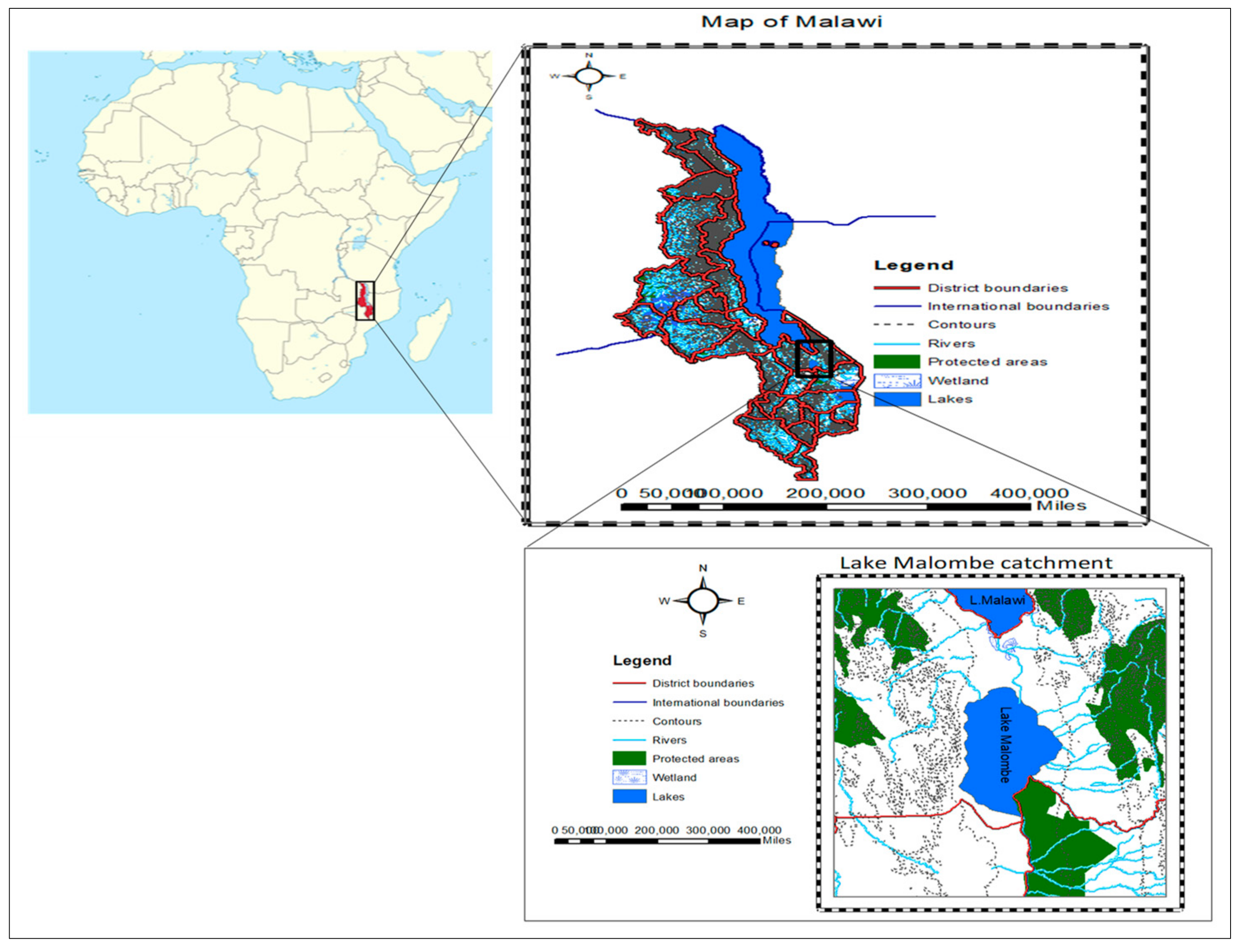
Figure 1. Map of Lake Malombe.
Forecasting 03 00004 g001
Figure 2. Total biomass landings (tons) and catch per unit effort (kg/h).
Forecasting 03 00004 g002
Figure 3. Autocorrelation and partial autocorrelation functions of original fishery landings and CPUE.
Forecasting 03 00004 g003
Figure 4. First order differences.
Forecasting 03 00004 g004
Figure 5. Autocorrelation (AC) and partial autocorrelation (PAC) functions.
Forecasting 03 00004 g005
Figure 6. Estimated values for ARIMA (0,1,1) (a) and ARIMA (0,1,0) (b).
Forecasting 03 00004 g006
Figure 7. Autocorrelation and partial autocorrelation functions residuals.
Forecasting 03 00004 g007aForecasting 03 00004 g007b
Figure 8. Forecast fish landings and CPUE from 2019 to 2024.
Forecasting 03 00004 g008aForecasting 03 00004 g008b
Figure 9. Biomass and CPUE trend.
Forecasting 03 00004 g009
Table 1. Competing autoregressive integrated moving average (ARIMA) models for total annual fish landings.
Model (p,d,q)R2RMSE (tons)MAE (tons)BICAICLog-LikelihoodSEP (%)ARVE2PILjung–Box (p-Value)
ARIMA (0,1,0)0.692035.371507.99815.50777.96−386.49320.330.670.230.49
ARIMA (1,1,1)0.692035.241514.83795.50778.95−389.48440.330.67 0.130.63
ARIMA (2,1,2)0.692067.421518.65795.61779.60−386.76560.340.660.140.89
ARIMA (2,2,2)0.702107.421494.62815.83777.65−398.82530.350.650.440.48
ARIMA (0,1,1)0.732001.291044.04780.49776.96−386.48220.290.710.560.64
ARIMA (2,0,0)0.662015.741474.24915.06788.68−389.34760.320.680.390.65
R2 means coefficient of determination, RMSE means square root of the mean square error, MAE means mean absolute error, BIC means Bayesian information criterion, AIC means Akaike information criterion, SEP means percentage standard error of prediction, ARV means average relative variance, E2 means efficiency Coefficient, PI means persistent index.
Table 2. Competing ARIMA models for CPUE.
Model (p,d,q)R2RMSE (kg/h)MAE (kg/h)BICAICLog-LikelihoodSEP (%)ARV E2PILjung–Box (p-Value)
ARIMA (0,1,0)0.750.080.05−55.43−57.1939.6260.250.64650.660.589
ARIMA (1,1,1)0.740.110.06−44.08−53.6829.84440.370.62640.380.844
ARIMA (2,1,2)0.720.100.06−47.09−55.6734.84470.39 0.60570.290.707
ARIMA (2,2,2)0.570.120.07−45.08−54.8832.44640.36 0.63980.470.717
ARIMA (0,1,1)0.750.110.06−49.14−43.9424.97540.43 0.57010.320.787
ARIMA (2,0,0)0.750.130.07−36.68−42.54−35.34920.430.57000.340.645
R2 means coefficient of determination, RMSE means square root of the mean square error, MAE means mean absolute error, BIC means Bayesian information criterion, AIC means Akaike information criterion, SEP means percentage standard error of prediction, ARV means average relative variance, E2 means efficiency Coefficient, PI means persistent index.
Table 3. Forecast total fish annual biomass landings from 2019 to 2024.
YearForecastLo 80Hi 80Lo 95Hi 95
20202725.243147.2225203.265−1064.5636515.05
20212725.243−185.1475635.634−1725.8147176.301
20222725.243−561.1156011.602−2300.8097751.295
20232725.243−898.2826348.769−2816.4608266.947
20242725.243−1206.646657.128−3288.0558738.542
Table 4. Forecast CPUE from 2019 to 2024.
YearForecastLo 80Hi 80Lo 95Hi 95
20200.097−0.0590.252−0.1410.335
20210.097−0.1230.317−0.2400.434
20220.097−0.1730.367−0.3160.509
20230.097−0.2150.409−0.3800.574
20240.097−0.2510.445−0.4360.629
Publisher’s Note: MDPI stays neutral with regard to jurisdictional claims in published maps and institutional affiliations.