3.1. Representation
Earthquake occurrences have been modeled using a variety of point process models and the most popular is the Epidemic Type Aftershock Sequence (ETAS) model. In this model, events are divided into two categories. There are background events and triggered events. Background events are events that occur spontaneously. Triggered events occur as a result of other events. Each event can trigger new events, which in turn can again trigger new events. [
11] provide a list of common features of ETAS models, and these are: (a) the occurrence rate of background events depends on location and magnitude, but is independent of time; (b) the magnitude of a background event is independent of its location; (c) each event produces offspring events independently and the number of offspring events produced depends on the magnitude of the event; (d) the occurrence time of an offspring event depends only on the time difference from its ancestor and is independent of the magnitude; (e) the location of an offspring event depends on the location of its ancestor; and (f) the magnitude of an offspring event is independent of the magnitude of its ancestor. These six features explain the design of the ETAS model.
One of the first models is the temporal ETAS model proposed by [
9] to describe the origin times and magnitudes of earthquakes. This model has been extended to also include the spatial aspect of earthquake occurrences in [
10] and [
11]. Below, we will use this spatial-temporal ETAS model for the social conflicts.
The occurrences of events can often be completely described by the conditional intensity function of the process, which gives the probability of an event with a certain magnitude occurring at a specific place at a specific time. This function often consists of two parts, that is, a part describing the occurrence rate of background events and another part describing the way events trigger new events.
In our study we use the model as defined in [
8], which is similar to the one in [
10]. The conditional intensity function in this model is given by:
where event
i is described by a time
, location
and magnitude
. This intensity function consists of three parts, that is, the spatial background distribution
, the decay function
) and the magnitude probability density function
. Each of these components will be discussed next.
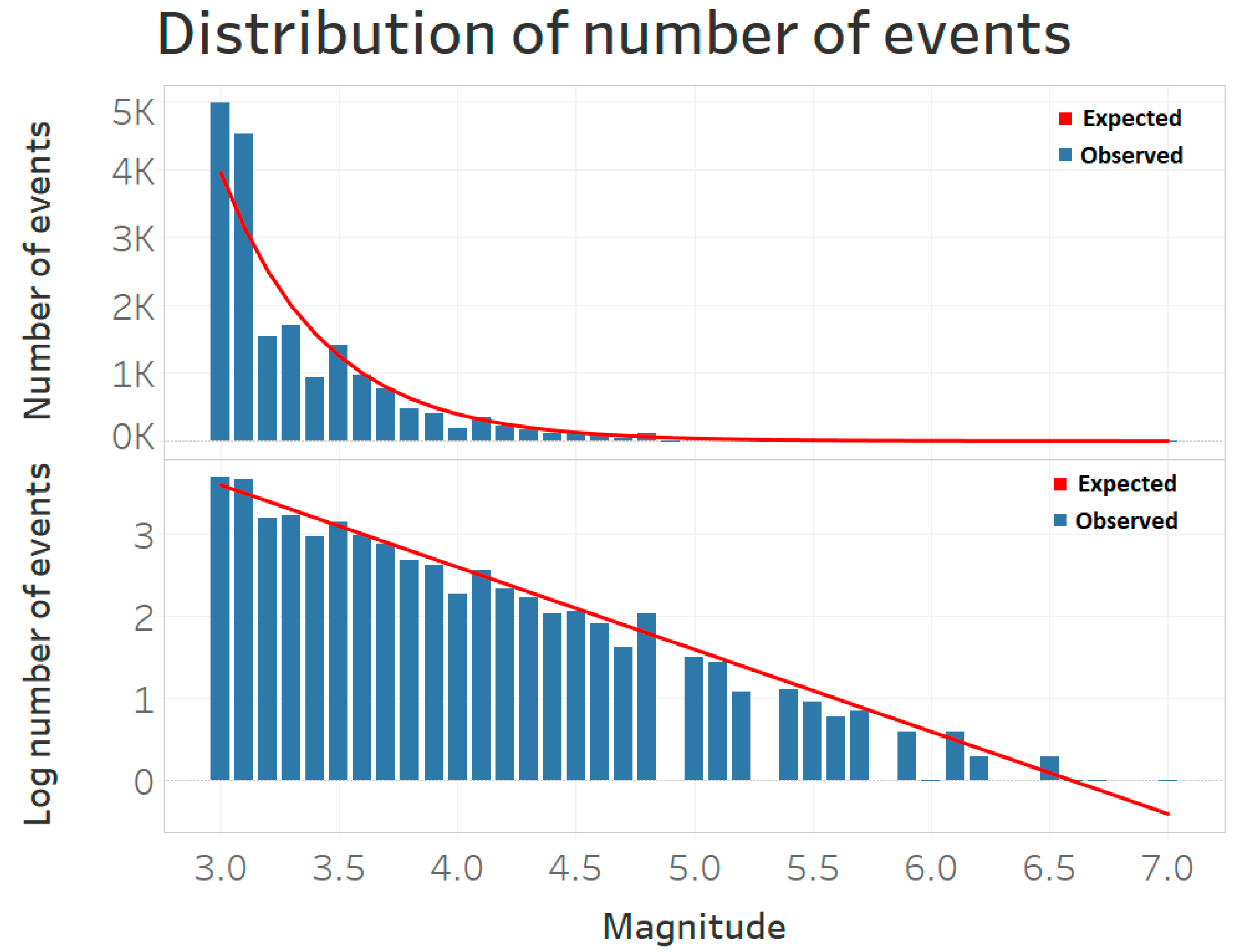
The magnitude probability density function is based on the Gutenberg–Richter law (hence the reason to scale that data as in the
Appendix A) and is given by:
where
and
is the magnitude of the largest event. The
refers to the minimum magnitude for which the catalog is complete, that is, the magnitude for which all events with magnitude
are recorded.
The rate at which event
i can trigger new events decreases with distance and time from that event. This is described by the decay function
) which is given by:
Here,
is the history of events before event
i. The decay function in (4) consists of two parts. The first part describes the temporal decay rate and the second part the spatial distribution. The temporal decay is governed by the parameters {
}. The parameter
measures the influence of excess magnitude
in generating offspring events and
k is a normalizing constant for the number of offspring events. A small value for
implies that the effect of the magnitude on triggering new events is small, and thus that smaller events can trigger a larger amount of events more easily, see [
12]. As usual, we assume that larger events cause more aftershocks than smaller events, that is,
. As the number of offspring events cannot be negative, we have that also
k > 0. It is hard to register all aftershocks after a large event and this incompleteness is measured by the parameter
c. Finally, the parameter
p is the rate of decay over time. We would expect
p > 1, as this implies that each event can only generate a finite number of offspring events.
The second part of (4) determines the spatial probability distribution. The term
is the distance to event
i and
is a normalization constant such that the integral over the entire region equals 1. The term
measures the influence of magnitude on the spatial extent of the aftershock region for event
i. Similar to
p, the parameter
q measures the spatial decay rate. If we ignore any spatial components in the model and integrate over the entire region, the right-hand term of (4) becomes 1 and we obtain the decay function for the temporal model in [
9].
The first term in (2) consists of a parameter
and the spatial background distribution
u(x, y). The parameter
is the Poisson rate of background events. The background distribution determines how these events are distributed across the region. We will estimate the spatial background distribution following the procedure in [
8], which is largely based on the iterative kernel method proposed by [
13]. For this, the region of interest is first divided into
cells
to make a discrete approximation. The cells are of size 0.5 × 0.5 degrees latitude/longitude, which corresponds to an area of approximately 55 × 55 = 3025 square kilometers. The background rate can vary among cells but is assumed to be homogeneous within each cell. We can then write
where
is the probability of a background event occurring in cell
i with area
.
The probabilities
are estimated using the iterative kernel method proposed by [
13], which uses the following function for the background distribution, that is,
where
T is the length of the study period,
N the total number of events,
is the probability that event
j is a triggered event and
is a variable bandwidth. The probability
is given by the ratio between the intensity produced by all previous events and the total intensity at that time and place, that is,
Finally,
is a variable bandwidth defined as the smallest disk around event
j which includes at least
events, as in [
11]. This way, events happening in rural areas have a further reaching effect than events that happen in densely populated areas, which makes regions with high and low event densities more comparable. Following [
14], we can use (5) to estimate the probabilities
by:
These probabilities then give the spatial background distribution, where the sum over all cells equals 1. Together with the average background rate , the decay function and the magnitude distribution f (m), we now have described the conditional intensity function of the process. This function will be used for calculating the maximum log likelihood which gives the parameter estimates.
The log-likelihood function is given by [
11], and it reads as:
For the calculation of the log likelihood, the background probabilities from (7) are needed for the cells in which an event has taken place.
Hence, the parameters of the model are where is the subset of nonempty cells. These parameters can be estimated by maximizing the log likelihood function using the simulated annealing algorithm, which will be discussed below.
Due to the high dimensionality of the likelihood function, there is a chance that a parameter is not identified and becomes arbitrarily large or small during the estimation. Therefore, we will impose certain parameter restrictions on the eight parameters in the model. These restrictions are based on the restrictions used for modeling earthquake occurrences and on values that are physically desirable, see [
10]. These restrictions are given in
Table 3. The branching ratio of the process gives the average number of events triggered by an event and is given by [
8] and equals:
If due to , events are generated faster than they die out and the process becomes explosive. The four parameters in the temporal component, , p, c, and k influence the number of events in the simulated catalogs. Furthermore, the parameter has a positive linear effect on the number of events and the parameters that determine the spatial decay, d, and q have no effect on the number of events. The spatial parameters describe the distribution of the events over the region. A higher value for and k lead to more events and a higher value for c leads to fewer events. For the temporal decay rate p there is a small region in which the process is not explosive. However, the size of this parameter region varies depending on the values of the other parameters.
3.2. Estimation
The parameters will be estimated using a simulated annealing algorithm, which is a method for approximating the global optimum of a given function. It originates from annealing in metallurgy, describing the physical process of reducing defects by heating and then slowly cooling the material. Even though this method is unlikely to find the optimal solution, it can often find a very good approximation of the optimum. In particular, it can be preferable over (quasi) Newton methods in situations with a large number of independent variables like in our case. As the algorithm finds a good solution in a relatively short amount of time, we can run it many times, providing a probability distribution for the parameters and the background distribution. These can be used to evaluate model uncertainties. We will run the algorithm times.
The algorithm starts by generating a random solution, after which it searches for a new point in that neighborhood. This search is based on a probability distribution that depends on the so called temperature of the process. The method accepts all points that raise the objective function (in case of maximization) and also accepts points that lower the objective, with a certain probability. As such, it avoids being trapped in local maxima. By decreasing the temperature, the probability of accepting a worse solution is lowered when the solution space is explored.
More formally, we adopt the simulated annealing procedure used to estimate the ETAS models as described in [
13]. It consists of an initialization, a loop and a cooling scheme.
To initialize set the count
and generate a random starting point
and set the initial temperature
. The starting temperature must be high enough that any solution can be selected and is calculated based on the function to be optimized, see [
15].
The loop is a random search for a better solution around the local maximum. First, set
and generate the next candidate
from a multi-dimensional Cauchy distribution G. We move to this point with a certain probability. Sample
uniformly and move to the newly generated point if
, where the acceptance function
A is the Metropolis criterion in [
16], that reads as:
If the log-likelihood at this new point is larger, we set this new point as the current optimum, that is,
Once a new optimum is found, the temperature is lowered according to the cooling schedule proposed in [
8], that is,
where
D = 8 is the number of parameters in the model. The two constants −13.8 and 3.4 were found to provide a fast algorithm based on a simulation study in [
8]. After decreasing the temperature, the loop is repeated until convergence. Events that took place before the study period can still have an effect on events inside the study period. We will therefore use a one year burn-in period when estimating the model. Hence, the estimation period consists of five years from 2012 to 2016, where 2012 will be used as a learning period and the four other years, 2013–2016, will be used as the study period. The data of the last year 2017 will be used for evaluating out-of-sample forecast performance.
3.3. Inference
If the model describes the dynamics of the conflicts well, the residuals are expected to follow a stationary Poisson process with a unit rate. The residuals are obtained by a transformation of the time axis, as in [
16], that is,
These residuals give the expected number of events with magnitude larger than up to time t and in the region R. If the residuals follow a stationary Poisson process with rate one, the inter-event times follow an exponential distribution. This can be tested using a one-sided Kolmogorov–Smirnov test (KS-test). We will also perform a Wald–Wolfowitz runs test, which tests the null hypothesis that the inter-event times are stationary and not autocorrelated.
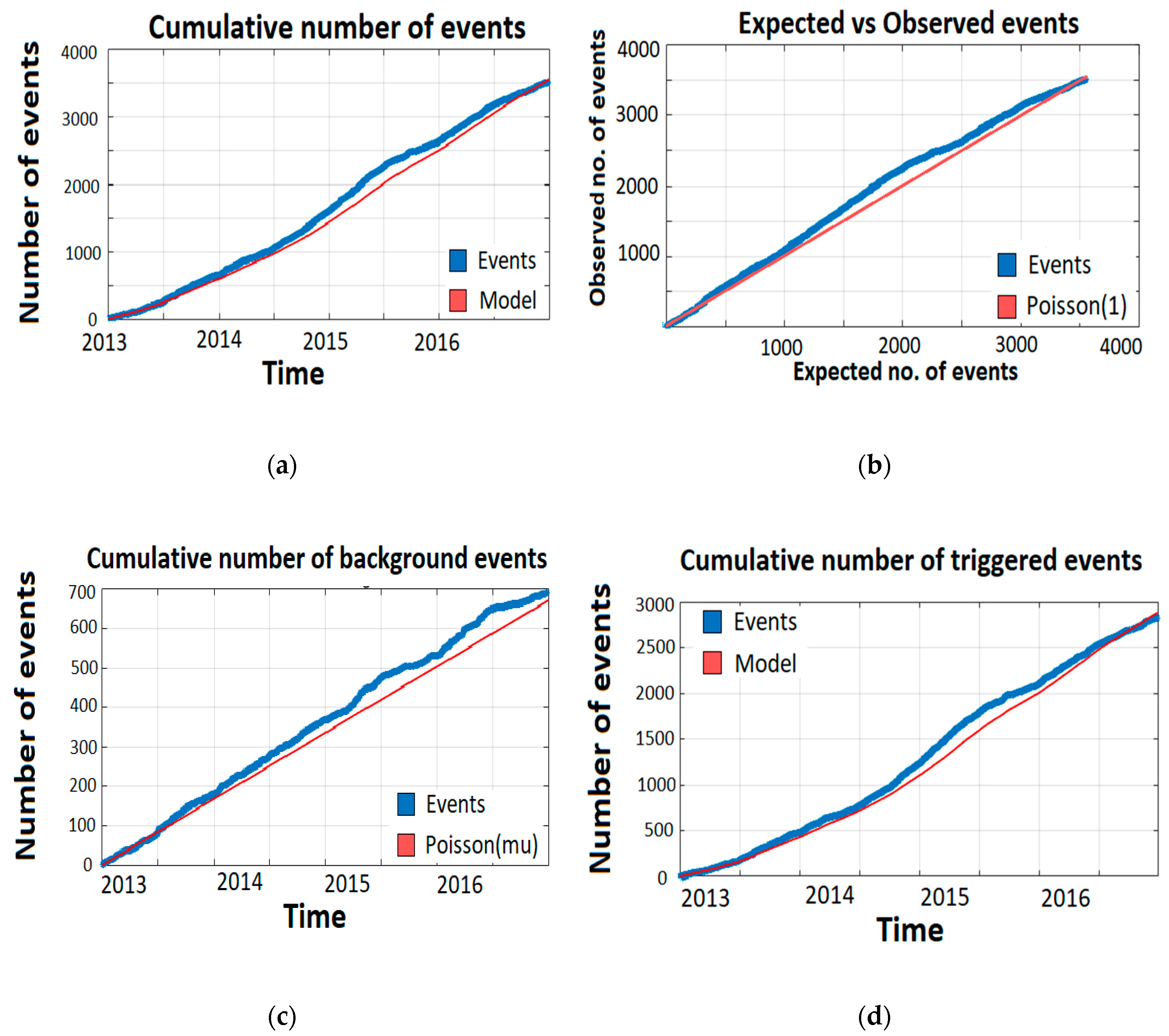
Furthermore, we can perform a visual check by plotting the number of events expected by the model against the observed number of events. This can be done for the transformed times, all events, background events and triggered events. The expected numbers of events are calculated by integrating the intensities over time, magnitude and space. The expected number of total events is given by:
The expected number of background events is given by:
and the expected number of triggered events is:
where
and
are the start and end times of the sample period. Note that we also integrate over the magnitude distribution, but as the magnitudes are independent of the parameters, this integral equals one.
The observed number of all events (background + triggered) can be obtained directly. As we cannot know for certain whether an event is a background or a triggered event, we cannot count them. Therefore, the number of observed background and triggered events are calculated as the sum of the probabilities of being a background or triggered event. The probability that event
i is a background event is given in [
8], and it reads as:
and the probability that event
i is a triggered event is given by
. The sum of these probabilities over all events determine the ‘observed’ number of background and triggered events.
The number-of-events test compares the number of events in the conflict catalog (the dataset) with the number of events expected by the model. The expected number of events and its distribution are obtained from simulating a large number of event catalogs and calculating the number of events in each of them. Specifically, this is done in the following way. Simulate catalogs based on the estimated parameters in an ETAS model. Then, fit a normal distribution to the number of events in each simulated catalog. Next, calculate the median and the 95% confidence bounds, and with these we compute the probability that we observe more events than in our dataset.
Finally, we will test the performance of the model by making a forecast for the number of events and their location in the hold-out sample. We focus on events with magnitude
, which for the African countries data corresponds to 22 or more fatalities. For this, we simulate
catalogs using the empirical ETAS model and calculate the expected number of events with magnitude
in each cell of the regions in the hold-out sample. The expected number of events in simulated catalog
i in cell
is given in [
8], and it reads as:
where
is the history of the process up to time
t for catalog
i. For each cell we then take the median number of events of all simulated catalogs as the forecast. The total number of events can then be calculated as the sum of the median number of events over all cells. The forecasted number of events and locations will then be compared with their observed number and locations to examine accuracy.
In [
13], the above described estimation and evaluation methodology is examined using extensive simulations. There it is concluded that the ETAS model can be reliably implemented for simulated data. It can happen though that parameters are estimated at their boundary value, and this is not unexpected given that the ETAS model is heavily parameterized.


