1. Introduction
Electricity price forecasting is a branch of energy forecasting that focuses on predicting the spot and day-ahead prices in the electricity market. Price forecasting is one of the fundamental tasks in utilities and energy trading entities for various decision-making mechanisms, for example, adjusting bids to maximize profits, scheduling outages and establishing load profiles. In particular, more accurate short-term price forecasts benefit both producers and consumers, as they can maximize profit and minimize the cost of a variety of applications such as home energy management programs in dynamic pricing environments and demand response. Electricity price is highly unstable in the open market or for consumers and its instability further increases by the deployment of the smart grid as it is influenced by many visible and invisible factors. For example, short-term price (e.g., hourly scales) depends on current demand, type of energy used for generation, historical price trend, hour of days and so forth. Medium term (weekly scales) and Long-term price (monthly to yearly scales) is influenced by factors like energy reserve (oil and gas), expected demand, population growth and various economic factors. Most of the research on price prediction uses these factors as input features for prediction models.
This spot electricity market is a day-ahead market, unlike the commodity market which allows for continuous trading. In this market, an agent submits its price bid for the next day before the market bid closing time and usually is cleared by the market operator after a market clearing optimization process is performed. A 1% saving in the MAPE (Mean Absolute Percentage Error) accuracy of a Short-term price forecast (STPF) is approximately equal to
$300,000 in savings per year per GW peak-load. However, due to lots of factors, such as energy policy, urban population, socio-economical activities, weather conditions, holidays and so on [
1], the electric load data display seasonality, non-linearity and a chaotic nature, which complicates electric load forecasting work [
2]. Thus, a reduction in MAPE is of importance to traders and transmission planners, such as for evaluating the magnitude and patterns of congestion in the system. Price forecasting approaches are often based on multi-agent, fundamental, reduced form, statistical, or machine learning techniques [
3].
The conventional statistical models, which include the Auto-Regressive Integrated Moving Average (ARIMA) models [
4,
5], regression models [
6,
7], exponential smoothing models [
8], Kalman filtering models [
9], Bayesian estimation models [
10,
11] and so on use historical data to find out the linear relationships among time periods. The methods such as artificial neural networks (ANNs) [
12,
13], expert system models [
14,
15] and fuzzy inference systems [
16,
17] have been widely applied to improve the performance of electric load forecasting. In [
18], authors use Support Vector Regression (SVR) with chaotic cuckoo search (SSVRCCS) model, improves the forecasting accuracy level by capturing the non-linear and cyclic tendency of electric load changes. In [
19], authors propose a method for short-term price forecasting using self-organized map (SOM). They use a two-stage method, SOM network is used in the first stage and support vector machine is used to fit the output from SOM to each subset in the second stage in a supervised manner. Having removed the anomalies from the training set they obtained mean absolute percentage error (MAPE) as 10.24% in hybrid network approach for the ISO New England market in [
20], Martinez-lvarez et al. presented a method which was based on pattern sequence similarity. In this approach, a clustering technique was first used on the data before application of the Pattern Sequence-based Forecasting (PSF) algorithm to produce one step ahead forecasts of the electricity prices. In [
21], the authors proposed fuzzy inference net (FIN) method for price forecasting, the proposed method uses FIN to extract fuzzy rules with Fuzzy Self-organization Mapping (FSOM) to evaluate the probability of unknown data for the predetermined cluster.
In this paper, we propose a two stage model with Auto-Regressive Integrated Moving Average (ARIMA) as the standard method for Stage-1, as it captures temporal, trend and seasonality information more accurately than other existing methods. ARIMA is a well-known method for predicting time-series data sets. In Stage-2 of the proposed model, machine learning techniques such as Random Forest (RF), Support Vector Machine (SVM), Locally Weighted Scatterplot Smoothing (LOWESS) and Generalized Linear Model (GLM) for better MAPE values are used.
ARIMA has been extensively used for load forecasting applications and as the key method for forecasting short-term electricity price predictions. L. Wu et al. [
22] presented a hybrid model for day-ahead electricity market clearing price by using a combination of time-series and adaptive wavelet neural network (AWNN). This model utilized an autoregressive moving average with exogenous variables (ARMAX) model to find the relationship between price return series and explanatory variable load series and a generalized autoregressive conditional heteroscedastic (GARCH) model to generate the residual characteristics. The authors also utilized Monte Carlo simulation method to generate a random number for time-series and AWNN models to improve the convergence rate. L. Wu et al. [
23] developed a two-stage integrated load and price forecast model for the New York Independent System Operator (NYISO) market. The initial stage forecast considered the load and price forecast separately. The second stage evaluated the price and load forecast interaction using the initial forecast as input, with each stage utilizing a hybrid time series and AWNN combination. ARIMA model was utilized to capture the linear relationship between price and load series and the residuals were evaluated using the GARCH model. The main contribution from the paper is that the authors have used an iterative prediction procedure to analyze the interaction between the load and price signals. This framework was used to forecast to the day-ahead price based on the historical data.
In [
24], authors combined a time-varying regression model with ARMA in a two-stage model after accounting for the impact of system load and wind power generation in the Western Danish price area of Nord Pool’s Elspot. In the first stage, the non-linear and non-stationery influence of the explanatory variables is accommodated using a time-varying regression model. In the second stage of the model, authors have used a time series model such as ARMA and Holt-winters to account for residual autocorrelation and seasonal dynamics. In [
25], the authors have used a wide variety of methods to compare the predictive accuracy for the day-ahead spot price of the Spanish electricity market. The authors used the double seasonal ARIMA as a univariate method along with exponential smoothing and both are used as a benchmark for comparison with the multivariate methods such as feed-forward neural networks which include the explanatory variables such as wind generation and weekdays. The results show that the exponential smoothing performed better than ARIMA, although they performed differently as the horizon increases. The authors have shown that the inclusion of the wind generation forecast as the explanatory variable has significantly increased the predictive accuracy of the dynamic regression model. The authors were able to obtain improvement in accuracy through the novel periodic model in relative to the dynamic regression model. In [
26], authors proposed an improved hybrid forecasting model for New South Wales in Australia that detaches high volatility and daily seasonality based on empirical mode decomposition, seasonal adjustment and ARIMA. The authors have compared the proposed hybrid model with the traditional ARIMA model and found that the prediction errors were reduced noticeably. These models were tested for forecasting the Half-hourly electricity prices. In [
27], authors compared the accuracies of twelve time-series methods for California and Nordic markets. These methods include standard auto regression and their extension spike preprocessed, threshold and semiparametric auto regressions as well as mean-reverting jump diffusion. These methods were tested with time-series data of system-wide load and hourly spot prices for the California market, while hourly spot prices and air temperature data was used for Nordic market. The authors have found evidence that model performs better with the inclusion of system load data than the pure price models and model with air temperature generally does not perform better than the pure price models. The authors have also found that semi-parametric models tend to perform better for point and interval forecast than their competitors for diverse market conditions. In [
28], the authors have used several modeling techniques models such as Autoregressive moving average with external input (ARMAX) and Periodic-ARMAX (PARMAX) models, ARX models identified by means of stochastic filters, artificial neural networks and fuzzy models to predict the short-term electricity price in the Colombian electricity market. The authors have included exogenous variables such as reservoir levels and load demand in the model. ARMAX identified by means of a Kalman filter and Takagi-Sugeno-Kang models performs the best with accuracy below 6%. In [
29], authors have used random forest method and compared it with ARMA for New York electricity market. This random forest adaptive model provided confidence intervals associated with the prediction and adjusts itself to the latest forecasting scenarios.
In [
30], authors have used a combination of novel hybrid intelligent techniques consisting of the wavelet transform, firefly algorithm and soft computing model based on the fuzzy network to forecast day-ahead electricity price in the Ontario market and Pennsylvania-New Jersey-Massachusetts (PJM) market data. This model showed 40% improvement in forecast error than other hybrid models. In [
31], authors have proposed a novel hybrid model combining econometric and fundamental method for the Iberian electricity market and compared their performance with other traditional forecasting models. This model outperforms both traditional neural network and double seasonal ARIMA model. In [
32], authors have proposed a hybrid architecture comprising of ARIMA and local learning technique. This model was tested for Ontario Energy Prices (HOEPs) of the Ontario, Canada and found it to be robust and more accurate than individual forecasting methods. In [
33], authors have proposed a mid-term electricity Market clearing price forecasting consisting of support vector machine (SVM) and autoregressive moving average with external input (ARMAX) model in the PJM market. This proposed hybrid model performed better than using a single SVM. In [
34], short-term hourly price forward curve was forecasted using the neural network and hybrid ARIMA-NN model. Both these methods perform better than the standard time series approach like ARIMA. The proposed model was validated using Czech electricity spot prices. In [
35], authors have proposed a hybrid model consisting of extreme learning machine (ELM) and maximum likelihood method. This probabilistic electricity price forecasting was validated using the real price data from Australian electricity market. Due to the fast learning, this proposed model performed hundred times faster than the bootstrap-based traditional neural network approach. In [
36], authors have proposed a hybrid technique consisting of singular spectrum analysis and neural network. This hybrid model was found to be more accurate than the existing methods such as ARIMA, neural network, linear regression, kernel ridge regression and k-Nearest Neighbors (KNN). This model was validated for NYISO market and New York City (NYC) region is incorporated to improve the accuracy of forecast in the day-ahead market. In [
37], authors have proposed a novel hybrid method consisting of two steps. In the first step, the hybrid method is proposed consisting of wavelet transformation (WT), feature selection based on Mutual Information (MI), extreme learning machine (ELM) and bootstrap approaches. The second step involves the following parts: calculating the variance of the model uncertainties, estimating the noise variance by maximum-likelihood estimation (MLE) and improving the accuracy of the interval forecasting using the particle swarm optimization (PSO) algorithm. This effective method known as Wt.-mutual information-ELM-MLE-PSO is validated through the electricity market real data of Australian electricity network from the real-time and day-ahead market.
The main contribution of our approach is the use of multi-stage hybrid forecasting techniques with ARIMA. This paper focusses on the day-ahead price forecast for the Iberian electricity market using different hybrid techniques such as ARIMA-RF, ARIMA-SVM, ARIMA-GLM, ARIMA-ARIMA and ARIMA-LOWESS. These techniques were investigated for various duration of datasets such as one week, two weeks, three weeks, one month, 45 days, 60 days, 75 days and 90 days. These techniques were also tested for weekday and weekend datasets for one month, two months, three months and six months duration of datasets. This two-stage ARIMA model is also tested for a dataset with and without explanatory variables in stage-2 to understand the influence of the residual prediction. Finally, the results were compared with the existing literature for the same Iberian market to demonstrate the fact that this model is a promising technique for short-term price forecasting.
The remainder of this paper is organized as follows: In
Section 2 we give details of the electricity price modeling and forecasting methods used in this paper. In
Section 3 we focus on hybrid techniques used for this study. In
Section 4 we give details of the list of input variables considered for forecasting. In
Section 5 we provide forecasting results and discussion. In
Section 6 we present the conclusions.
2. Modelling of Electricity Price & Forecasting Methods
The following three general steps are involved in the modelling of electricity prices as in [
38]. These three steps are data collection, preparation and modelling. The data collection process involves normalization and gathering historical data such as price, total load and different types of generation data such as coal, natural gas, hydropower, nuclear, wind, solar, combined cycle and weather variables such as temperature, irradiance and wind speed from the Iberian electricity market website. In data preparation step, the collected data is processed using a.CSV file as an input to R software platform (Version 1.1.383). Data from one week to 90 days taken from [
39] were used to predict the next day’s electricity price. The last step in the process is data modelling and/or implementation. Here, R software, which has a collection of several statistical and machine learning libraries for easier implementation, is used.
2.1. ARIMA
ARIMA is a well-known stochastic method used extensively for analyzing time series data sets. ARIMA contains three time-series components, namely AR (Auto-Regressive), I (Integrated) and MA (Moving Average). Each of these time-series components is used to reduce its corresponding final residuals, denoted as p, d and q, respectively [
40]. Integrated (I) is the first step in ARIMA to extract the trend information. This is done by differencing the data from its previous values.
Differencing operation is done until the residual becomes trendless, that is, stationary or zero mean series. The first step of differencing is denoted by (0, 1, 0), while the second step of differencing is denoted by (0, 2, 0). This process goes on until the data becomes trendless. Usually, the time series data becomes trendless after differencing. Auto regression is the second step in ARIMA to analyze the time-series data. After the time-series data becomes stationary, the AR component gets activated. Autoregressive step extracts the previous value from the current value. This is obtained by using a simple linear regression considering the independent or predictor variables, as its time-lagged values. As shown in Equation (1) represents the price at time , denotes regression coefficient and denotes the error term.
AR component of order 1 is denoted by the linear regression Equation (2) considering the previous value.
Moving Average (MA) is the final step of the ARIMA process in analyzing the time-series data. While autoregression uses previous values to influence the current value, moving average captures the previous error value terms. This is denoted by a simple linear regression, taking the lagged error term as its predictor variables, as shown in Equation (3).
2.2. Locally Weighted Scatterplot Smoothing (LOWESS)
Locally Weighted Scatterplot Smoothing (LOWESS or LOESS) is a common tool used for regression analysis to identify the relationship among variables of the model. Here, the trends are created using a smooth line representing a time-plot or scatter plot [
41]. LOWESS is best used in situations where line fitting is carried out in the presence of noisy data.
LOWESS uses a non-parametric smooth curve-fitting strategy. The term “parametric” means analyzing the data that can fit to a distribution. Since non-parametric does not assume any distribution, it tries to find the best fit for the curve. The benefits of the non-parametric smoothing are in its flexibility in fitting the data, relatively easy computation and ease of use.
2.3. Support Vector Machines (SVM)
Support Vector Machines are based on the idea of a hyperplane which divides the dataset into two classes. The main purpose of the SVM is to create a flat boundary, or hyperplane, which helps the SVM to model complex relationships. SVM is a supervised learning method for analyzing data for regression purposes. In the supervised learning model, the data are classified, labelled and the algorithm learns to predict the future values from the set of input values [
42]. In case of classification problems, the output will be categorical, while in the case of regression, the output will be a real value. In this paper, SVM is used for regression since prices are to be predicted.
SVM has become a popular tool in recent days because of the availability of the open source software such as ‘R’ where these algorithms are well supported in its libraries, which otherwise are complex to implement. The main advantage of SVM is its accuracy and efficiency because it uses a subset of the training points. It works well on the smaller datasets.
2.4. Random Forest (RF)
The Ensemble-based method called random forests (or decision tree forests) emphasize only on ensembles of decision trees [
43]. This method integrates the basic principle of bagging with random feature selection to increase additional variation to the decision tree models.
This model uses a vote to combine the tree prediction from the forest after the ensembles of trees or forest are generated. Decision-tree method brings versatility and computing power to this machine learning approach. It is extremely effective in handling large datasets since it uses a small random portion of the dataset and its error rate for learning the tasks is better or on par with the other machine learning techniques.
2.5. Generalized Linear Model (GLM)
Generalized linear model is a simple form of linear regression where the response variable is allowed to have an error distribution other than a normal distribution [
44]. This method generalizes the simple linear regression by allowing the model to be related to the response variable through a link function. This is done by allowing the variance of each sample to be a function of its predicted value.
In this model, each outcome
Y of the dependent variable is presumed to be produced from a family of probability distributions, including Normal, Binomial, Poisson and Gamma distributions. The mean relies upon on the independent variables,
X as shown in Equation (4).
where
E(Y) is the expected value of
Y,
Xβ is the linear predictor, a linear combination of unknown parameters
β and
g is the link function. The variance of the outcome
Y is given by Equation (5).
In this structure, the variance, V, is generally a function of the mean: It is convenient if V follows a form from the exponential family distributions but it may generally be that the variance is a function of the forecasted value. The unknown parameters, β, are typically calculated with likelihood, maximum quasi-likelihood or Bayesian techniques.
3. Proposed Hybrid 2-Stage Model
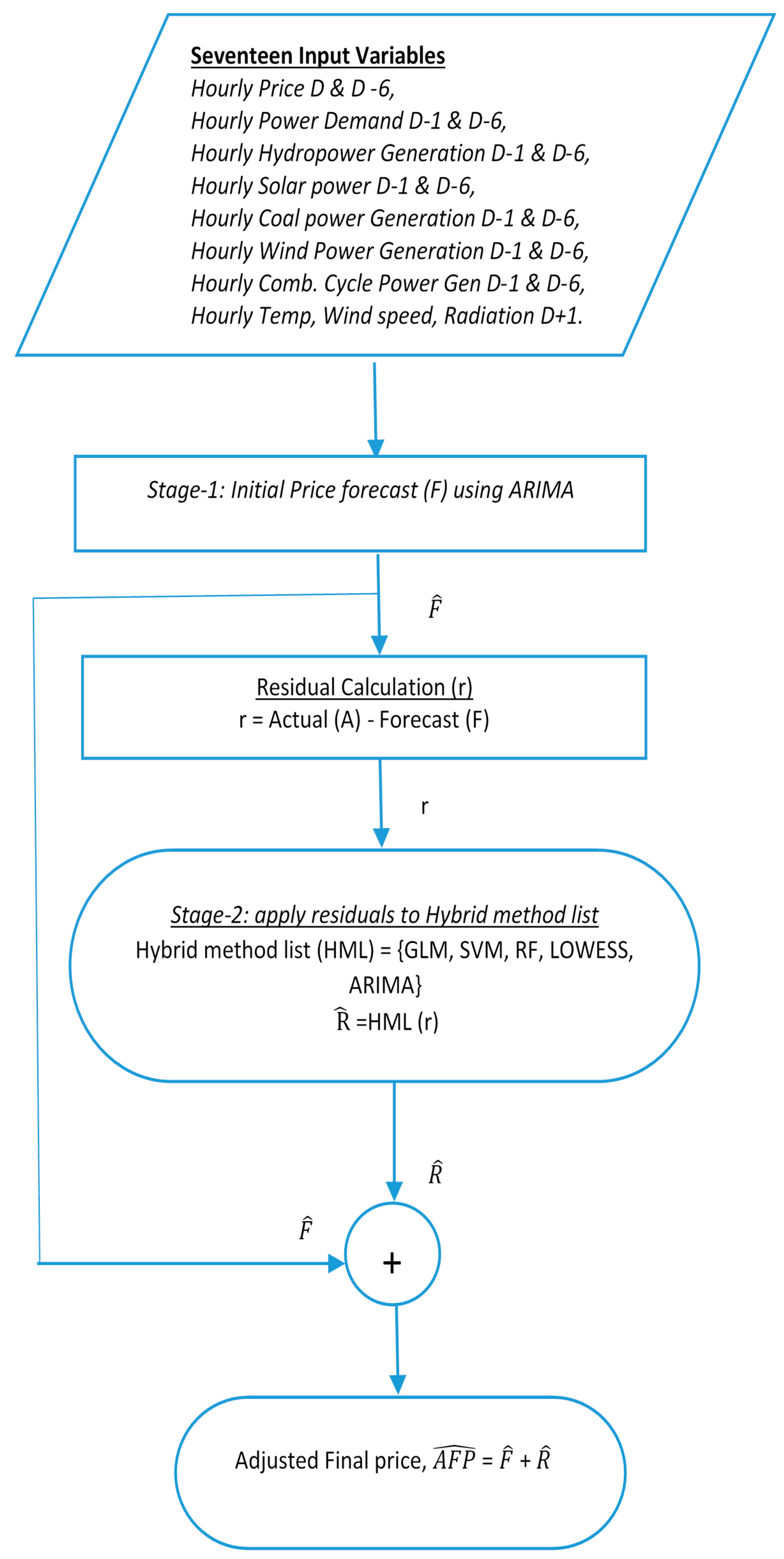
The Flowchart in
Figure 1 shows that the initial price forecast is carried out by ARIMA deployed in Stage-1 and residuals are then computed before Stage-2 begins. In Stage-2, residuals are fed as input to the collection of other forecasting methods. The two-step residual extraction method has been briefly reported using ARIMA with GLM in our previous paper [
38]. In the present paper, we are applying the same process to ARIMA-SVM, ARIMA-RF, ARIMA-LOWESS and ARIMA-ARIMA. Some details on the proposed two-stage model are provided next.
This two-stage approach was proposed to improve the forecasting estimation that mutually benefits from ARIMA and the other methods. In this approach, ARIMA was considered in the first stage since it is a well-known stochastic process known for performing well with the time series dataset. This process was executed in R Programming environment. In the first stage, a dataset containing all the 17 predictor variables such as hourly price, demand, generation and temperature variables were used to build an ARIMA model. To build this model, a statistical package known as ‘arima’ was used. This ARIMA model was used to predict the price (F) for the day-ahead electricity market. Residual dataset (r) is created by differencing the forecasted values (F) from the actual values (A).
In the second stage, the residual dataset (r) is fed as a time-series dataset to the different methods. In this case, methods such as GLM, SVM, RF, LOWESS and ARIMA. Future residuals (R) are predicted using all these methods. This future residual (R) are added along with the forecasted price (F) from the ARIMA model in the first stage to get the final adjusted price (AFP). The details of the first and second stage approach are given in the next sub-section.
Table 1 demonstrates the combination of the ARIMA model (p, d, q) with the MAPE values for the different duration of the datasets.
3.1. Stage-1: Initial Price Forecast (F) Using ARIMA
Step 1. In Stage-1, ARIMA was used to predict the day-ahead prices. Input variables that are considered include historical electricity prices, generation and consumption load and weather data like solar irradiance, temperature and wind speed. These variables are fed as time-series data to the ARIMA model. The relationship between the predictor variables and forecasted variables is then initialized through this model.
Step 2. An ‘auto-arima’ function built in R-software was used to identify the best-fit by inputting the residual values (p, d, q) of the three-time series components I, AR and MA. After identifying the best-fit model, the ‘forecast’ function is used to predict the day-ahead price.
Step 3. The same process is repeated for other datasets. In this study, one week, two weeks, three weeks, one month, 45 days, 60 days and 75 days of datasets from the Iberian electricity price market are used to predict the day-ahead electricity prices.
Step 4. After the price predictions, residuals are calculated by differencing the predicted value (f) from the actual value (A).
3.2. Stage-1: Input Residuals to the Hybrid Model
3.2.1. ARIMA-SVM
The steps involved in the two-stage residual extraction method, that uses combinations of ARIMA and SVM, are as follows:
Step 1. In Stage-2, the residual dataset is fed as an input to the SVM model. SVM model is then initialized by calling the function ‘ksvm’ which is available in the kernlab package. The SVM model is then used to predict the residual for the next day by calling the ‘predict’ function.
Step 2. Finally, the calculated residual (R) from Step 1 is then added to the predicted price from the ARIMA method (P) to get the final price.
3.2.2. ARIMA-RF
The following are the steps in deploying the hybrid combination of ARIMA and RF methods to forecast the day-ahead price:
Step 1. In Stage-2 of the hybrid model, the residuals from the ARIMA model are fed as time series input data to the RF model. The ‘random forest’ function in the Random Forest package of R helps in fitting the RF model.
Step 2. The RF model is then used to predict the future residuals (R) which are added to the earlier predictions to obtain the adjusted final price forecast.
3.2.3. ARIMA-LOWESS
The following are the steps in deploying the hybrid combination of ARIMA and LOWESS methods to forecast the day-ahead prices:
Step 1. In the Stage-2 of the hybrid model, the residual dataset from the ARIMA model is fed as time series input data to the LOWESS model. The ‘loess’ function in the Stats package of R helps in fitting the LOWESS model.
Step 2. The loess model is then used to predict the future residual (R) which is added along with the predicted price to get the final price forecast.
3.2.4. ARIMA-ARIMA
The following are the steps in deploying the combination of ARIMA and ARIMA to forecast the day-ahead price:
Step 1. In Stage-2 of the hybrid model, the residuals from the ARIMA model are fed as input data to the same ARIMA model. The ‘auto-arima’ function in the Stats package of R helps in fitting the ARIMA model in Stage-2.
Step 2. The ARIMA model is then used to predict the future residual (R) which is added along with the predicted price from the ARIMA method in the first stage to get the final price forecast.
5. Results and Discussion
As discussed above, several two-stage hybrid models have been used to predict the electricity prices of the Iberian Markets in this study. The hybrid models include ARIMA-GLM, ARIMA-RF, ARIMA-SVM, GLM and ARIMA-LOWESS. The hybrid models are trained and tested using datasets ranging from one-week to three months.
The dataset durations include one-week, two-weeks, three-weeks, one month, 45 days, 60 days, 75 days and 90 days. The specific data durations are shown in
Table 3. We evaluate the performance of our forecast models through a statistical measure known as MAPE (Mean Average Percentage Error) which represents the daily error in price predictions.
Table 3 shows a numerical comparison of the MAPE values for various data durations.
Figure 2,
Figure 3,
Figure 4,
Figure 5,
Figure 6,
Figure 7 and
Figure 8 graphically show the MAPE comparison of hybrid models. Each figure shows the MAPE comparison of ARIMA, ARIMA-GLM, ARIMA-RF and ARIMA-SVM. All the variables have been taken into consideration.
However, in
Figure 9, only four variables are considered since LOWESS can be modeled only with a maximum of four variables. In the last dataset (90 days), all methods use the following specific four variables: Price D, Price D-6, Power demand D-1 and Power demand D-6.
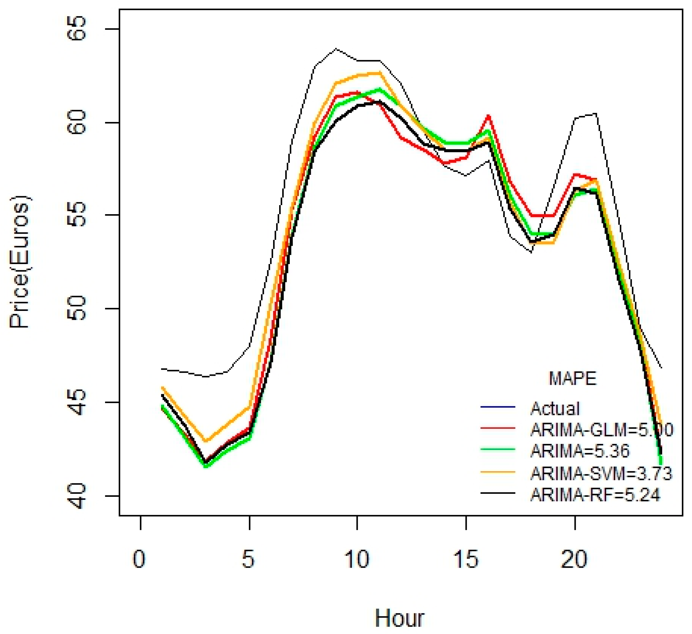
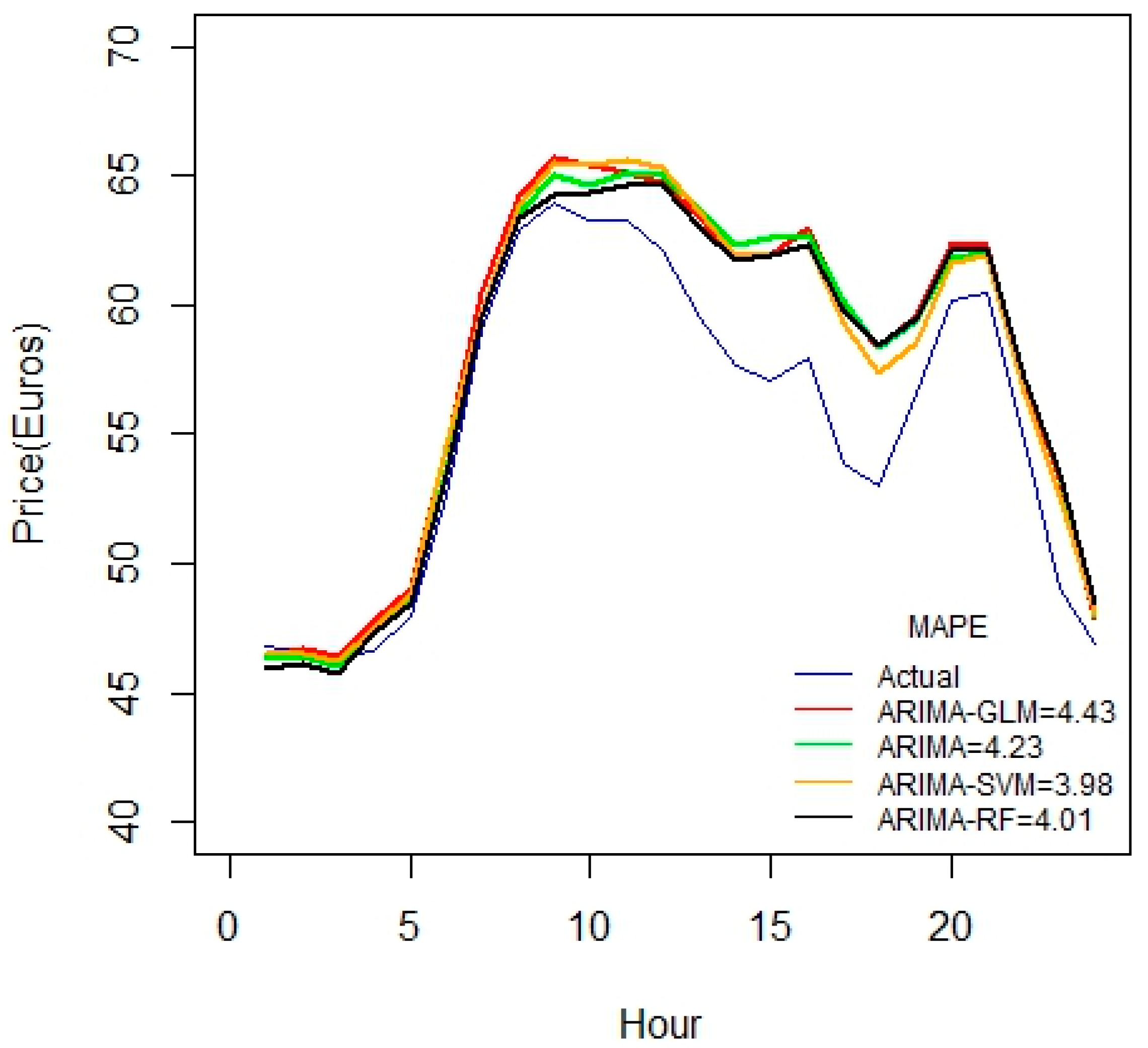
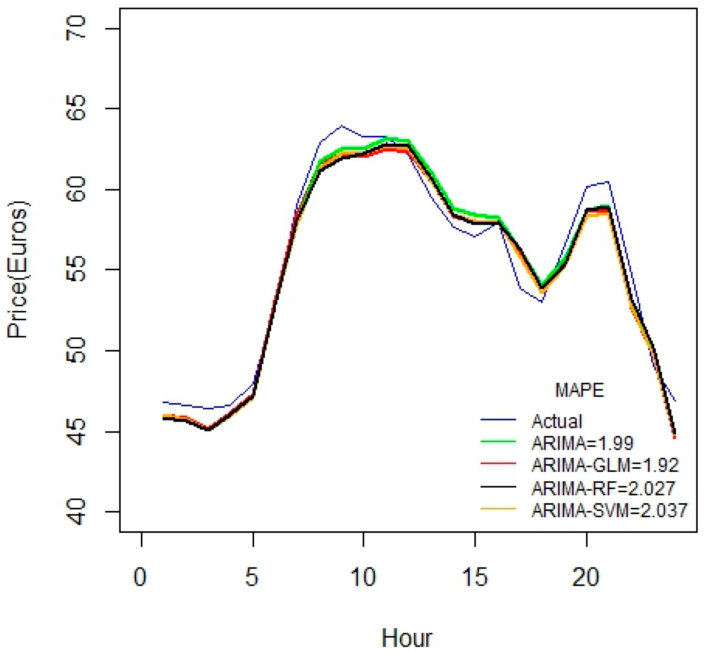
Figure 2 indicates that ARIMA-SVM combination outperforms other methods using a one-week dataset. In addition, from
Table 2 it is also evident that the ARIMA-SVM model gives a better prediction with smaller durations of data such as for one week, two weeks, three weeks and one month.
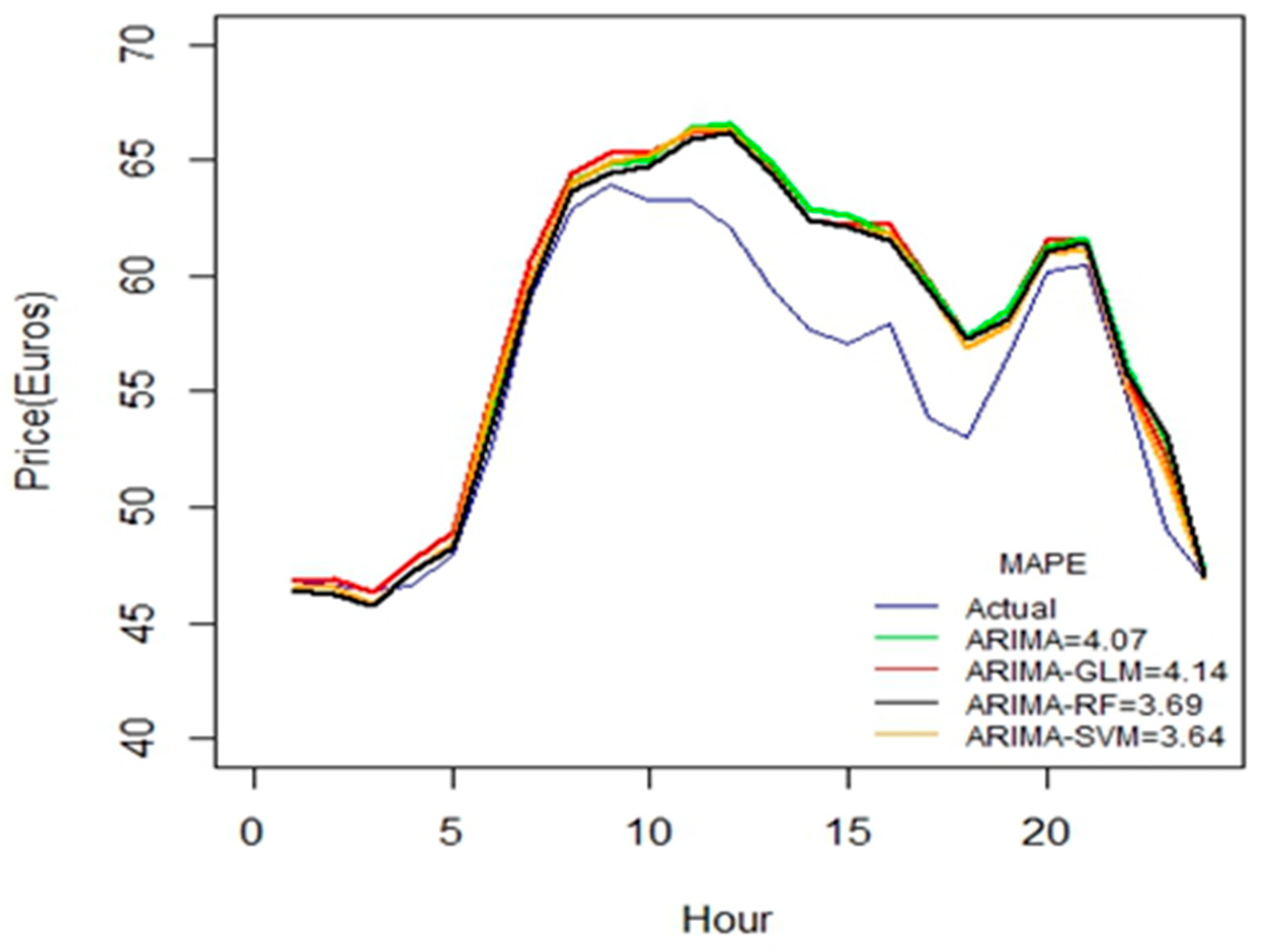
From
Figure 3, we observe that MAPE values for two weeks are reduced but not substantially. One of our objectives was to test multiple durations of the datasets and observe how MAPE changes with the duration of datasets.
From
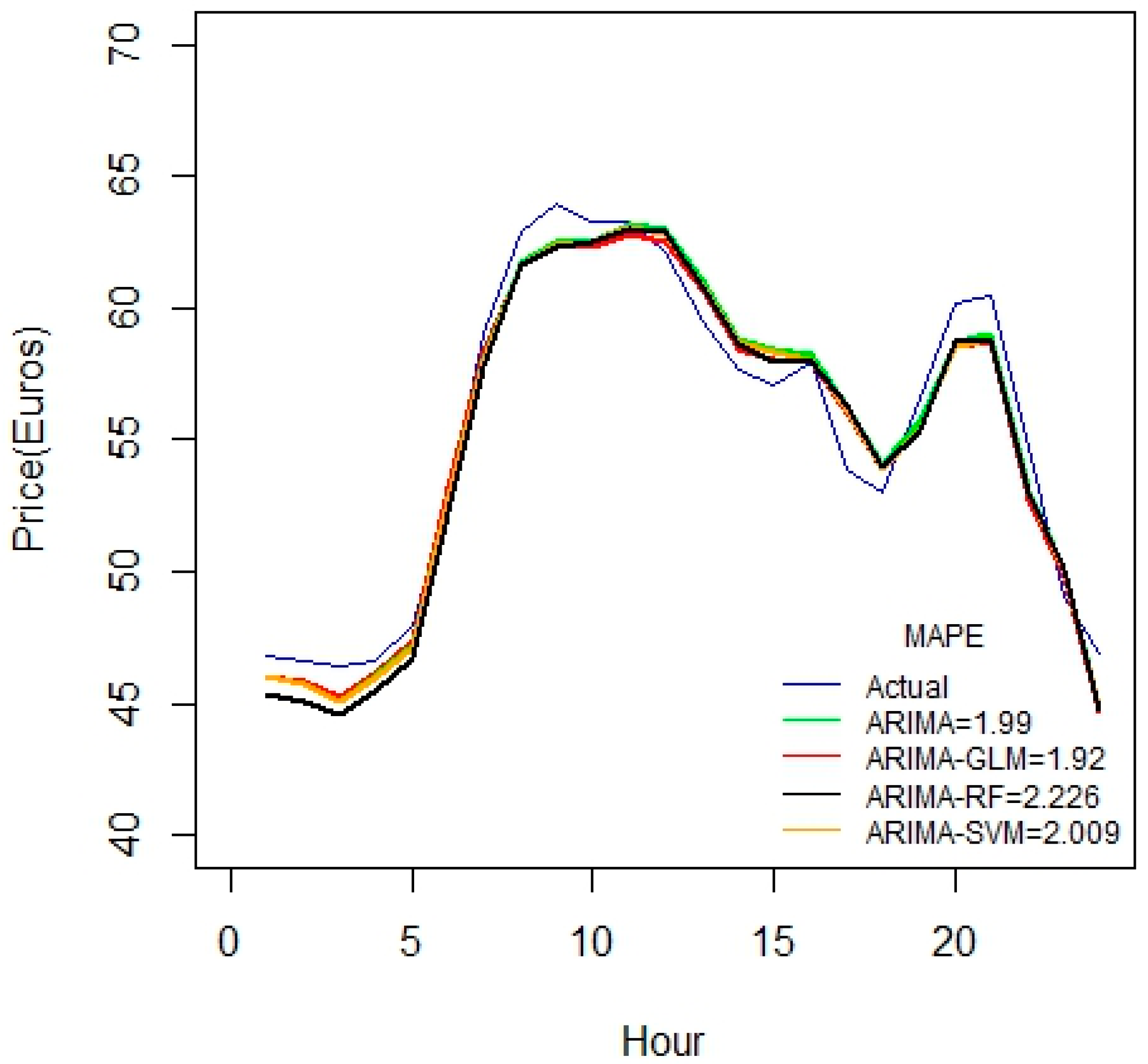
Figure 4, it is yet again evident that the combination of ARIMA-SVM performs better than other methods with 17 variables.
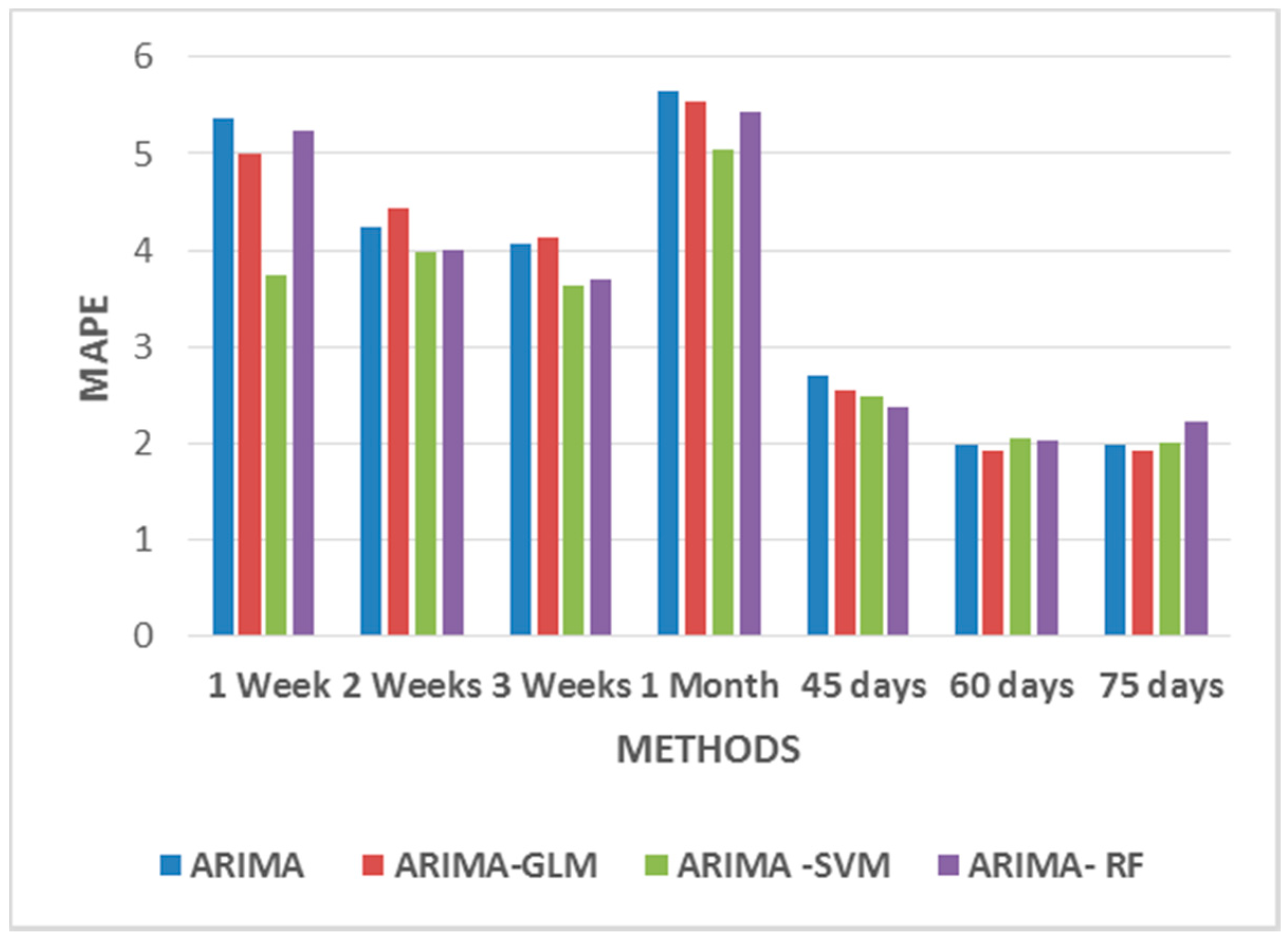
From above, it is noted that the MAPE values are reduced as the duration of the datasets is increased. Using 17 variables in the above case studies, there seems to be a linear reduction in MAPE values starting from one to three weeks. Another important inference from these results is that there is a sharp reduction in MAPE for ARIMA-RF combination than other methods. This is a strong evidence that the random forest is well-suited for larger datasets.
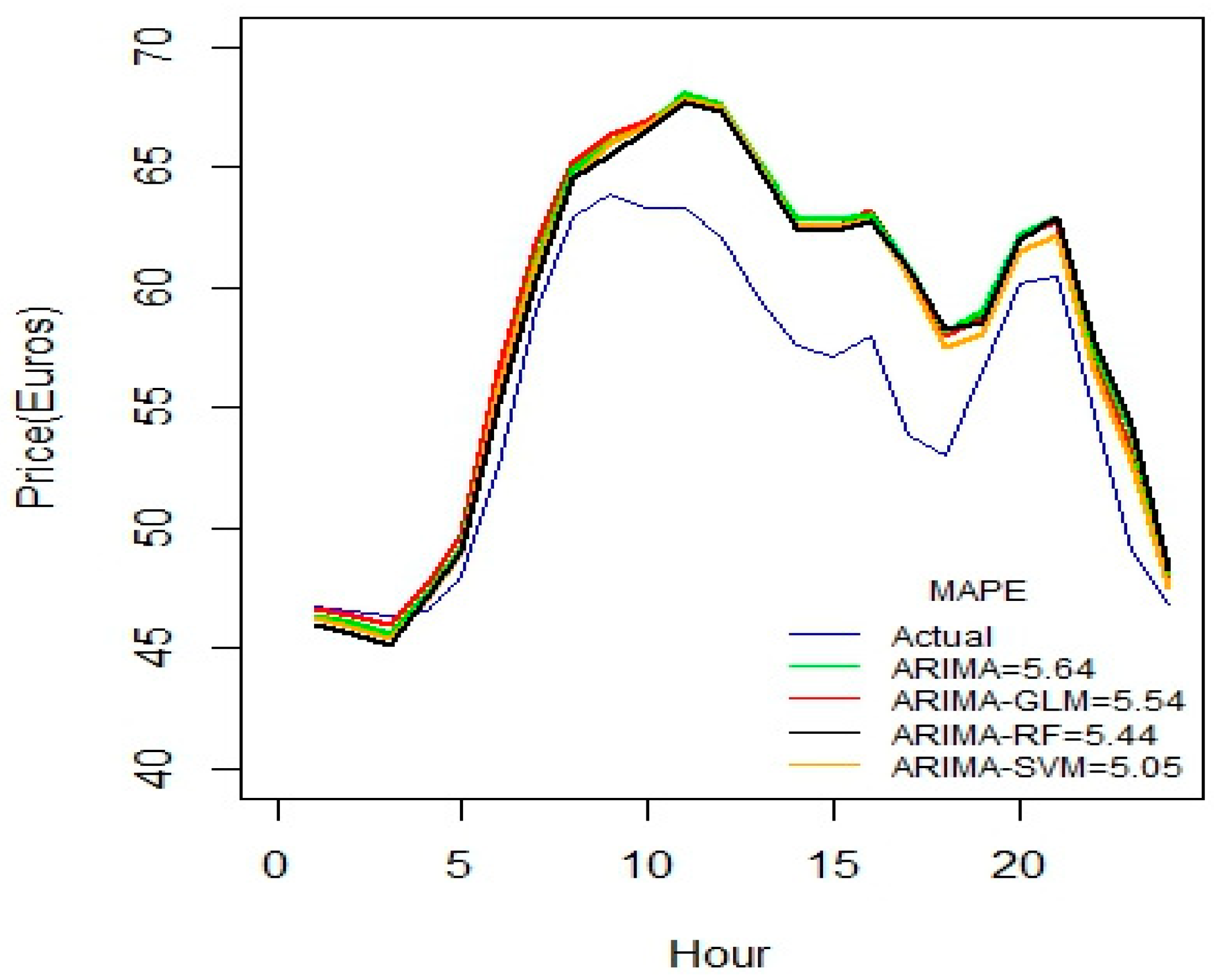
For the 1-month duration of data seen in
Figure 5, error values seem to increase compared to the 3-week data set. This may be due to some irrelevancy or missing fields in data. This might also due to the fact that the price variable is not highly correlated with the predictor variables.
From
Figure 6, the accuracy of the calculated values has improved when substantially considering all the seventeen variables. If one includes the important variables such as price D and price D-6, one can then greatly reduce the forecasting error. We find that the ARIMA-RF is effective for larger datasets, because the ensembles take a small portion of the dataset.
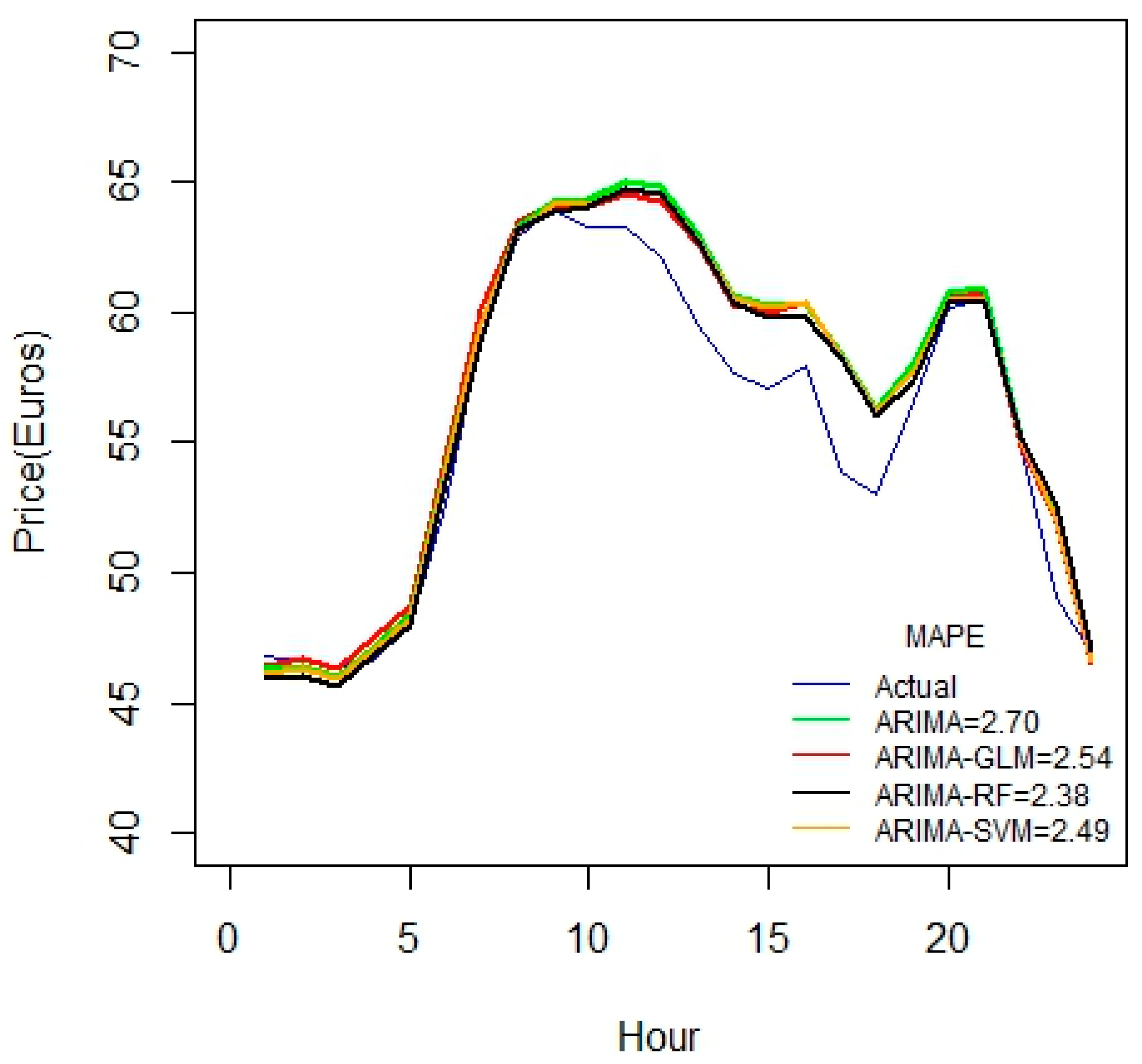
As seen from
Figure 7, these hybrid models work better for durations greater than 45 days. All the proposed hybrid combinations closely predict the pattern of price-spikes, while matching with the actual data.
A similar conclusion can be inferred from
Figure 8, as the duration of datasets increases.
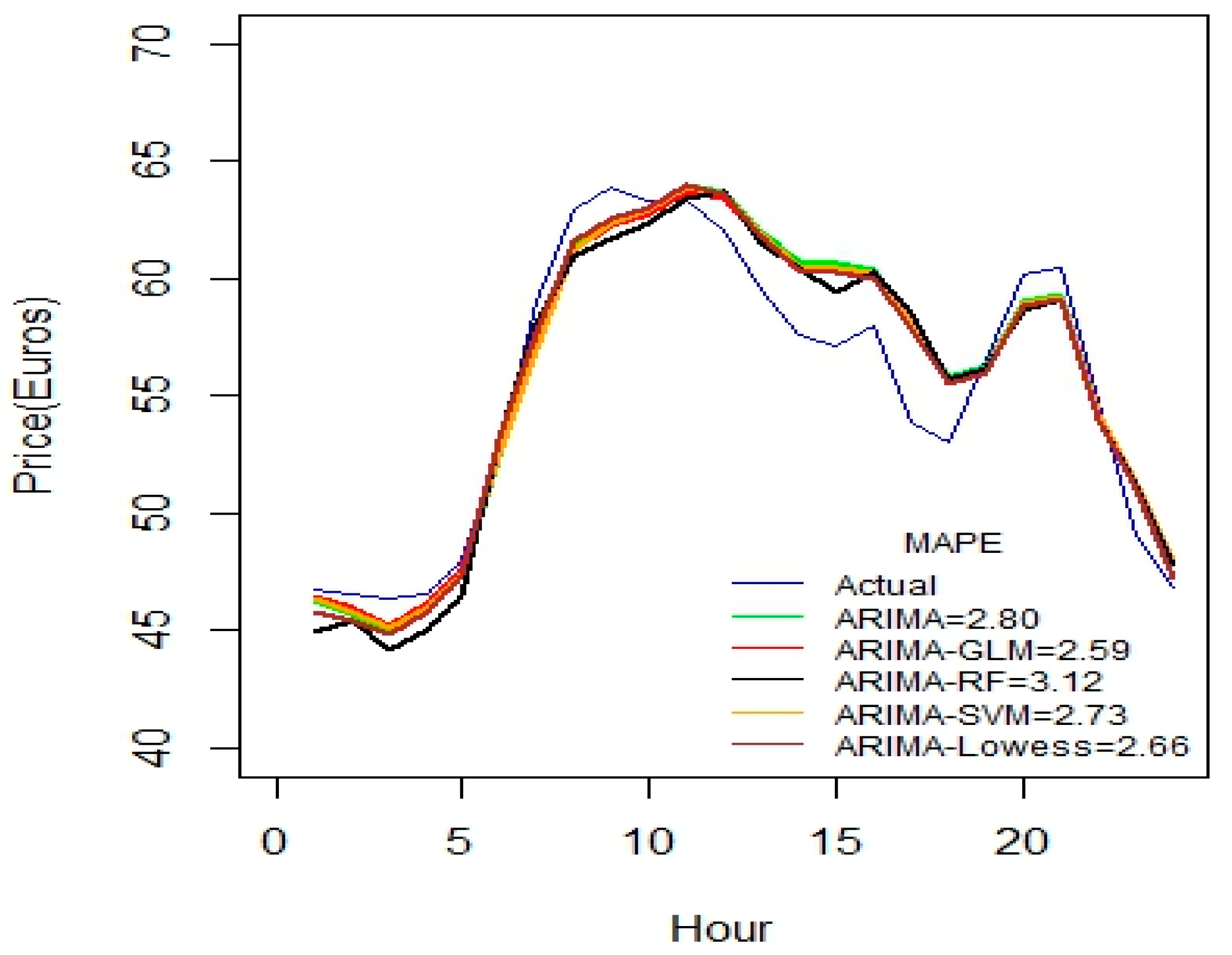
Table 4 shows the MAPE results for the 90 days dataset using four variables (Hourly Price D, Hourly Price D-6, Hourly Power Demand D-1 and D-6). Since LOWESS cannot be used with more than four variables, the ARIMA-LOWESS model is compared with the other hybrid models also using the same four variables as shown in
Figure 9.
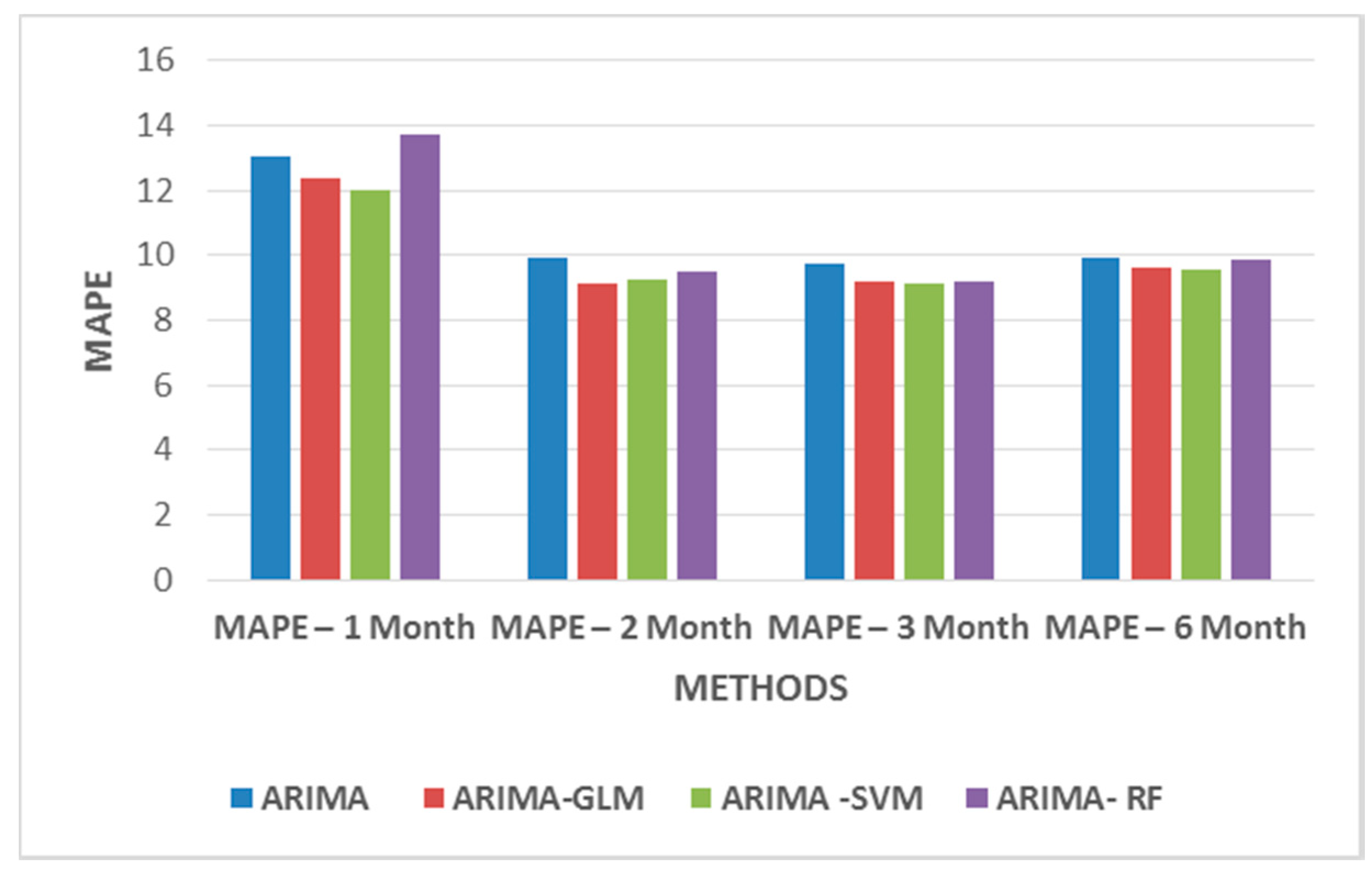
Figure 10 compares the MAPE values from one-week to 75 days. From
Figure 10, it can be seen that the models may need to be tested with additional data durations for scalability. For such models, variables such as price, load and temperature values have been considered. The MAPE error can be significantly reduced by considering only those important variables that highly correlate with the price.
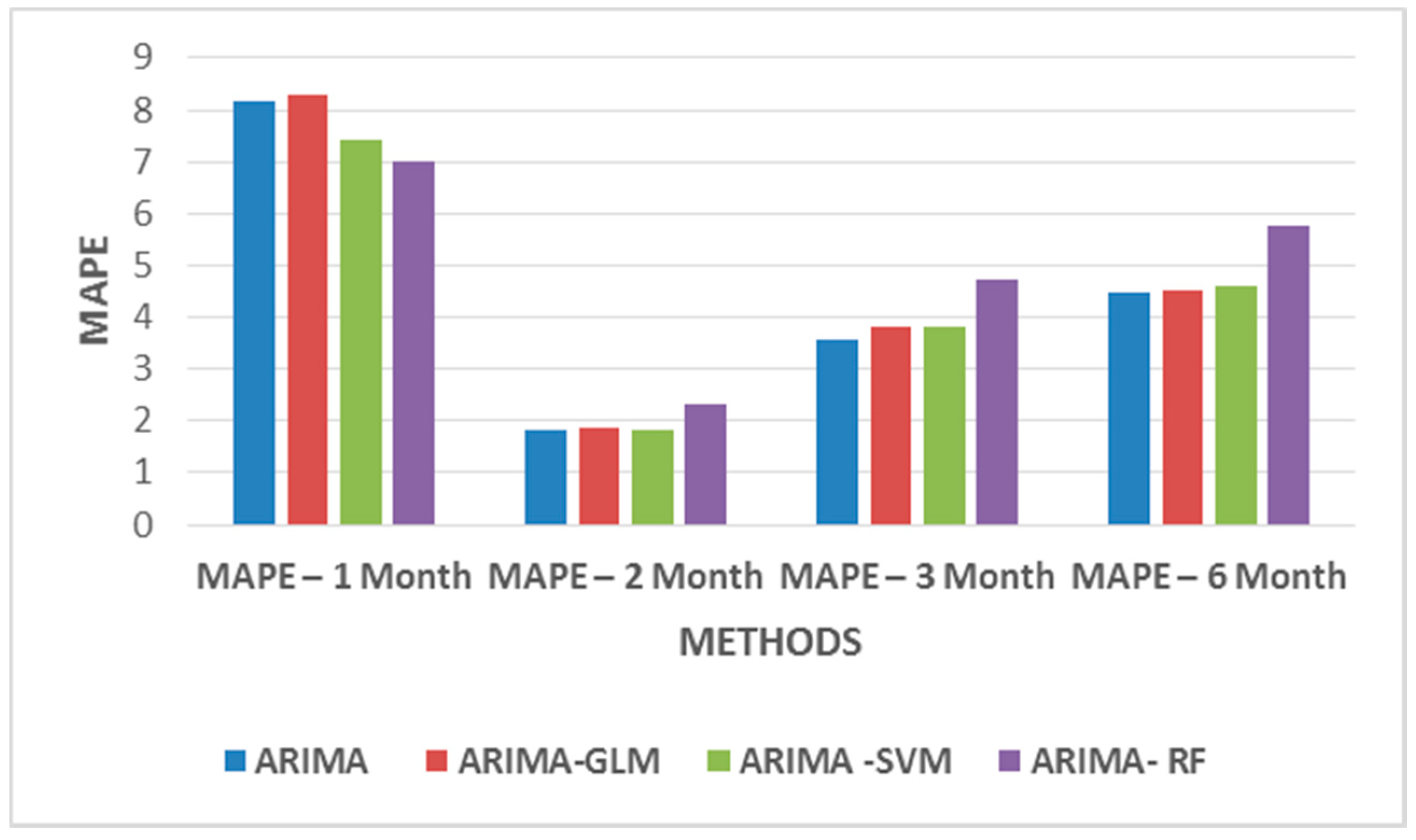
The electricity market has to be studied thoroughly to consider which variable significantly impacts the electricity price. The larger penetration of renewable energy sources such as wind and solar resources into the grid might impact the price significantly. The weekday and weekend patterns were also analyzed using our proposed model and the results are summarized in
Table 5 and
Table 6.
From
Table 5, one infers that two months of weekday datasets give a better prediction, as this dataset highly correlates with the predicted price. For weekend datasets, only 10 variables are considered to be of importance. The variables that take previous day’s influence into consideration were removed from the datasets. Thus, taking into consideration only variables such as hourly price D-6, hourly power demand D-6, hourly hydropower generation D-6, hourly solar power D-6, hourly coal power generation D-6, hourly wind power generation D-6, hourly combined cycle power generation D-6, temp, wind speed, radiation D+1, etc.
Figure 11 and
Figure 12 show MAPE values for weekday and weekend datasets. The results do not significantly improve the MAPE values but they certainly indicate that the models may require additional data to identify patterns for better forecasts.
Table 7 shows the MAPE results for the two-stage ARIMA models with and without explanatory variables in the Stage-2. From these results, one can clearly infer that the inclusion of the explanatory variables in Stage-2 has great influence on the residual predictions.
Table 8 presents and compares the MAPE results of the Iberian electricity market as published in the literature. This comparative table clearly strengthens the fact that the ARIMA–based two-stage model is a promising forecasting method to improve the accuracies in residual training for short-term price forecasting.
Table 9 categorizes the MAPE results as good, average and bad for easy classification of readers. MAPE results between 1–4.99% are termed as good results, while MAPE results between 5–9.99% is classified as average results. MAPE results above 10% are classified as poor results. One can infer that the MAPE results are good for most of the data duration except for one week and one month.
Table 10 shows the statistical test results conducted for different methods for the different duration of the Iberian electricity market. Correlation test was conducted to identify the statistical significance and to find out which method was superior to the other. This provides insights into the strength of the linear association between the forecasted and the actual value.
Correlations close to 1 indicates a very strong linear relationship between the two variables. Therefore, the correlation here of about 0.9 indicates a strong relationship for all the hybrid models for all the different dataset.
The results show that the ARIMA-SVM method outperformed other hybrid models for smaller dataset such as one week and two weeks, while for larger dataset ARIMA-GLM showed superiority than the other hybrid models.


 ,
, 


