Article

Score Cloud Analysis for Rule-Aware Ranking Robustness Under Discrete Judgment Uncertainty

by
Sebastiano Ettore Spoto
Federazione Italiana Wushu Kung Fu e Arti Marziali Vietnamite (FIWuK), 00135 Roma, Italy
Stats 2026, 9(5), 87; https://doi.org/10.3390/stats9050087
Submission received: 8 July 2026 / Revised: 20 August 2026 / Accepted: 21 August 2026 / Published: 24 August 2026

Abstract

Rule-defined rankings often transform continuous marks, discrete judgments, trimming rules, caps, truncation, and tie-breaking variables into a single official order. When ranking margins are small, a formally valid outcome may nevertheless be sensitive to marginal changes in the recorded decision state. This article presents Score Cloud Analysis as a rule-aware statistical sensitivity-reporting method for such systems. The method represents the official score as a deterministic function of recorded inputs and recomputes scores and ranks under finite perturbations, rather than relying on local linear approximations. It defines deterministic diagnostics, including directional Group A/Group C (A/C) decision exposures and their aggregate contested-point exposure, total sensitivity exposure, fragility-to-margin ratios, Score Cloud overlap, and single-call rank sensitivity, and separates these from scenario-conditional Monte Carlo Rank Cloud frequencies. The method is illustrated using a synthetic Wushu Taolu case study because that setting contains majority decisions, trimmed rater marks, discrete difficulty values, Head Judge adjustments, and tie-break rules. The synthetic experiment is an internal-consistency stress test, not an empirical validation and not an estimate of judging-error rates. A small sensitivity study varies perturbation scale and intra-athlete dependence to show which conclusions are scenario-specific. The method separates procedural validity from local rank robustness and is transferable to other reconstructable, rule-based, rater-mediated ranking systems.

1. Introduction

Rankings are often reported as if they were simple orderings of observed quantities. In many applied settings, however, the reported order is generated by a rule-defined scoring procedure. The score may combine continuous marks, binary or categorical judgments, trimming rules, caps, truncation conventions, and tie-breaking variables. In such systems, the official result can be perfectly valid under the rule while the local ordering remains sensitive to small changes in recorded decision states. The statistical problem is therefore not only how to compute the official score, but also how to report whether the induced ranking is stable under explicitly specified perturbations.
A minimal example makes the operational question concrete. Consider two athletes separated by only 0.003 points. If one recorded 2–1 decision in Group A or Group C (A/C) is reversed, the resulting score change may equal or exceed that official margin. Full score recomputation can then produce a score tie or inversion, after which the official tie-break chain must also be recomputed. The recorded result can remain procedurally valid while its local stability is limited; Score Cloud Analysis is designed to report that distinction.
This problem appears in league tables, educational accountability systems, clinical composite scores, grant panels, rater-mediated assessments, and judged sports. Previous statistical work has discussed uncertainty in institutional rankings and league tables [1,2], uncertainty and sensitivity analysis for composite-indicator rankings [3], global and local sensitivity analysis [4,5], uncertainty propagation [6,7], rater reliability and generalizability [8,9,10,11,12], judged-sport rater behavior [13,14], and robustness of estimators under contamination [15,16]. The present article does not replace these studies. It links them to a narrower reporting problem: how to diagnose local rank sensitivity when the ranking is generated by a known nonlinear rule containing discrete decisions and ordered statistics.
Modern Wushu Taolu is used as a synthetic case study because its rulebook offers a compact example of a nonlinear, rater-mediated scoring grammar. The 2024 International Wushu Federation rules define events with Degree of Difficulty using Quality of Movements, Overall Performance, and Degree of Difficulty components, and events without Degree of Difficulty, including Duilian and Jiti, using Quality of Movements and Overall Performance [17,18]. The rules include majority decisions, a five-mark trimmed Overall Performance component, Head Judge adjustments, and event-specific tie-breaks. These features make the setting useful for testing a rule-aware sensitivity-reporting method. The manuscript does not analyze any empirical competition result.
The method proposed here is called Score Cloud Analysis. It treats the official score as the output of a deterministic rule function, then studies finite perturbations of selected input states. The key distinction is between procedural validity and rank robustness. Procedural validity answers who wins under the rule. Rank robustness asks how stable that ordering is under declared perturbations of marginal calls, retained marks, adjustment terms, or tie-break variables.
This distinction is deliberately modest. A ranking can be locally robust under the recorded rule and still be biased relative to an unobserved true performance order if all recorded evaluations share a systematic error. Conversely, a ranking can be locally sensitive even when the recorded calls are substantively correct. Score Cloud Analysis estimates neither true athletic merit nor empirical rater error. It reports sensitivity of the official ranking rule under explicit deterministic or probabilistic perturbation assumptions.
Figure 1 summarizes the analytical sequence. The official record is transformed by a score function and a ranking function. Deterministic diagnostics describe score and rank sensitivity from recorded marginal states. Scenario-conditional perturbation models add weights to perturbation states and produce Monte Carlo Rank Cloud frequencies. Empirical calibration would require independent review or repeated panels.
Table 1 positions the proposed reporting method relative to adjacent statistical approaches and makes explicit which elements are retained from existing methods and which reporting objects are added here.
Table 2 records the main claims and non-claims. These boundaries are central to the interpretation of the synthetic experiment.

2. Materials and Methods

2.1. Structural Representation of a Rule-Defined Ranking

Let competitors be indexed by i = 1 , , n . The observed record for competitor i is denoted
x i = ( z i A C , b i , h i , t i , q i ) ,
where z i A C denotes discrete A/C decision states, b i denotes rater marks, h i denotes rule-based adjustment states, t i denotes tie-break variables, and  q i contains other rule-defined quantities. The official score is represented as
s i = f R ( x i ) ,
where R is the rulebook. The official ranking is then
r = ρ R ( s , t ) ,
where s = ( s 1 , , s n ) is the score vector, t contains the rule-defined tie-break variables, f R is the score map, and  ρ R is the ranking map. Equations (2) and (3) are deterministic. Randomness enters only when the analyst assigns a distribution to perturbation states.
This representation is compatible with structural counterfactual notation, but it does not identify causal effects. Structural causal models use deterministic assignments together with uncertainty over some determinants [19,20]; here, selected recorded components are replaced and the deterministic rule is recomputed. The perturbations therefore define rule counterfactuals rather than identified causal effects.
Let ω i denote a perturbation state:
ω i = ( z i A C , , b i , h i , t i ) .
The perturbed input is x i ( ω i ) and the recomputed score is
s i ( ω i ) = f R ( x i ( ω i ) ) .
For a pair ( i , j ) , the recomputed ranking is
r ( ω ) = ρ R ( s ( ω ) , t ( ω ) ) .
This formulation avoids a linear-additive assumption. Additive decompositions may be used as screening summaries, but the operative computation is the rule-aware recomputation in Equations (5) and (6).

2.2. Wushu Taolu as a Synthetic Case Study

In the synthetic case study, the official score has the schematic form
s i = τ 3 ( A i + B i + C i H i + G i ) ,
where A i is the quality or execution component, B i is the Overall Performance component, C i is the Degree of Difficulty component when applicable, H i is a signed Head Judge deduction term expressed as a subtraction, G i is a bonus or adjustment term when present, and  τ 3 denotes the three-decimal truncation operator used in the synthetic reporting layer. Real applications must follow the event-specific official reporting rule.
The Overall Performance component is calculated from five displayed marks. If 
b i ( 1 ) b i ( 2 ) b i ( 3 ) b i ( 4 ) b i ( 5 ) ,
then
B i = τ 3 b i ( 2 ) + b i ( 3 ) + b i ( 4 ) 3 .
The lower discarded mark is
B i L D = b i ( 1 ) .
This quantity is excluded from the B-score estimator in Equation (9) but may re-enter the official ranking function as a tie-break variable in events where the rulebook specifies it. Thus, full reconstruction of tied-score ranking requires the five-mark vector, not only the trimmed mean. Supplementary File S1 gives the event-specific rule details and the treatment of residual official ex aequo.
For the synthetic output files, a final athlete identifier may be used only to sort rows deterministically in comma-separated values (CSV) tables. It is not part of ρ R and has no sporting interpretation.

2.3. Deterministic Score-Cloud Diagnostics

A marginal A/C decision is a recorded decision state whose outcome would change if one member of the three-judge group changed vote. For example, under a two-out-of-three threshold, 2–1 and 1–2 states are one-vote reversible. Let M i be the set of marginal A/C decisions for competitor i. Each decision M i has a signed finite-difference effect
δ i = f R ( x i ( ) ) f R ( x i ) ,
where x i ( ) differs from x i only by the specified rule-counterfactual reversal of decision .
Directional A/C exposure is defined as
E i = M i max { δ i , 0 } , E i + = M i max { δ i , 0 } ,
with aggregate contested-point exposure (CPE)
CPE i A C = E i + E i + .
The exact Score Cloud is defined first as the image of the admissible perturbation set,
C i exact = { f R ( x i ( ω i ) ) : ω i Ω i } ,
with exact min–max hull
H i exact = min c C i exact c , max c C i exact c .
A separate additive screening envelope is used when one-at-a-time finite differences are summarized without exhaustive joint enumeration. For A/C calls alone,
E i A C , scr = [ s i E i , s i + E i + ] .
This envelope is not called exact unless the admissible perturbations are jointly additive and interaction-free under the rule. For  | M i | binary A/C decisions, exhaustive enumeration may scale as 2 | M i | . Monte Carlo sampling is a computational approximation to weighted enumeration when the perturbation space is large or when scenario weights are assigned.
For adjacent pair ( i , j ) with official leader i, define the official margin
Δ i j = s i s j .
The raw A/C fragility-to-margin ratio (FMR) is
FMR i j A C = E i + E j + | Δ i j | , Δ i j 0 .
When Δ i j = 0 , the raw ratio is undefined and the pair is tie-break active. For plotting or screening only, an epsilon-regularized value may be computed as
FMR i j A C , ε = E i + E j + max ( | Δ i j | , ε ) .
For the synthetic implementation, the deterministic B screening half-width is the declared quantity
U B , i scr = u B , i 0 .
The value u B , i is pre-specified by the synthetic B variation profile and reported as B_block_halfwidth in Supplementary File S2: 0.019 for low-variation profiles, 0.030 for moderate-variation profiles, and 0.055–0.070 for high-variation profiles. It is independent of the Gaussian Monte Carlo scale and is neither a distributional quantile nor a confidence limit. If  d H , i is the signed total-score change when the Head Judge perturbation state is activated, define directional terms
U H , i = max ( d H , i , 0 ) , U H , i + = max ( d H , i , 0 ) .
The total athlete-level screening interval displayed in Figure 2 is therefore
E i tot , scr = s i E i U B , i scr U H , i , s i + E i + + U B , i scr + U H , i + .
For an adjacent official leader i and follower j, screening contact is declared when the leader’s lower endpoint is no greater than the follower’s upper endpoint; equality is recorded separately as tie activation. The corresponding total sensitivity exposure (TSE) is
TSE i j = E i + E j + + U B , i scr + U B , j scr + U H , i + U H , j + .
The total epsilon-screened fragility-to-margin ratio is
FMR i j tot , ε = TSE i j max ( | Δ i j | , ε ) .
The synthetic study uses ε = 0.001 score units, matching the public three-decimal reporting grid. Recomputing the synthetic labels with ε { 0.0005 , 0.001 , 0.002 , 0.005 } leaves the baseline red/amber/green pair counts unchanged (11/10/8). Total FMR is interpreted only as a screening ratio, not as a probability.
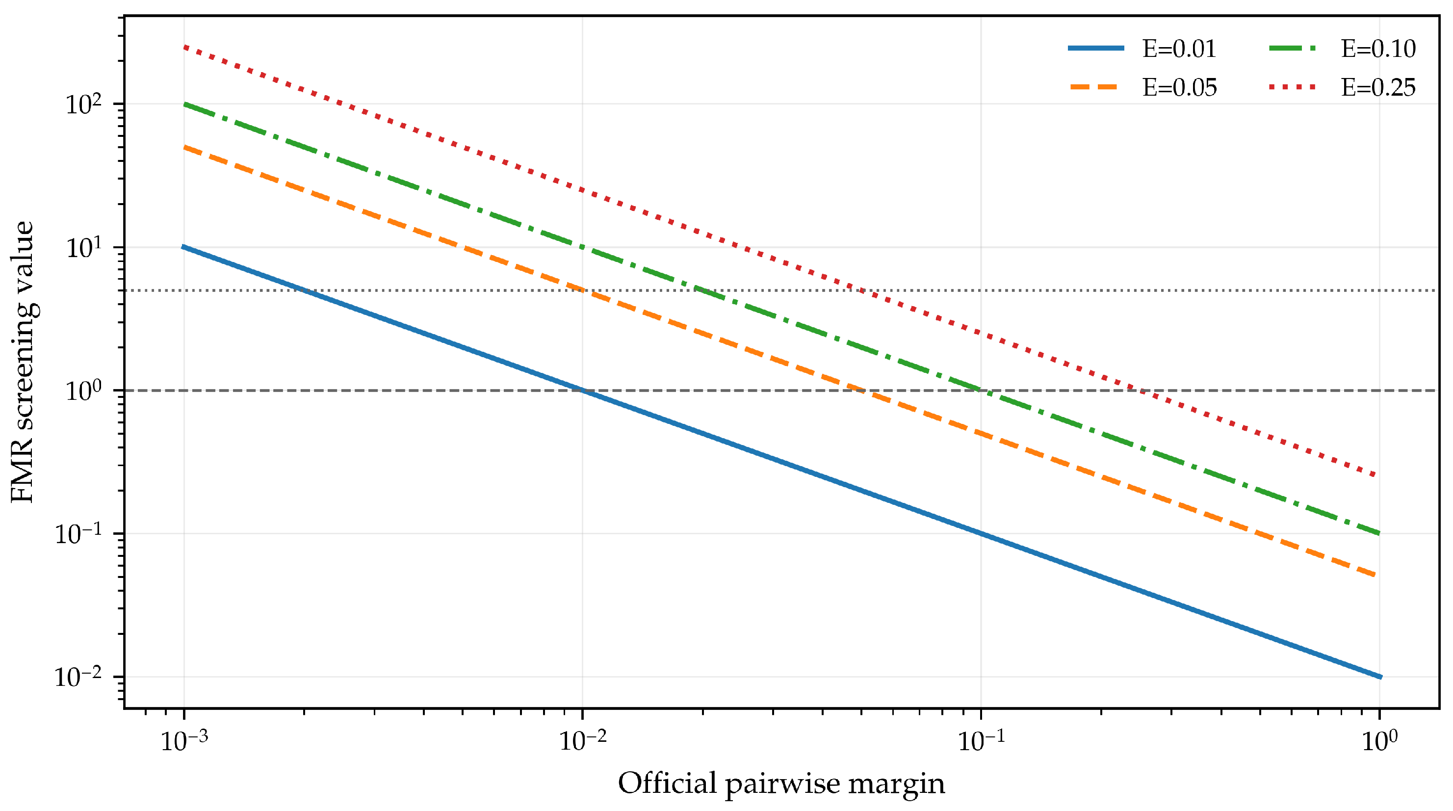
Figure 3 shows why FMR must be interpreted with caution near zero margins. The statistic is informative as a normalized screening value, but it is undefined at exact zero margin and can become very large for millipoint-scale separations.
Figure 3. Fragility-to-margin ratio (FMR) as a function of official pairwise margin for several fixed exposure levels. Dashed horizontal reference lines at FMR = 1 and FMR = 5 are the synthetic screening thresholds used in Table 3; they are illustrative, not empirically validated cut-points. The figure also shows the instability of raw ratios near zero margins.
Stats 09 00087 g003
Table 3. Synthetic adjacent-pair screening labels used in the stress test. The rules are declared conventions for the artificial examples only. A/C denotes Group A/Group C decisions.
LabelSynthetic Rule
RedAt least one of the following holds: π ^ i j R , inv 0.20 ; FMR i j tot , ε 5 ; A/C single-call tie/rank activity is present; or the official score margin is zero.
AmberThe pair is not red, and at least one of the following holds: π ^ i j R , inv 0.05 ; FMR i j tot , ε 1 ; or deterministic screening envelope overlap/tie activity
is present.
GreenNeither the red nor the amber condition holds under the declared synthetic screening convention.

2.4. Single-Call Rank Sensitivity

A pair is A/C single-call active when changing one marginal A/C decision is sufficient to produce a score inversion, a score tie, or tie-break activation under the official ranking rule. Let
L i j = max { max M i ( δ i ) + , max M j ( δ j ) + } .
The pair is single-call rank active if
L i j Δ i j
on the official reporting grid. Equality is important because a score tie can activate official tie-breaks.

2.5. Group B Sensitivity and Discarded Mark Re-Entry

Before display quantization, a single retained-mark perturbation of + 0.01 changes the retained three-mark mean by
Δ B ¯ ret = 0.01 3 = 0.003 3 ¯ ,
provided that the retained set is unchanged. After applying τ 3 , the displayed change is instead
Δ B disp = τ 3 ( B ¯ ret + 0.01 / 3 ) τ 3 ( B ¯ ret ) ,
and need not equal 0.003 3 ¯ exactly. Likewise, a common-mode + 0.01 shift in all three retained marks produces an unquantized retained-mean change of 0.01 , while the displayed change remains subject to the reporting operator. If retained-mark perturbations have common variance σ B 2 and pairwise correlation ρ , the retained-block surrogate, before quantization, re-ordering, re-trimming, and truncation, has
σ B , eff 2 = σ B 2 3 ( 1 + 2 ρ ) .
The mark-level synthetic baseline perturbs all five displayed B marks, returns them to the two-decimal grid, orders them, trims them, recomputes B i , recomputes B i L D , and then recomputes ρ R . The retained-block model is retained only as a comparative surrogate.
The lower discarded B mark creates a rule-sensitivity feature. The trimming procedure excludes b i ( 1 ) from Equation (9), yet B i L D = b i ( 1 ) can be used to resolve a tied official score and tied B score. A mark excluded from score estimation can therefore re-enter the ranking function. This is not an error in the rule; it is a feature that must be retained in a rule-aware ranking analysis. Alternative summaries such as the lowest retained central mark, a winsorized mean, or a dispersion-based panel-consensus criterion could produce a different ordering under the same five marks. The implication is not that the official tie-break is wrong, but that equal-score cases can be sensitive to the chosen ranking statistic.

2.6. Scenario-Conditional Rank Clouds

A deterministic Score Cloud enumerates or selects admissible perturbation states. A Rank Cloud assigns a scenario distribution to those states and propagates them through the official score and ranking functions. Let ω ( q ) denote a perturbation state sampled at Monte Carlo iteration q = 1 , , M . The recomputed rank vector is
r ( q ) = ρ R ( s ( ω ( q ) ) , t ( ω ( q ) ) ) .
The tie-aware pairwise rank inversion frequency is
π ^ i j R , inv = 1 M q = 1 M I { r j ( q ) < r i ( q ) } .
Separate quantities are reported for score inversion and score tie:
π ^ i j S , inv = 1 M q = 1 M I { s j ( q ) > s i ( q ) } , π ^ i j S , tie = 1 M q = 1 M I { s j ( q ) = s i ( q ) } .
The empirical Monte Carlo standard error (MCSE) of a frequency estimate p ^ is
se ^ ( p ^ ) = p ^ ( 1 p ^ ) M .
If x = M p ^ events are observed, the two-sided 95% exact binomial Monte Carlo uncertainty interval is
I 0.95 MC ( x ; M ) = [ L x , U x ] , L x = 0 , x = 0 , Q Beta ( 0.025 ; x , M x + 1 ) , x > 0 , U x = 1 , x = M , Q Beta ( 0.975 ; x + 1 , M x ) , x < M .
where Q Beta ( a ; α , β ) is the a-quantile of a Beta distribution with parameters ( α , β ) . This Clopper–Pearson interval is applied to the principal pairwise inversion frequencies and to every athlete–rank cell of the Rank Cloud. It quantifies only finite-simulation uncertainty conditional on the declared perturbation model; it is not an empirical confidence interval for judging reliability, latent performance, or ranking correctness. For athlete i, the individual Rank Cloud frequency at rank r is
p ^ i , r = 1 M q = 1 M I { r i ( q ) = r } .
In the synthetic implementation, the declared tie-break chain is recomputed at every iteration. No residual sporting tie occurs in the generated baseline; if a real rulebook permits residual ex aequo, the state space must include the corresponding tied-rank category rather than resolving it with a numerical tolerance or arbitrary identifier. All Monte Carlo values in this article are scenario-conditional sensitivity frequencies. Under a Bayesian interpretation, a genuinely prior predictive construction requires a perturbation model specified before conditioning on the realized official record. If probabilities are elicited after observing that record, they are more accurately described as a subjective predictive scenario conditional on the observed record. Under empirical calibration, those probabilities would be estimated from independent review, repeated panels, or historical raw judging logs.

2.7. Choosing a Perturbation Model

The perturbation model should be selected before analysis. Table 4 gives a practical workflow. The independent model is a transparent baseline, but it can be non-conservative when calls share routine-level ambiguity, common rater interpretation, or panel-level conditions. A random effect model can represent shared uncertainty among calls of the same athlete. A panel-level structure is appropriate when the same rater or panel tendency affects multiple items. Empirical calibration is required before scenario-conditional frequencies can be interpreted as empirical predictive probabilities.

2.8. Diagnostic Quantities

Table 5 consolidates the principal quantities. The table separates deterministic screening quantities from model-dependent frequencies to reduce the risk of interpreting screening diagnostics as probabilities.
Table 6 summarizes boundedness, monotonicity, zero margin behavior, and model dependence for the principal diagnostics.

3. Results: Synthetic Stress Test

3.1. Design

The numerical experiment is an internal-consistency stress test, not empirical validation. It uses n = 30 synthetic competitors and M = 50 , 000 Monte Carlo replications. The design deliberately includes stable, borderline, and sensitivity-active adjacent pairs. Table 7 and Table 8 separate baseline reconstruction and deterministic screening from scenario-scale and dependence assumptions. Full CSV files, scripts, the data dictionary, and computational consistency tests are included in Supplementary File S2. The design follows the general reporting logic of simulation studies: state the aims, data-generating mechanism, estimands, methods, and performance summaries [21].
The generator uses random seed 20260530. Gaussian Group B perturbations are centered at zero, scaled by the athlete-specific values summarized in Table 8, mapped to the two-decimal mark grid, and clipped to the synthetic legal interval [ 0.00 , 3.00 ] before re-sorting, re-trimming, and truncation. Scores and all tie-break variables are then recomputed. The deterministic U B , i scr values in Table 7 are pre-specified independently of this Monte Carlo distribution. A/C probabilities are clipped to [ 0 , 1 ] after scenario scaling. Equality and truncation are handled on the declared decimal grids; the implementation avoids tolerance-based sporting decisions. The exact numeric scales, Head Judge signed changes, seed, and software versions are included in Supplementary File S2. Computations were performed in Python 3.13.5 (Python Software Foundation, Beaverton, OR, USA) using the open-source packages NumPy 2.3.5, pandas 2.2.3, Matplotlib 3.10.8, and SciPy 1.17.0.
Table 3 gives the reproducible screening conventions used only in the synthetic stress test. These labels are not operational thresholds for real competitions.

3.2. Baseline Synthetic Case

Table 9 summarizes selected adjacent-pair relations. The examples show why a margin alone is insufficient. A large exposure with a small margin is sensitivity-active; a small exposure with a large margin is stable; and a zero score margin requires the tie-break rule rather than an FMR ratio. Table 10 reports the corresponding scenario-conditional Monte Carlo frequencies and finite-simulation uncertainty intervals.
For A03–A04, zero observed rank inversions and a zero plug-in MCSE do not establish that the underlying scenario probability is identically zero. With  M = 50 , 000 and no observed events, the two-sided 95% exact binomial Monte Carlo uncertainty interval is [ 0 , 7.38 × 10 5 ] ; the corresponding one-sided 95% exact upper bound is 1 0 . 05 1 / M 5.99 × 10 5 .
The complete adjacent-pair values are provided in adjacent_pair_flags.csv. The numerical tables are included in the main text so that the synthetic demonstration can be checked without opening the Supplementary Files.

3.3. Rank Cloud and Score Cloud Behavior

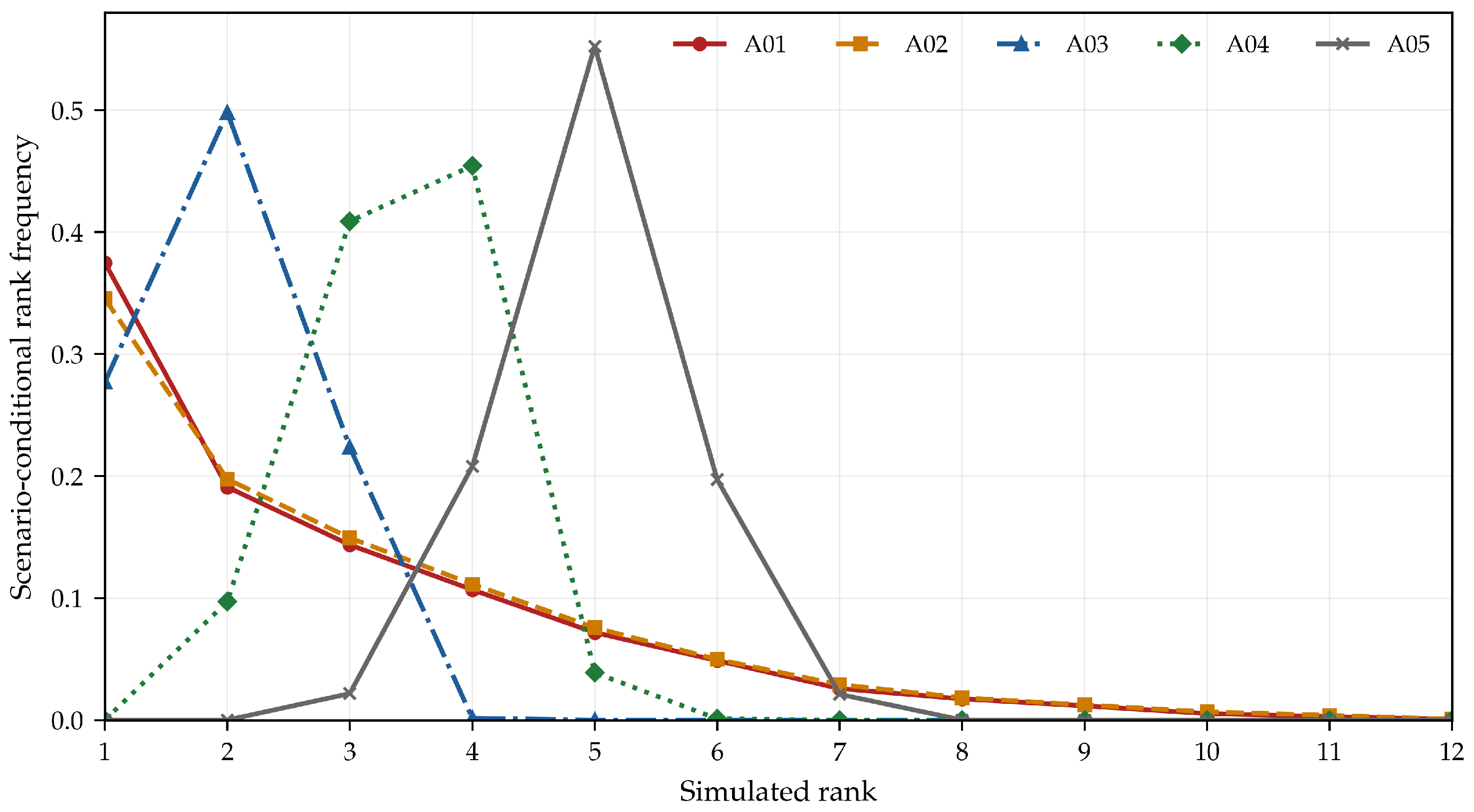
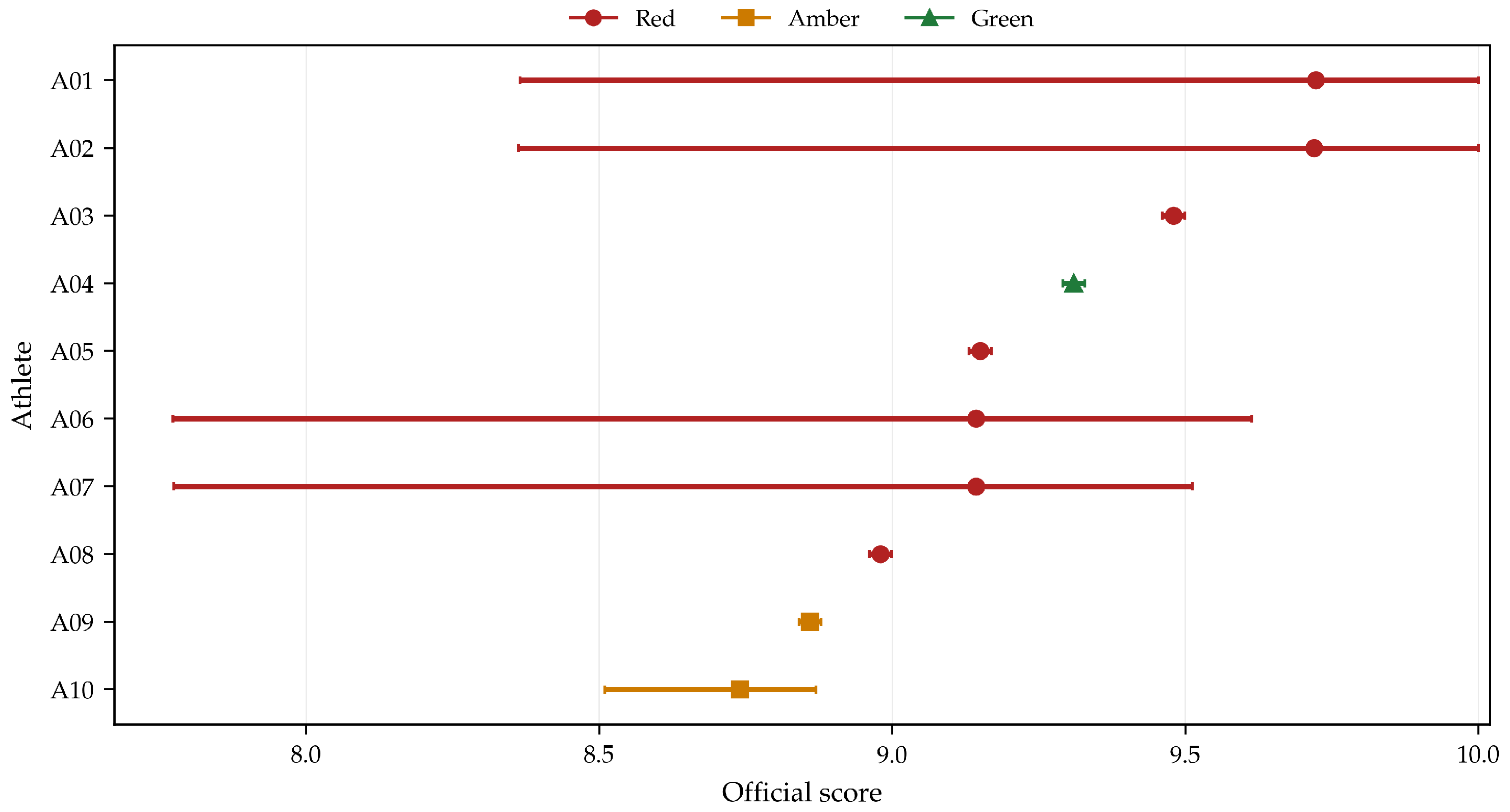
Figure 2 illustrates total screening intervals for the top ten synthetic athletes. The endpoints are exactly those in Equation (22); they combine A/C directional exposure, the deterministic B screening half-width, and directional Head Judge score effects. Marker color does not encode a Group B variation profile. Instead, it records the most severe analyst-defined synthetic adjacent-pair screening class (red/amber/green) involving that athlete and either immediate ranking neighbor in the baseline result. The figure should be read as a diagnostic display of declared perturbation states, not as a confidence interval for true performance. Figure 4 shows the corresponding Rank Cloud frequencies for selected athletes under the baseline synthetic perturbation model.

3.4. Sensitivity to Perturbation Scale and Dependence

Sensitivity to perturbation assumptions is assessed by varying the principal scenario parameters. The stress test varies A/C perturbation scale, B perturbation scale, Head Judge activation probability, and intra-athlete random effect dependence. Table 11 summarizes the aggregate scenario outputs. The scenarios do not define policy thresholds; they show how conclusions depend on the declared model.
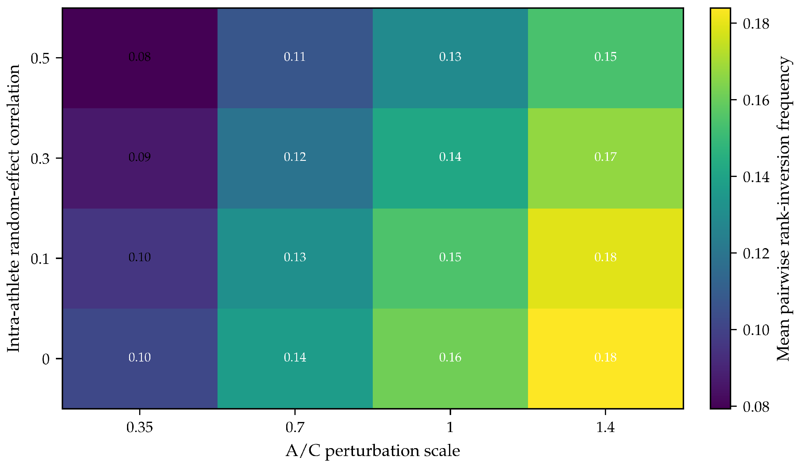
Figure 5 reports a small two-dimensional scenario grid varying the A/C perturbation scale and intra-athlete random effect correlation under the mark-level B baseline. The aggregate counts conceal one class transition in the high-perturbation scenario: one pair assigned the baseline synthetic amber class moves to the synthetic red class; all other listed scenarios preserve their baseline synthetic labels. Thus, stable counts should not be used as a substitute for pairwise transition checks, while inversion frequencies can still vary substantially. This is why empirical use should pre-specify the perturbation model or calibrate it from independent review data.

3.5. Transferability Beyond the Case Study

The method is not specific to Wushu notation. Consider a generic judged scoring rule
s i = τ w 1 y i + w 2 I { z i 1 + z i 2 1 } + w 3 trim ( b i ) h i ,
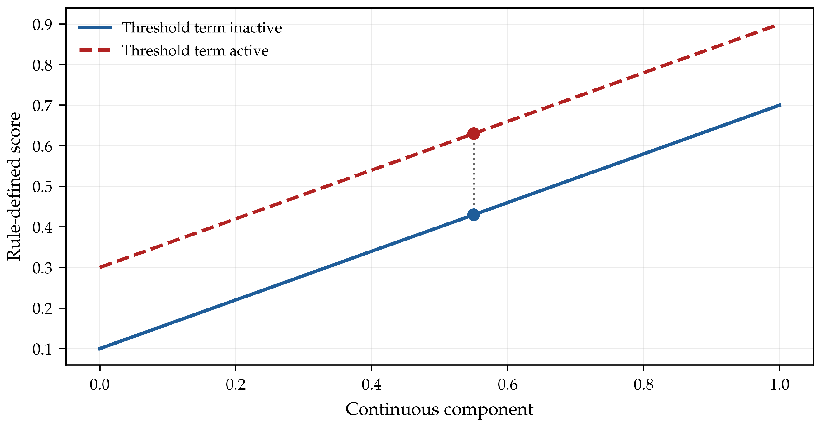
where y i is continuous, z i 1 , z i 2 are discrete decisions, trim ( b i ) is an ordered-statistic estimator, h i is an adjustment, and τ is a reporting operator. Figure 6 shows that a threshold term alone can make a small input change produce a nonlocal score jump. Any domain with a reconstructable scoring grammar and an explicit ranking rule can use the same logic.

4. Discussion

4.1. What Is New and What Is Not

The novelty lies in rule-aware reporting, not in the invention of new Monte Carlo machinery. The method combines known statistical operations in a domain where the official rule itself is nonlinear and partially discrete. The contribution is the explicit alignment of perturbation units with the official scoring grammar, the distinction between deterministic exposure and scenario-conditional Rank Clouds, and the reporting of pairwise rank sensitivity after recomputing the official ranking rule. Table 5 is therefore as important as the Monte Carlo algorithm: it prevents screening quantities from being read as probabilities.

4.2. Synthetic Demonstration Versus Empirical Validation

The stress test checks the computational behavior of the diagnostic quantities across deliberately stable, borderline, and sensitivity-active configurations. External calibration would require raw judging logs, five B marks, official tie-break variables, and independent review or repeated panels. A useful empirical endpoint would be whether pairs flagged as sensitivity-active under pre-specified rules show higher disagreement or more rank changes under independent review than pairs assigned the synthetic green class.

4.3. Bayesian Interpretation

Without empirical calibration, perturbation probabilities remain scenario inputs. A genuinely prior predictive construction is specified before conditioning on the official record; probabilities elicited after inspecting that record define a subjective predictive distribution conditional on it. A posterior predictive construction requires calibration data and an explicit likelihood. The Rank Cloud propagates whichever distribution is declared through the scoring and ranking rule; none is estimated from empirical data here.

4.4. Robustness Is Not Correctness

Rank robustness is a stability property of the official ranking rule under declared perturbations. It is not a claim that the official order equals a latent true order. A ranking may be highly robust because all perturbations preserve the order, yet still be far from a true performance order if the recorded evaluations are collectively biased. Conversely, a ranking may be sensitivity-active even when all official calls are substantively defensible. This distinction addresses the difference between rule sensitivity, rater reliability, and empirical correctness.

4.5. Applicability Beyond Wushu Taolu

The method applies to reconstructable ranking systems with four ingredients: a computable score function, observable or documentable decision units, a tie-aware ranking rule, and a declared perturbation model. Potential domains include judged sports, examination panels, grant-review panels, clinical composite scores, league tables, and other rule-based rater-mediated rankings. The substantive interpretation in each domain depends on its scoring grammar and available calibration data.

5. Limitations

The numerical study is synthetic and the perturbation model is analyst-specified; accordingly, the reported frequencies describe scenario behavior rather than empirical prevalence. Different probability scales, dependence structures, or calibration data can change Rank Cloud outputs. Empirical Wushu deployment would require raw judging logs, event-specific tie-break variables, and independent validation data. Score Cloud Analysis alone cannot identify a latent true ranking.

6. Conclusions

Score Cloud Analysis provides a rule-aware statistical method for reporting ranking robustness under discrete judgment uncertainty. It recomputes deterministic score and rank functions under finite perturbation states, separates deterministic screening diagnostics from scenario-conditional Rank Cloud frequencies, and distinguishes score ties from rank inversions. The numerical findings characterize the behavior of the method under the specified synthetic perturbation scenarios; they do not empirically confirm judging reliability, ranking correctness, or a latent true performance order. Future work should calibrate perturbation distributions using independent review or repeated panels and test whether sensitivity-active pairs show greater disagreement or rank instability than pairs assigned the synthetic green class. The method is applicable to rule-based, rater-mediated ranking systems whose scoring grammar and tie-break rule can be reconstructed.

Supplementary Materials

The following supporting information can be downloaded at: https://www.mdpi.com/article/10.3390/stats9050087/s1, Supplementary File S1: Supplementary Methods; Supplementary File S2: Reproducibility package (synthetic data, code, figures, and computational validation files).

Funding

This research received no external funding.

Institutional Review Board Statement

Not applicable. The manuscript is methodological and uses only synthetic illustrative data. Any future study using identifiable judge or athlete data should obtain the required ethical and federation approvals.

Informed Consent Statement

Not applicable.

Data Availability Statement

The synthetic data presented in this study are included in the Supplementary Materials of this article. The complete reproducibility package, including the data files (CSV and JSON), analysis scripts, and code required to reproduce the findings, is available within the Supplementary Materials. Further inquiries can be directed to the corresponding author.

Acknowledgments

The author used ChatGPT 5.6 solely for language refinement, formatting, and LaTeX support.

Conflicts of Interest

The author is affiliated with the Federazione Italiana Wushu Kung Fu e Arti Marziali Vietnamite (FIWuK). The manuscript is methodological, uses only synthetic data, and does not analyze, challenge, or reinterpret any real competition result. The manuscript uses no FIWuK competition data, evaluates no FIWuK event, and does not represent an official FIWuK decision or policy unless separately authorized.

References

  1. Goldstein, H.; Spiegelhalter, D.J. League Tables and Their Limitations: Statistical Issues in Comparisons of Institutional Performance. J. R. Stat. Soc. Ser. A Stat. Soc. 1996, 159, 385–443. [Google Scholar] [CrossRef] [Scilit]
  2. Lockwood, J.R.; Louis, T.A.; McCaffrey, D.F. Uncertainty in Rank Estimation: Implications for Value-Added Modeling Accountability Systems. J. Educ. Behav. Stat. 2002, 27, 255–270. [Google Scholar] [CrossRef] [Scilit] [PubMed]
  3. Saisana, M.; Saltelli, A.; Tarantola, S. Uncertainty and Sensitivity Analysis Techniques as Tools for the Quality Assessment of Composite Indicators. J. R. Stat. Soc. Ser. A Stat. Soc. 2005, 168, 307–323. [Google Scholar] [CrossRef] [Scilit]
  4. Saltelli, A.; Annoni, P.; Azzini, I.; Campolongo, F.; Ratto, M.; Tarantola, S. Variance Based Sensitivity Analysis of Model Output. Design and Estimator for the Total Sensitivity Index. Comput. Phys. Commun. 2010, 181, 259–270. [Google Scholar] [CrossRef] [Scilit]
  5. Borgonovo, E. A New Uncertainty Importance Measure. Reliab. Eng. Syst. Saf. 2007, 92, 771–784. [Google Scholar] [CrossRef] [Scilit]
  6. JCGM 100:2008(E); Evaluation of Measurement Data: Guide to the Expression of Uncertainty in Measurement. BIPM: Sèvres, France, 2008. [CrossRef] [Scilit]
  7. JCGM 101:2008; Evaluation of Measurement Data: Supplement 1 to the Guide to the Expression of Uncertainty in Measurement: Propagation of Distributions Using a Monte Carlo Method. BIPM: Sèvres, France, 2008. [CrossRef] [Scilit]
  8. Cohen, J. A Coefficient of Agreement for Nominal Scales. Educ. Psychol. Meas. 1960, 20, 37–46. [Google Scholar] [CrossRef] [Scilit]
  9. Fleiss, J.L. Measuring Nominal Scale Agreement among Many Raters. Psychol. Bull. 1971, 76, 378–382. [Google Scholar] [CrossRef] [Scilit]
  10. Shrout, P.E.; Fleiss, J.L. Intraclass Correlations: Uses in Assessing Rater Reliability. Psychol. Bull. 1979, 86, 420–428. [Google Scholar] [CrossRef] [PubMed]
  11. Koo, T.K.; Li, M.Y. A Guideline of Selecting and Reporting Intraclass Correlation Coefficients for Reliability Research. J. Chiropr. Med. 2016, 15, 155–163. [Google Scholar] [CrossRef] [Scilit] [PubMed]
  12. Brennan, R.L. Generalizability Theory; Springer: New York, NY, USA, 2001. [Google Scholar]
  13. Zitzewitz, E. Nationalism in Winter Sports Judging and Its Lessons for Organizational Decision Making. J. Econ. Manag. Strategy 2006, 15, 67–99. [Google Scholar] [CrossRef] [Scilit]
  14. Heiniger, S.; Mercier, H. Judging the Judges: Evaluating the Accuracy and National Bias of International Gymnastics Judges. J. Quant. Anal. Sport. 2021, 17, 289–305. [Google Scholar] [CrossRef] [Scilit]
  15. Tukey, J.W. A Survey of Sampling from Contaminated Distributions. In Contributions to Probability and Statistics; Olkin, I., Ghurye, S.G., Hoeffding, W., Madow, W.G., Mann, H.B., Eds.; Stanford University Press: Stanford, CA, USA, 1960; pp. 448–485. [Google Scholar]
  16. Huber, P.J.; Ronchetti, E.M. Robust Statistics, 2nd ed.; Wiley: Hoboken, NJ, USA, 2009. [Google Scholar] [CrossRef] [Scilit]
  17. International Wushu Federation. The International Wushu Federation (IWUF) Released the Latest Wushu Competition Rules and Judging Methods, Which Will Be Officially Implemented in 2025. 2024. Available online: https://www.iwuf.org/en/news/gjwl/2024/0914/8955.html (accessed on 30 May 2026).
  18. International Wushu Federation. Wushu Taolu Competition Rules and Judging Methods (2024); International Wushu Federation: Lausanne, Switzerland, 2024; Available online: https://www.iwuf.org/xhimg/soft/240912/WUSHU-TAOLU-COMPETITION-RULES-AND-JUDGING-METHODS-2024.pdf (accessed on 30 May 2026).
  19. Pearl, J. Causal Inference in Statistics: An Overview. Stat. Surv. 2009, 3, 96–146. [Google Scholar] [CrossRef] [Scilit]
  20. Bareinboim, E.; Correa, J.D.; Ibeling, D.; Icard, T. On Pearl’s Hierarchy and the Foundations of Causal Inference. In Probabilistic and Causal Inference: The Works of Judea Pearl; Dechter, R., Geffner, H., Halpern, J.Y., Eds.; ACM Books: New York, NY, USA, 2022; pp. 507–556. [Google Scholar] [CrossRef] [Scilit]
  21. Morris, T.P.; White, I.R.; Crowther, M.J. Using Simulation Studies to Evaluate Statistical Methods. Stat. Med. 2019, 38, 2074–2102. [Google Scholar] [CrossRef] [Scilit] [PubMed]
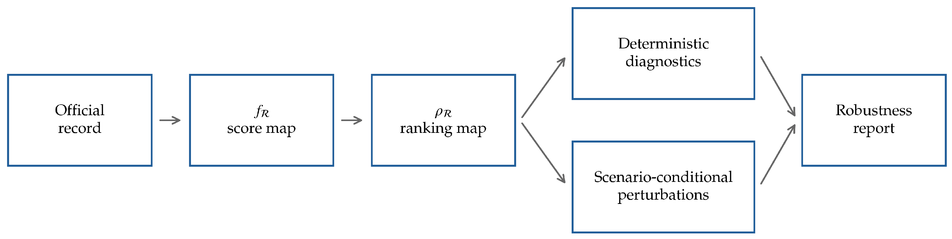
Figure 1. Rule-aware sensitivity-reporting sequence. The diagram separates official scoring, official ranking, deterministic diagnostics, scenario-conditional perturbations, and Rank Cloud outputs. Explanatory interpretation remains in the text; no empirical competition data are used.
Stats 09 00087 g001
Figure 2. Synthetic total screening intervals for the top ten athletes. Interval endpoints follow Equation (22). Marker color denotes the most severe baseline adjacent-pair screening label involving each athlete and an immediate ranking neighbor; it does not denote Overall Performance (Group B) variation. The intervals are screening envelopes, not exact Score Cloud hulls and not empirical confidence intervals.
Stats 09 00087 g002
Figure 4. Synthetic Rank Cloud for selected athletes under the baseline perturbation scenario. Point frequencies are scenario-conditional sensitivity outputs; 95% exact binomial Monte Carlo uncertainty intervals for every athlete–rank cell are supplied in Supplementary File S2. Near-overlap of some curves reflects similar scenario-conditional rank distributions rather than graphical duplication.
Stats 09 00087 g004
Figure 5. Synthetic sensitivity grid for A/C perturbation scale and intra-athlete random effect correlation. Entries are mean adjacent-pair rank inversion frequencies under the declared synthetic scenario.
Stats 09 00087 g005
Figure 6. Generic threshold component in a nonlinear scoring rule. A small change in a discrete decision state can create a jump in the rule-defined score. The solid blue line denotes the threshold-inactive branch, the dashed red line the threshold-active branch, and the vertical dotted segment marks the score jump at the illustrated input value.
Stats 09 00087 g006
Table 1. Positioning of the method relative to adjacent statistical approaches.
Related ApproachUsual TargetWhat Is Retained HereAdded Reporting Object
Uncertainty propagationDistribution of a measured or model-derived quantityMonte Carlo propagation through the complete rule-defined mapRank frequencies after official tie-break recomputation
Finite-difference sensitivityResponse to a specified input perturbationExact recomputation under thresholds, caps, trimming, truncation, and tie-break rulesDirectional score exposures and single-call rank sensitivity
Rank uncertaintyUncertainty in an ordering or league positionPairwise inversion and rank-persistence frequenciesRule-aware Rank Cloud with official tie-breaks
Rater reliabilityAgreement, severity, or variance componentsRecognition that recorded marks are rater-mediatedNo reliability, severity, or variance component is estimated without repeated empirical ratings
Robust statisticsResistance to outliers or contaminationTrimmed and winsorized summaries motivate Overall Performance (Group B) sensitivityRe-entry of discarded marks into tie-breaks can be diagnosed
Table 2. Claims and non-claims.
Supported by the MethodNot Supported Without Empirical Calibration
Sensitivity of the official scoring and ranking rule under declared perturbations.Probability that a judge, athlete, panel, or federation made an error.
Deterministic exposure and scenario-conditional Rank Cloud frequencies.True underlying athletic ranking or true performance order.
Comparison of alternative perturbation scenarios in a synthetic proof-of-concept.Prevalence of fragility in real Wushu competitions.
Identification of pairs whose ranking relation is active under the specified stress test.Operational policy thresholds or official review triggers.
Table 4. Practical workflow for perturbation model selection.
Model ChoiceUse WhenRequired InformationMain Risk
Independent callsNo evidence of shared ambiguity or panel-level dependence is available.Declared perturbation probabilities for each decision class.May understate uncertainty if calls are correlated.
Intra-athlete random effectSeveral marginal calls may share routine-level ambiguity.Repeated review or elicited intraclass dependence.Sensitivity depends on assumed dependence.
Panel-level effectRater-scale or panel interpretation may affect several marks.Repeated panels, judge logs, or calibration exercises.Confounding with athlete quality.
Bayesian predictive modelExpert beliefs or empirical data can be encoded as priors/posteriors.Prior distributions or calibration data.Results inherit prior and model assumptions.
Table 5. Principal quantities reported by Score Cloud Analysis. Definition/status distinguishes proposed diagnostics, reporting constructs, and adapted displays. CPE denotes contested-point exposure; TSE denotes total sensitivity exposure; FMR denotes fragility-to-margin ratio.
QuantityDefinition/StatusRequired InputsInterpretationNot Interpreted as
CPE i A C E i + E i + ; proposed aggregate diagnosticMarginal A/C calls and signed finite differences δ i Aggregate contested-point exposure; E i and E i + are the directional quantitiesError probability
TSE i j Equation (23); reporting construct E i , E j + , U B , i scr , U B , j scr , U H , i , and  U H , j + Ranking-active pairwise screening exposureCalibrated risk
FMRPairwise exposure divided by official margin; proposed diagnosticRelevant pairwise exposure and Δ i j ; ε regularization is used for synthetic screening and plottingExposure relative to the official marginProbability
Single-call activity L i j Δ i j , including tie-active equality; proposed diagnosticLargest ranking-relevant marginal A/C call and the tie-aware ranking ruleWhether one A/C call can activate a tie or rank changeProof of a wrong call
Score CloudImage of f R under admissible perturbation states; adapted uncertainty-set displayScoring function, admissible states, and score inputsRule-aware score support under declared statesTrue-score interval
Rank CloudDistribution of ρ R under sampled perturbations; adapted rank uncertainty displayRanking function, perturbation distribution, and tie-break variablesScenario-conditional rank frequency; finite-Monte Carlo uncertainty is reported separatelyTrue-rank probability
π ^ i j R , inv Equation (31); adapted Monte Carlo summarySimulated ranks after recomputing ρ R Scenario-conditional pairwise rank inversion frequency, reported with Equation (34)Empirical judging-error rate
Table 6. Compact mathematical properties of the principal diagnostics.
QuantityBoundednessMonotonicity/SensitivityZero Margin BehaviorModel Dependence
CPE A C Bounded by the finite sum of declared marginal A/C units and rule capsNondecreasing when same-direction marginal units are addedNot a ratio; defined independently of pairwise  marginNo
TSE Bounded by the included A/C, B screening, and directional Head Judge componentsNondecreasing in every included exposure componentDefined at zero margin; its raw ratio to margin is notNo
Raw FMRUnbounded as | Δ i j | 0 Increases with exposure and decreases with nonzero marginUndefined when Δ i j = 0 No
Epsilon-screened FMRBounded above by maximum admissible exposure divided by the chosen ε floorUsed for declared synthetic screening and plotting at zero or near-zero marginsUses max ( | Δ i j | , ε ) as a screening/display convention; the raw ratio remains undefined at zeroNo
Score CloudBounded by the image of admissible perturbation states under score capsUnder fixed f R , nested admissible sets Ω i , 1 Ω i , 2 imply nested exact Score Clouds; non-nested changes imply no monotonicityDefined at athlete levelOptional weights only
Rank CloudFrequencies sum to one over represented rank or rank/tie statesChanges with perturbation probabilities, dependence, and rule changesMay allocate mass to tie-break or residual-tie states when representedYes
Table 7. Baseline reconstruction and deterministic screening design. All values are illustrative and are not calibrated to empirical competition data.
Design ElementBaseline Value or RulePurpose
Competitors n = 30 synthetic competitorsCreates adjacent-pair relations across several official margins.
Monte Carlo replications M = 50 , 000 Gives maximum plug-in binomial Monte Carlo standard error (MCSE) near 0.0022.
A/C marginal callsBaseline outcome-reversal probability 0.28 for marginal calls; robust 3–0 calls have zero outcome-reversal probabilityControls one-vote decision perturbation activity.
Group B baseline modelFive two-decimal marks; centered Gaussian mark perturbations; mapping to the centesimal grid; clipping to the synthetic legal range [ 0.00 , 3.00 ] ; sorting, trimming, τ 3 , and  B L D recomputationPreserves the rule-aware mark-level B state and tie-break input.
Deterministic B screening widthPre-specified U B , i scr : 0.019 (low variation), 0.030 (moderate), and 0.055–0.070 (high); independent of the Monte Carlo Gaussian scaleSupplies a transparent deterministic screening width for TSE and Figure 2.
Head Judge perturbationSigned total-score changes of ± 0.10 where declared; baseline activation probability 0.12Tests directional Head Judge exposure in pairwise ranking relations.
Synthetic labelsGreen/amber/red labels defined by declared FMR, single-call, envelope-contact, zero margin, and rank frequency rulesProvides descriptive stress test classes, not operational thresholds.
Table 8. Scenario-scale and dependence specification for the synthetic stress test.
Scenario ElementDeclared ValuesPurpose
A/C scale multipliersLow 0.35, baseline 1.00, high 1.40; scaled probabilities clipped to [ 0 , 1 ] Tests sensitivity to the declared call-perturbation scale.
Group B mark scalesAthlete-level standard deviations: 0.0076 (low), 0.025 (moderate), and approximately 0.048–0.060 (high); scenario multipliers 0.50, 1.00, and 1.50Creates low-, moderate-, and high-variation mark profiles.
Group B dependenceWithin-athlete mark correlations 0.10 (low), 0.20 (moderate), and 0.65 (high)Tests dependence among marks entering the trimmed component.
Head Judge scaleActivation probabilities 0.05 (low), 0.12 (baseline), and 0.18 (high)Varies the occurrence of declared signed Head Judge states.
Intra-athlete random effectIndependent baseline; correlated scenario uses a Beta random effect with the scaled marginal-call mean and concentration α + β = 1 / ρ 1 at ρ = 0.30 Represents shared ambiguity among calls for the same athlete.
Retained-block comparisonGaussian perturbation of the retained B component, clipped to [ 0.00 , 3.00 ] ; the lower discarded mark is held at baselineProvides a compact surrogate comparison, not the baseline model.
Table 9. Selected adjacent-pair deterministic diagnostics in the baseline synthetic stress test. U B is the sum of the two athlete-level B screening half-widths and U H is the ranking-active directional Head Judge contribution.
PairMargin E i E j + U B U H TSEFMRtot,εSingle-CallLabel
A01–A020.0031.3000.3000.1160.0001.716572.00yesred
A03–A040.1700.0000.0000.0380.0000.0380.22nogreen
A06–A070.0001.3000.3000.1390.0001.7391739.00tie-break activered
A10–A110.1300.1000.0000.0490.1000.2491.92noamber
Table 10. Scenario-conditional Monte Carlo frequencies for the same selected adjacent pairs. The 95% intervals are exact binomial Monte Carlo uncertainty intervals conditional on the baseline synthetic perturbation model; they are not empirical confidence intervals for judging reliability or ranking correctness.
PairScore InversionScore TieRank InversionMCSE95% Monte Carlo Interval
A01–A020.48370.00360.48530.0022[0.4809, 0.4897]
A03–A040.00000.00000.00000.0000 [ 0 , 7.38 × 10 5 ]
A06–A070.48770.00320.48900.0022[0.4846, 0.4934]
A10–A110.03770.00680.04280.0009[0.0411, 0.0446]
Table 11. Aggregate scenario summaries. Counts are synthetic screening outputs; they are not empirical prevalence estimates.
ScenarioRedAmberGreenPairs Changing ClassMean Rank Inversion FrequencyMaximum Rank Inversion Frequency
Low perturbation1110800.0960.490
Baseline stress1110800.1620.640
High perturbation129810.1970.758
Intra-athlete random effect1110800.1410.520
Retained-block surrogate1110800.1580.625
Disclaimer/Publisher’s Note: The statements, opinions and data contained in all publications are solely those of the individual author(s) and contributor(s) and not of MDPI and/or the editor(s). MDPI and/or the editor(s) disclaim responsibility for any injury to people or property resulting from any ideas, methods, instructions or products referred to in the content.