Article

A Simulation-Based Modified Singular Spectrum Analysis Framework for Signal Extraction and the Exploration of Structured Nonlinear Temporal Behaviour


1
Department of Basic Sciences, College of Science and Health Professions, King Saud bin Abdulaziz University for Health Sciences, P.O. Box 3660, Riyadh 11481, Saudi Arabia
2
King Abdullah International Medical Research Center, King Saud bin Abdulaziz University for Health Sciences, Ministry of National Guard-Health Affairs, Riyadh 11481, Saudi Arabia
Stats 2026, 9(5), 86; https://doi.org/10.3390/stats9050086
Submission received: 26 June 2026 / Revised: 10 August 2026 / Accepted: 20 August 2026 / Published: 22 August 2026
(This article belongs to the Section Statistical Methods)

Abstract

Distinguishingstructured nonlinear temporal behaviour from stochastic variability remains a fundamental challenge in the analysis of noisy and nonstationary time series, particularly when conventional nonlinear methods are sensitive to noise and finite observational records. This study presents a simulation-based modified Singular Spectrum Analysis (SSA) framework for investigating finite-time nonlinear temporal structures through signal extraction, component-wise simulation, and eigenvalue distribution analysis. The proposed framework decomposes time series into interpretable components and systematically compares empirical behaviour with white-noise processes and canonical nonlinear benchmark systems. Using a noisy chaotic benchmark with a known three-dimensional state-space structure, a direct comparison with standard SSA criteria was conducted to examine component identification under the same benchmark setting, with the proposed framework identifying three components compared with two indicated by the conventional criteria. The methodology is demonstrated using COVID-19 case time series from the United Kingdom (UK) and the Kingdom of Saudi Arabia (KSA), together with monthly sunspot numbers as an independent application, as representative real-world time series. The modified SSA identified distinct temporal structures within these datasets, with eigenvalue distributions differing from those expected under pure white-noise processes while exhibiting similarities to canonical nonlinear benchmark systems. Reconstructed phase spaces displayed bounded attractor-like geometries consistent with structured nonlinear temporal behaviour over finite observational intervals. The proposed framework provides a complementary nonparametric statistical methodology for investigating structured nonlinear temporal behaviour in noisy observational time series through signal extraction and simulation-based benchmarking.

1. Introduction

Distinguishing structured nonlinear dynamics from stochastic variability remains a significant challenge in nonlinear time-series analysis due to overlapping statistical and dynamical properties that complicate clear differentiation [1,2,3]. Chaos theory, a mathematical framework pioneered by Edward Lorenz, investigates deterministic systems that exhibit strong sensitivity to initial conditions, where small perturbations may lead to substantially different trajectories over time [4]. Although governed by deterministic rules, such systems may display irregular and seemingly unpredictable temporal behaviour [5]. Consequently, considerable effort has been devoted to distinguishing stochastic variability from nonlinear deterministic structures in complex time series [6,7,8]. In practice, observational data from nonlinear systems are frequently influenced by measurement noise, reporting variability, and external perturbations, making strict classification purely stochastic or deterministic unrealistic. Accordingly, the focus of the present study is on identifying structured nonlinear temporal behaviour beyond stochastic variability using a data-driven SSA framework [9].
In complex observational time series, irregular temporal dynamics may arise from a combination of intrinsic nonlinear mechanisms and external influences, including measurement noise, external perturbations, behavioural changes, reporting variability, and intervention effects. Such factors complicate the distinction between structured nonlinear temporal behaviour and stochastic variability. Among real-world observational datasets, epidemiological surveillance data provide a particularly relevant example because observed case counts reflect not only disease transmission but also changes in reporting practices and public-health interventions. Throughout this study, terms such as chaotic-like behaviour and nonlinear deterministic structure refer to finite-time statistical signatures identified through data-driven analysis rather than formal proof of asymptotic deterministic chaos in the strict dynamical-systems sense. Canonical chaotic systems are therefore employed as reference benchmarks for interpreting SSA-derived patterns rather than as mechanistic models of epidemiological processes.
While the classical definition of deterministic chaos assumes noise-free conditions, real observational time series are typically affected by stochastic variability, measurement uncertainty, and external perturbations. Consequently, statistical methodologies designed to investigate structured nonlinear temporal behaviour must operate under realistic observational conditions rather than idealised deterministic settings. Nonlinear and chaotic dynamics have been studied across various natural and physical systems, with canonical benchmark systems such as the Hénon map and the Rössler system providing well-established reference models for nonlinear temporal behaviour [4,10,11]. For illustration of this, Figure 1 (left) shows a sequence generated from the Hénon map with parameters a = 1.4 and b = 0.3 , a standard benchmark in nonlinear dynamics widely adopted in previous studies [12,13] and included here as an illustrative example. Although the time series may initially appear irregular, plotting it in two-dimensional phase space (Figure 1 (right)) reveals a coherent attractor, illustrating how structured temporal behaviour can emerge from apparently irregular observations.
This illustrates a fundamental principle of nonlinear time-series analysis: temporal patterns that initially appear irregular may nevertheless reveal a coherent underlying structure when examined using appropriate statistical methodologies. COVID-19 case series, influenced by multiple interacting biological, behavioural, public-health, and reporting factors, provide representative examples of complex observational time series exhibiting substantial temporal variability. Previous studies have also explored the possibility of complex nonlinear and chaos-like behaviour in epidemic systems using mechanistic and dynamical modelling approaches [14]. Analysing such complex temporal behaviour may provide additional insight into epidemic variability and transmission dynamics. However, traditional nonlinear analysis methods, such as Lyapunov exponents, correlation dimensions, and nonlinear predictive models, may face limitations when applied to short, noisy, or nonstationary time series, making interpretation and practical implementation challenging [15,16,17,18,19,20,21]. In addition, previous studies have highlighted the challenges associated with early warning signals and nonlinear indicators in noisy COVID-19 surveillance data [22]. These challenges have motivated the development of alternative methodologies aimed at exploring structured nonlinear temporal behaviour in the presence of stochastic variability in complex time series [23,24,25]. Accordingly, the COVID-19 datasets are used in this study as representative case studies to illustrate the applicability of the proposed methodology under realistic observational conditions.
Numerous statistical and mechanistic modelling approaches have been developed for analysing complex temporal data, including ARIMA, space-time statistical models, and modified SEIQR/SEIR frameworks, with applications to COVID-19 epidemic dynamics [26,27,28].
While these approaches provide valuable insights, they often rely on parametric assumptions or focus primarily on trend estimation and forecasting. In contrast, data-driven methods such as Singular Spectrum Analysis (SSA) offer a nonparametric framework for decomposing complex and nonstationary time series into interpretable components.
Singular Spectrum Analysis (SSA) has demonstrated broad utility across diverse scientific disciplines, including genetics and biology [29], medicine [30], engineering [31], economics and finance [32], and epidemiological applications [33]. For an overview of the historical development of SSA, see [34], and for comprehensive discussions of SSA theory, applications, extensions, and modifications, see [35,36]. Previous SSA-based studies have also demonstrated its effectiveness for filtering, noise reduction, and signal extraction in real-world time series, including applications in gene expression and EEG analysis [37,38,39].
Despite these developments, distinguishing structured nonlinear temporal behaviour from stochastic variability in real-world observational time series remains a key methodological challenge, particularly when the data are influenced by measurement noise, reporting variability, behavioural changes, or external perturbations. This motivates the use of SSA as a complementary nonparametric framework for exploring structured temporal patterns in noisy observational time series without assuming a specific mechanistic model.
The primary objective of this study is methodological rather than epidemiological. Specifically, this study presents a simulation-based modified Singular Spectrum Analysis (SSA) framework that combines SSA decomposition with component-wise simulation and eigenvalue distribution analysis to investigate finite-time statistical signatures consistent with structured nonlinear temporal behaviour in noisy time series. Rather than attempting to establish formal deterministic chaos in the strict dynamical-systems sense, the proposed framework is designed to identify robust nonlinear temporal structures under realistic observational conditions while remaining applicable to noisy and nonstationary datasets. To evaluate this contribution directly, the proposed framework is further compared with standard SSA criteria on a noisy chaotic benchmark with a known three-dimensional state-space structure, allowing component identification under the two approaches to be examined within the same benchmark setting.
To demonstrate the applicability of the proposed statistical framework, COVID-19 case time series from the United Kingdom (UK) and the Kingdom of Saudi Arabia (KSA) are analysed as representative case studies exhibiting different epidemic patterns. To further illustrate the generality of the proposed framework beyond epidemiological data, monthly sunspot numbers, a series widely studied in the nonlinear dynamics literature, are additionally analysed as an independent application. These datasets are used to illustrate the methodology rather than to perform a comprehensive epidemiological comparison. By integrating SSA decomposition with simulation-based benchmarking of eigenvalue distributions, the proposed framework provides a complementary nonparametric approach for systematically comparing empirical data with stochastic and canonical nonlinear benchmark systems, thereby supporting the exploration of structured temporal patterns in complex real-world time series.
The remainder of the paper is structured as follows: Section 2 introduces the proposed methodology and algorithms. Section 3 evaluates this methodology using synthetic data, with a focus on the analysis and comparison of eigenvalue distributions for both chaotic and white-noise series, including a direct comparison between the proposed framework and standard SSA criteria. In Section 4, we describe the datasets used and present our evaluation results, including the method for determining the number of components required to effectively separate signal from noise, utilising simulation techniques on selected components to examine and compare eigenvalue distributions; the framework is applied to the COVID-19 case series and, as an additional independent application, to monthly sunspot numbers. This analysis assists in exploring structured nonlinear temporal behaviour relative to stochastic variability and in characterising chaotic-like temporal patterns. The conclusion synthesises our findings and discusses their implications for future research.

2. Materials and Methods

2.1. Mathematical Framework of Singular Spectrum Analysis

Let { y t } t = 1 N be a real-valued time series of length N. The Singular Spectrum Analysis (SSA) procedure consists of four main steps: embedding, decomposition, grouping, and reconstruction [36,40]. These steps provide a nonparametric framework for decomposing the series into interpretable components such as trend, seasonality, and noise.
Step 1: Embedding
Choose a window length L  ( 1 < L < N ) and construct the trajectory (Hankel) matrix
X = y 1 y 2 y K y 2 y 3 y K + 1 y L y L + 1 y N , K = N L + 1 .
Here, X denotes the trajectory (Hankel) matrix constructed from the original series. The columns of X represent lagged vectors of the series and capture its temporal dependence and correlation structure.
Step 2: Decomposition
Compute the singular value decomposition (SVD)
X = i = 1 L λ i U i V i ,
where λ 1 λ 2 λ L > 0 are the nonzero eigenvalues of X X , and ( U i , V i ) are the corresponding singular vectors. The eigenvalues λ i are proportional to the contribution of each component in the decomposition, quantifying how variance is distributed across the eigentriples.
Step 3: Grouping
Select a subset of r components ( 1 r L ) and form the grouped approximation
X r = i = 1 r λ i U i V i .
This separates the signal from residual noise and provides flexibility in reconstructing specific components such as trend or seasonality.
Step 4: Reconstruction
Transform X r back into a series by diagonal averaging, yielding the reconstructed signal y ˜ t . This step completes the decomposition–reconstruction cycle and produces estimates of the underlying components of the original series.
  • Objective. The proposed SSA framework is intended as a general methodology for investigating whether temporal patterns observed in noisy observational time series are more consistent with stochastic variability or with structured nonlinear temporal behaviour. For this purpose, the empirical eigenvalue distributions obtained from the data are compared with reference distributions generated from (i) white noise, representing random behaviour, and (ii) nonlinear benchmark systems such as the Hénon and Rössler maps, representing canonical examples of deterministic nonlinear dynamics. The methodology is subsequently illustrated using COVID-19 case series as representative real-world case studies and monthly sunspot numbers as an independent application. The SSA framework is theoretically well established in the literature [36,40], whereas the present study extends the conventional SSA framework by incorporating simulation-based eigenvalue distribution analysis for exploring structured nonlinear temporal behaviour.
For clarity, the nonlinear benchmark systems used for comparison are defined below.
Hénon map:
x n + 1 = 1 a x n 2 + y n , y n + 1 = b x n ,
with typical parameters a = 1.4 and b = 0.3 .
Rössler system:
x ˙ = y z , y ˙ = x + a y , z ˙ = b + z ( x c ) ,
with typical parameters a = 0.2 , b = 0.2 , and c = 5.7 .
The classical parameter values for the Hénon map ( a = 1.4 , b = 0.3 ) and the Rössler system ( a = 0.2 , b = 0.2 , c = 5.7 ) were adopted because they correspond to well-established chaotic regimes that have been extensively used as benchmark systems in nonlinear time-series analysis. These parameter settings generate stable attractors exhibiting characteristic chaotic behaviour, making them appropriate methodological reference models for evaluating the ability of the proposed framework to distinguish structured nonlinear temporal behaviour from stochastic variability.

2.2. Modified SSA Methodology

Building on the standard SSA framework described in Section 2, we now present the modified SSA methodology developed in this study. The proposed methodology extends the classical SSA procedure through simulation-based eigenvalue analysis and component-wise investigation of reconstructed signals. Its applicability is subsequently illustrated using COVID-19 case data and further demonstrated using an independent application to monthly sunspot numbers.

2.2.1. Review of the Proposed Approach

The primary objective of the proposed framework is to separate dominant temporal structures from stochastic variability in noisy observational time series by distinguishing signal components from noise. SSA first decomposes the original time series into a set of interpretable components, each representing either the dominant temporal structure (signal) or stochastic variability (noise). The proposed framework builds upon the distribution of the eigenvalues of scaled Hankel matrices introduced by Hassani et al. [41], while the statistical procedure for selecting the signal-space dimension, denoted by r, follows the methodology developed by Alharbi and Hassani [38]. Once the signal space has been identified, diagonal averaging is applied to reconstruct each signal-related component as an individual time series. Each reconstructed component is then simulated to obtain the empirical distribution of the corresponding eigenvalues of the scaled Hankel matrix. These distributions are subsequently compared with those obtained from stochastic and nonlinear benchmark systems to investigate whether the observed temporal patterns are more consistent with stochastic variability or with structured nonlinear temporal behaviour. Finally, phase-space embedding is used to visualise the reconstructed components and examine their attractor-like geometries.
Consider a Y N dimensional series of length N, where Y N = ( y 1 , , y N ) . The transformation of this series into a multidimensional series X 1 , , X K where X i = ( y i , , y i + L 1 ) T R L gives X = ( x i , j ) i , j = 1 L , K , where K = N L + 1 and L is an integer ( 2 L N / 2 ) . A matrix X is a Hankel matrix, and all the elements along the diagonal i + j = c o n s t are equal. Let B = X X T and λ i ( i = 1 , , L ), which are the eigenvalues of B taken in decreasing order of magnitude ( λ 1 λ L 0 ), and U 1 , , U L is the orthonormal system of the eigenvectors of matrix B corresponding to these eigenvalues.
The SVD of matrix X can be written as follows: X = X 1 + + X L , where X i = λ i U i V i T . The elementary matrices X i have rank 1, and U i and V i are the left and right eigenvectors of matrix X . Note that the collection ( λ i , U i , V i ) is called the i th eigentriple of the SVD. Note also that | | X | | F 2 = t r ( X X T ) = i = 1 L λ i and | | X i | | F 2 = λ i , where | | | | F denotes the Frobenius norm.
The behaviour of the eigenvalues, λ i , depends on the length of the time series, with larger series generally producing larger eigenvalues. To remove this dependence, the matrix B = X X T is divided by its trace, yielding A = B tr ( B ) , which possesses several useful statistical properties [41]. Let ζ 1 , , ζ L denote the eigenvalues of A arranged in decreasing order ( 1 ζ 1 ζ L 0 ). The empirical distributions of these eigenvalues are obtained using the proposed Monte Carlo simulation procedure based on bounded local perturbations and are subsequently used to determine an appropriate value of r for separating the signal and noise subspaces. Accordingly, the objective of the proposed framework is to characterise the statistical properties of the eigenvalue distributions in order to identify an appropriate signal-space dimension and subsequently investigate structured nonlinear temporal behaviour in noisy observational time series. The methodology is illustrated in this study using COVID-19 case series and monthly sunspot numbers.
As demonstrated in [38], the distribution of ζ 1 is positively skewed. It has been shown that the first r = c 1 eigenvalues correspond to the signal and the remainder to the noise if s k e w ( ζ c ) ( c { 1 , , L } ) is maximal, and the progression from s k e w ( ζ c ) to s k e w ( ζ L ) follows a pattern consistent with that of white noise. Similarly, the coefficients of variation and kurtosis for ζ i can be utilised in a comparable manner. Moreover, we select the first r = c 1 eigenvalues to represent the signal and the rest for noise if ρ s ( ζ c 1 , ζ c ) is minimal, and the sequence { ρ s ( ζ i , ζ i + 1 ) } i = c L 1 resembles the pattern observed for white noise [38].
The proposed statistical measures collectively provide an estimate of the signal-space dimension. The leading eigenvalues represent the dominant temporal structure, whereas the remaining eigenvalues correspond primarily to stochastic variability. To further validate this separation, the absolute Spearman correlation matrix between ζ i and ζ j is examined. Values close to zero indicate that the corresponding components are nearly orthogonal and readily separable, whereas values approaching one indicate substantial dependence between components. Since the eigenvalues associated with white noise typically exhibit high mutual correlation, this criterion provides additional support for distinguishing signal from noise [38].
Once the signal-space dimension r has been determined, each signal matrix X i ( i = 1 , , r ) is transformed into a reconstructed time series of length N using diagonal averaging. The proposed simulation procedure is then applied to each reconstructed component to estimate the corresponding eigenvalue distributions. These distributions are subsequently compared with those obtained from stochastic and nonlinear benchmark systems to investigate whether the observed temporal patterns are more consistent with stochastic variability or with structured nonlinear temporal behaviour. Finally, time-delay embedding is employed to visualise the reconstructed components and examine their attractor-like geometries.

2.2.2. Algorithmic Implementation

The algorithm consists of three stages. In the first stage, the proposed measures partition the eigenvalues into two groups, which helps determine an appropriate value of r for separability [42]. The second stage repeats Steps 1–4 of Stage 1 for each extracted component series to obtain the distribution of the new eigenvalues; a statistical assessment is then applied to distinguish between these distributions. The third stage applies time-delay embedding to visualise potential attractor-like dynamics in the reconstructed components.
Stage 1:
1.
Map the one-dimensional time series Y N = ( y 1 , , y N ) into a multidimensional series X 1 , , X K , where
X i = ( y i , , y i + L 1 ) R L ,
the window length L satisfies 2 L N / 2 , and K = N L + 1 . This step constructs the Hankel (trajectory) matrix
X = [ X 1 , , X K ] = ( x i j ) i = 1 , , L ; j = 1 , , K .
2.
Compute
A = X X tr ( X X ) .
3.
Perform the eigendecomposition A = P Γ P , where Γ = diag ( ζ 1 , , ζ L ) contains the eigenvalues of A ordered as 1 ζ 1 ζ 2 ζ L 0 , and P = ( P 1 , , P L ) is an orthogonal matrix whose columns are the corresponding eigenvectors.
4.
Use the proposed Monte Carlo simulation procedure based on bounded local perturbations to generate m perturbed copies of the original series Y N . Following the approach described in [38], each observation y i is simulated from a bounded uniform distribution with limits determined by neighbouring observations, namely [ y i a , y i + b ] , where a = | y i 1 y i | and b = | y i y i + 1 | . This procedure preserves the local temporal structure of the series while introducing controlled variability for estimating the empirical distribution of the eigenvalues. The simulation framework is intended to characterise local variability and eigenvalue behaviour under controlled perturbations, rather than to assume that epidemiological variability follows purely white-noise dynamics.
5.
Compute the coefficient of skewness for each eigenvalue distribution. If skew ( ζ c ) is maximal, and the pattern from skew ( ζ c ) to skew ( ζ L ) is similar to that of white noise, set r = c 1 .
6.
Compute the kurtosis coefficient for each eigenvalue distribution, kurt ( ζ i ) . If kurt ( ζ c ) is maximal, set r = c 1 .
7.
Compute the coefficient of variation, CV ( ζ i ) . The CV results typically divide the eigenvalues into two groups: ζ 1 , , ζ c 1 correspond to the signal, whereas the remaining eigenvalues exhibit an approximately U-shaped pattern and correspond to noise.
8.
Compute the absolute correlation matrix between the eigenvalues and visualise it using a 20-grade grayscale (white to black) corresponding to correlation values from 0 to 1. This also separates the eigenvalues into two groups: ζ 1 , , ζ r corresponding to the signal, and the remaining eigenvalues corresponding to noise.
Stage 2:
1.
For i = 1 , , r , construct the ith elementary matrix
S ˜ i = X i = λ i U i V i ,
where λ i is the ith eigenvalue of X X , and U i and V i are the corresponding left and right singular vectors.
2.
Obtain the reconstructed one-dimensional component S ˜ i by diagonal averaging of S ˜ i (the approximation associated with X i ), for i = 1 , , r .
3.
Repeat Steps 1–4 of Stage 1 to obtain the distribution of the new eigenvalues for each reconstructed component S ˜ i ( i = 1 , , r ).
4.
Apply a statistical test for comparison between the resulting eigenvalue distributions.
Stage 3: Apply time-delay embedding to the extracted components, using varying delay values, to reveal structured and bounded trajectories and potential attractor-like behaviour.
Results are assessed component-wise using the above criteria (distributional shape, CV, skewness, kurtosis, eigenvalue correlations, and phase-space structure).

2.2.3. Extension of the Proposed SSA Framework

The proposed methodology extends both classical SSA and our previous simulation-based SSA framework. Classical SSA decomposes the original time series into interpretable components through embedding, singular value decomposition, grouping, and reconstruction, with the dominant eigentriples typically identified from the eigenspectrum obtained from a single trajectory matrix. In our previous work [38], this framework was extended by introducing repeated simulations to estimate the empirical distributions of the normalised eigenvalues, ζ i , together with their associated statistical properties, including skewness, kurtosis, coefficients of variation, and correlations, thereby providing additional statistical criteria for signal–noise separation. The present study extends this methodology further. After identifying the dominant signal components using simulation-based eigenvalue analysis, each reconstructed SSA component is treated as an individual time series and analysed separately using the same simulation framework. This component-wise analysis enables the empirical eigenvalue distributions of the reconstructed components to be compared systematically with stochastic and canonical nonlinear benchmark systems. Furthermore, time-delay embedding is applied to the reconstructed components to investigate whether they exhibit bounded attractor-like temporal patterns. Consequently, the proposed framework extends the previous methodology beyond signal extraction and signal–noise separation towards the investigation of structured nonlinear temporal behaviour in noisy observational time series. For clarity, the principal methodological differences between standard SSA and the proposed modified SSA framework are summarised in Table 1. The proposed framework extends the conventional SSA procedure by incorporating simulation-based analysis of reconstructed components, statistical characterisation of empirical eigenvalue distributions, and comparison with stochastic and canonical nonlinear benchmark systems. This comparison is examined using a noisy chaotic benchmark system in Section 3.

3. Synthetic Data Analysis

The synthetic data experiments presented in this section are intended to evaluate the behaviour of the proposed SSA framework under controlled noisy conditions. In these experiments, additive white noise is introduced intentionally to benchmark the behaviour of the eigenvalue distributions and assess separability properties under controlled noisy conditions. This controlled validation setting should be distinguished from analyses of real observational time series, where temporal variability may arise from multiple sources, including measurement uncertainty, reporting variability, behavioural changes, and external interventions. COVID-19 case series are subsequently used as representative real-world case studies, with monthly sunspot numbers included as an additional independent application.
Previous work by Alharbi and Hassani [38] demonstrated that the proposed SSA framework could be applied successfully to diverse synthetic datasets, including canonical nonlinear benchmark systems under varying signal-to-noise ratio (SNR) conditions. These studies showed that the framework remains effective across both low- and high-noise settings. The following experiments further illustrate the robustness of the proposed methodology using the Hénon and Rössler benchmark systems.

3.1. Selection of the Required Number of Eigenvalues, r

The time series generated by the chaotic Rössler system was analysed using the proposed framework to illustrate its effectiveness in determining the appropriate value of r. The Rössler system, governed by a set of differential equations, provides a canonical benchmark for nonlinear temporal behaviour. A simulated Rössler time series with additive white noise was used as the benchmark dataset for evaluating the proposed framework. The primary objective of this analysis is to demonstrate how the proposed framework identifies the number of significant eigenvalues required for effective signal–noise separation in noisy observational time series. The resulting methodology is subsequently applied to the COVID-19 case studies presented in Section 4.
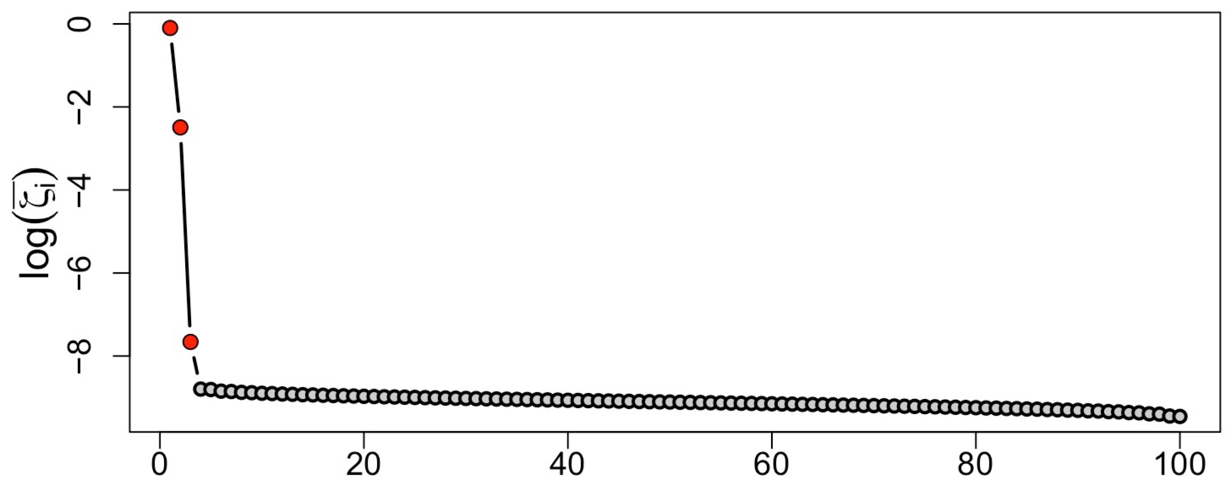
To implement the proposed approach, a large number of independent white-noise realisations were generated and added to the known Rössler signal. This controlled procedure is distinct from the bounded local perturbation scheme used for observational data, where the underlying noise-free signal is unknown. The resulting independent time series Y N m were then analysed using a window length L = 100 . The value of m was chosen to ensure a sufficiently large number of simulations for robust analysis, specifically m = 10 , 000 , as the empirical eigenvalue distributions converged and remained stable across repeated simulations. For these time series, we examined the behaviour of the eigenvalues ζ i ( i = 1 , , L ) of matrix A and their associated statistical properties. The logarithm of the mean eigenvalues is depicted in Figure 2.
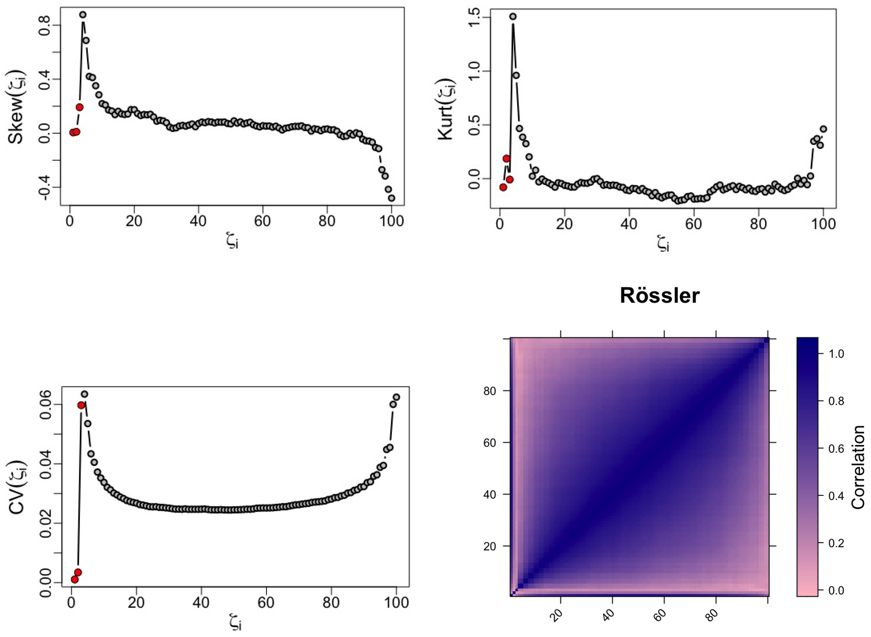
The first three eigenvalues exhibit substantially larger magnitudes than the remaining eigenvalues, indicating that the dominant temporal structure is concentrated within the first three components. Each eigenvalue contributes to the decomposition of the trajectory matrix, and the ratio 100 ζ ¯ i serves as a characteristic descriptor of matrix H i , as defined earlier. Consequently, 100 × i = 1 r ζ ¯ i characterises the optimal rank-r approximation of matrix H . The cumulative contribution of the first three eigentriples is approximately 99%, indicating that these components capture the dominant temporal structure of the signal. Figure 3 displays several measures: S k e w ( ζ i ) (top left), K u r t ( ζ i ) (top right), C V ( ζ i ) (bottom left), and the matrix of the absolute correlations between the eigenvalues (bottom right). The skewness coefficient separates the eigenvalues into two distinct groups. Notably, ζ c = 4 exhibits the highest skewness value, and the skewness pattern from ζ 4 to ζ L mirrors the behaviour associated with the noise component, as discussed in [38]. Consequently, the signal is primarily associated with the first three eigenvalues, whereas the remaining eigenvalues correspond predominantly to stochastic variability.
The kurtosis and coefficient of variation (CV) measures yield similar results, further confirming that the second group of eigenvalues corresponds to the noise component, consistent with the findings in [38,39,41]. Additionally, the correlation matrix provides further evidence, demonstrating that the Rössler signal is predominantly described by the first three leading eigenvalues, while the large square in the matrix represents the noise component. This clear separation between the two regions is consistent with the separability principle underlying SSA, indicating that the dominant signal components can be distinguished from stochastic variability.
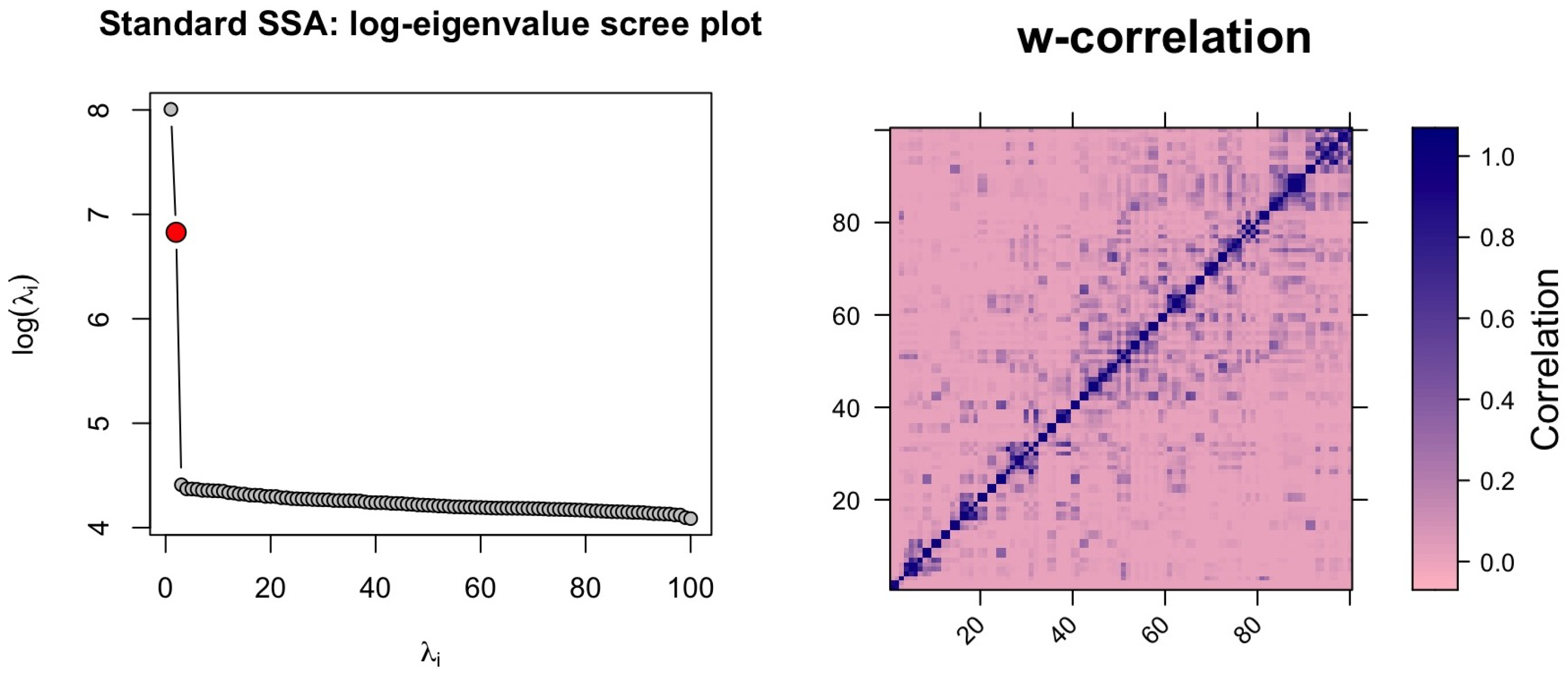
For comparison, two standard SSA criteria were applied to the same noisy Rössler realisation: the classical log-eigenvalue scree plot and the conventional w-correlation grouping criterion [36]. It should be emphasised that the repeated simulation of the noisy series is an integral component of the proposed framework, whereas conventional SSA criteria are applied directly to the observed noisy realisation; thus, each approach is implemented according to its intended methodological procedure. Both criteria identified r = 2 , corresponding to the dominant oscillatory pair of components (Figure 4, left and right, respectively), whereas the proposed simulation-based diagnostics presented above (Figure 3) identified r = 3 . In this benchmark setting, the proposed framework therefore retained the three-component structure represented in the simulated system, while the conventional SSA criteria emphasised the dominant two-component structure. This comparison illustrates that the approaches may provide complementary information because they characterise component structure using different methodological criteria. Table 2 summarises this comparison.

3.2. Comparison of Eigenvalue Distributions for Chaotic and White-Noise Series

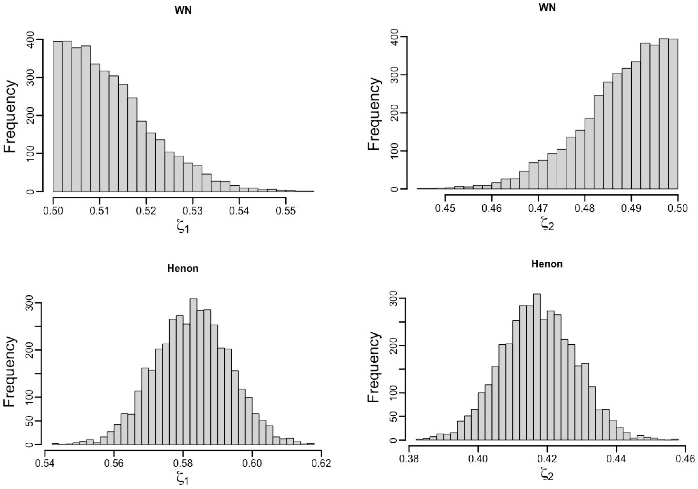
The distribution of eigenvalues ζ i was then examined by simulating two series of length N from a Hénon system and a normal distribution, repeated m times. A fixed window length of L = 2 was employed for consistency and to allow for direct comparison in subsequent sections. The initial values for the Hénon series were randomly sampled from a uniform distribution using the classical Hénon map parameters of a = 1.4 and b = 0.3 . We performed 10 3 simulations of ζ i ( i = 1 , 2 ) for both Hénon and white-noise series, examining the empirical distribution of ζ i for both. For visualisation, we set L = 2 for the embedding dimension, consistent with the two-dimensional structure of the Hénon map. Although the white-noise and Hénon series exhibit markedly different underlying dynamics, these differences are not readily apparent from the observed time series alone, particularly under noisy conditions. However, clear distinctions emerge when the empirical distributions of ζ i are examined. As shown in Figure 5, the white-noise series exhibits skewed distributions for ζ 1 and ζ 2 , whereas the Hénon series displays approximately symmetric distributions. The skewness coefficients ζ i ( i = 1 , 2 ) for both cases are summarised in Table 3, where the white-noise process shows significant skewness, unlike the Hénon series. Additionally, the D’Agostino–Pearson normality test [43] (Table 4) indicates that the Hénon series is consistent with a symmetric distribution, whereas the white-noise series is not. The significance of the observed skewness was further assessed using both the D’Agostino–Pearson and Kolmogorov–Smirnov normality tests across multiple simulations.
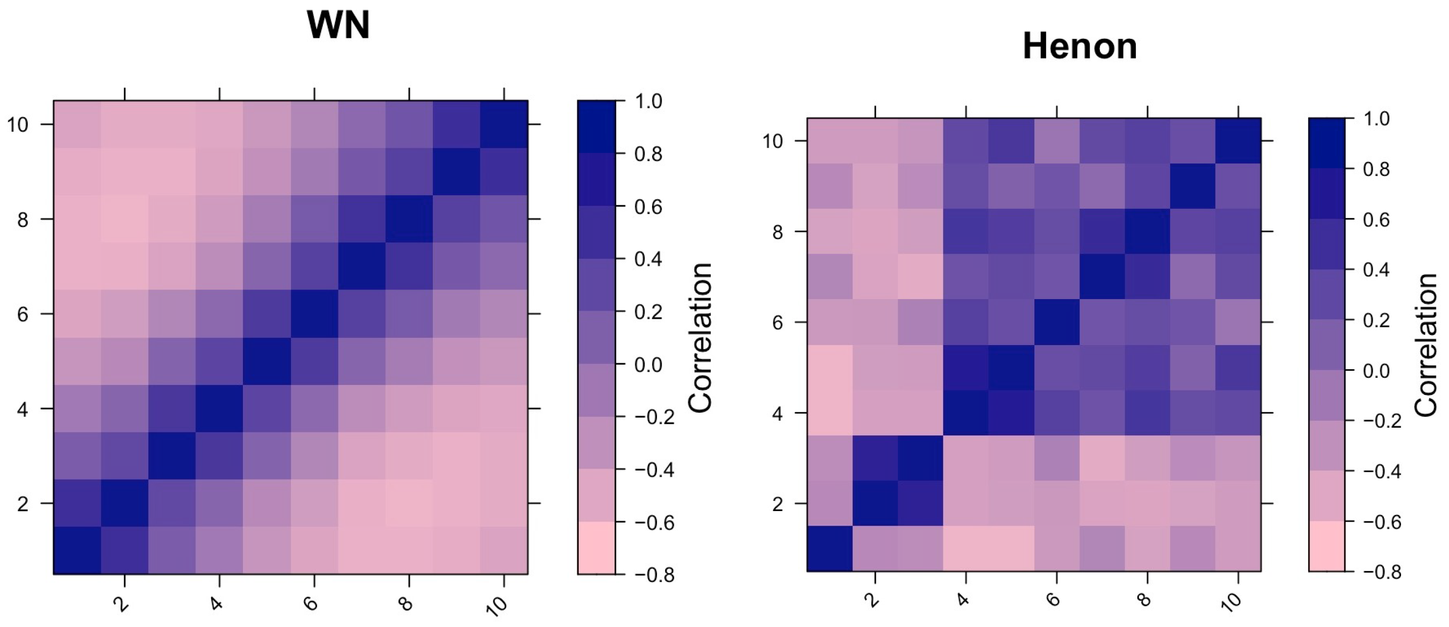
The Spearman correlation matrix for ζ i with L = 10 (Figure 6) reveals distinct correlation structures for the Hénon and white-noise series. The white-noise series exhibits stronger correlations among neighbouring eigenvalues, whereas the Hénon series displays a markedly different correlation pattern. Together, the D’Agostino–Pearson and Kolmogorov–Smirnov tests support the simulation-based comparisons, demonstrating statistically significant differences between the empirical eigenvalue distributions of the Hénon and white-noise series. In all cases, the Kolmogorov–Smirnov test rejected the null hypothesis that both series share the same distribution ( p < 0.01 ), supporting the robustness of the proposed simulation-based framework under controlled conditions.
Based on these synthetic data experiments, the proposed framework was used to compare empirical eigenvalue distribution behaviour with reference stochastic and nonlinear benchmark systems. When the observed distributions more closely resembled canonical nonlinear benchmark systems (e.g., Hénon or Tent maps), the corresponding temporal patterns were interpreted as being consistent with structured nonlinear temporal behaviour. In contrast, distributions resembling white-noise behaviour were interpreted as being more consistent with stochastic variability. This framework provides an exploratory nonparametric approach for characterising complex temporal structure in real-world observational time series and is subsequently illustrated using COVID-19 case data and monthly sunspot numbers.

4. Results

The proposed modified SSA framework was applied to representative COVID-19 case series from the UK and KSA, and, as an independent application, to monthly sunspot numbers, to illustrate its applicability for exploring structured nonlinear temporal behaviour under noisy observational conditions. The analysis combined SSA decomposition, eigenvalue distribution analysis, simulation-based benchmarking, and phase-space reconstruction to investigate finite-time temporal patterns potentially consistent with nonlinear dynamics. Multiple statistical indicators are evaluated across both UK and KSA datasets, and the results are presented through graphical visualisations illustrating the temporal structure of the reconstructed components.
For clarity, in this study the observed patterns are interpreted as finite-time statistical signatures consistent with structured nonlinear temporal behaviour rather than formal dynamical proof of deterministic chaos. Within the modified SSA framework, a component was interpreted as exhibiting structured nonlinear temporal behaviour when: (i) its empirical eigenvalue distributions ζ i resembled those generated by canonical nonlinear benchmark systems (e.g., Hénon, Rössler, Tent) and differed from white-noise surrogates; (ii) skewness, kurtosis, coefficient of variation, and Spearman correlations between successive eigenvalues indicated separation between signal and noise; (iii) the ζ -correlation matrix displayed clear block-structured grouping; and (iv) phase-space reconstructions produced bounded and organised attractor-like structures. These convergent indicators constitute the modified SSA criteria used to explore structured nonlinear temporal behaviour relative to stochastic variability in the COVID-19 time series.

4.1. Analysis of COVID-19 Data

The UK and KSA were selected as representative case studies because they exhibit distinct epidemic trajectories, reporting characteristics, and public-health responses. These differences provide an opportunity to illustrate the applicability of the proposed framework across contrasting real-world observational datasets.
To apply the proposed framework to real-world observational data, multiple simulated realisations were generated from the original COVID-19 case series using the bounded local perturbation procedure described in Section 2.2. This simulation-based strategy enabled the empirical investigation of eigenvalue distributions, which formed the basis for distinguishing structured nonlinear temporal behaviour from stochastic variability.
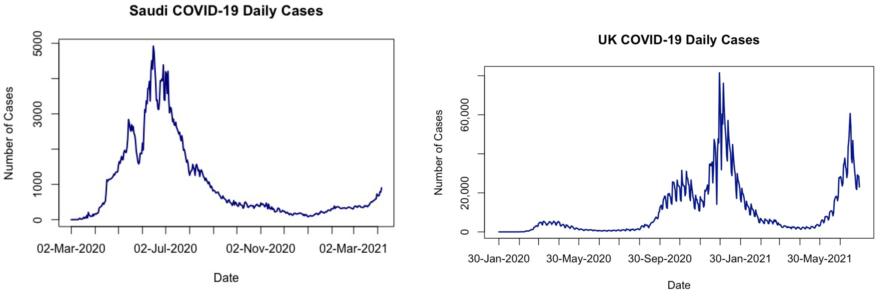
This study applies the proposed framework to two real-world COVID-19 case series: confirmed daily cases in the KSA from 2 March 2020 to 7 April 2021 (Figure 7), obtained from official national health authority reports as archived and publicly accessible via the World Health Organization (WHO) COVID-19 Dashboard (accessed on 7 August 2021) [44], and confirmed daily cases in the UK from 30 January 2020 to 29 July 2021, obtained from the UK Government Coronavirus Dashboard (accessed on 7 August 2021) [45]. The UK dataset covers a longer observation period than the KSA dataset. This difference does not affect the analysis because SSA can be applied to time series of different lengths, including relatively short observational series.
The analysis of these datasets, representing different epidemiological and socio-political contexts, provides an opportunity to examine structured nonlinear temporal patterns across contrasting noisy epidemiological observations. Importantly, the observed differences between the UK and KSA are not assumed a priori but are derived from the SSA decomposition and supported by statistical comparisons of the reconstructed components. To provide context, Table 5 reports the key descriptive statistics of the original COVID-19 daily case series for the UK and KSA. The daily confirmed case series were analysed as reported by the original data sources. No smoothing, transformation, normalisation, or adjustment for weekly reporting cycles was applied prior to the SSA. The datasets contained no missing daily observations, and days with zero reported cases were retained without modification.
Table 5 shows that both datasets are positively skewed, reflecting the presence of extreme daily case values, which is typical of epidemic data. The UK series also exhibits high kurtosis, while the KSA series has lower kurtosis but remains positively skewed. These characteristics further justify the use of SSA, as it is robust to non-normality and capable of extracting meaningful structure from noisy, skewed time series. The reconstructed SSA components analysed in subsequent sections are interpreted as dominant temporal structures extracted from noisy epidemiological observations rather than exact mechanistic representations of epidemic transmission dynamics.

4.1.1. Selection of the Number of Eigenvalues r

The selection of the window length L depended on the characteristics and objectives of each analysis. For the COVID-19 case series, values such as L = 7 were considered to account for short-term temporal structure and weekly reporting patterns commonly observed in epidemiological surveillance data. Larger values of L were additionally explored to assess the stability and robustness of the SSA decomposition under different embedding conditions and to capture broader temporal variability in the reconstructed dynamics. For the synthetic benchmark systems, smaller embedding dimensions were also examined where appropriate, consistent with the underlying dimensional structure of the simulated systems.
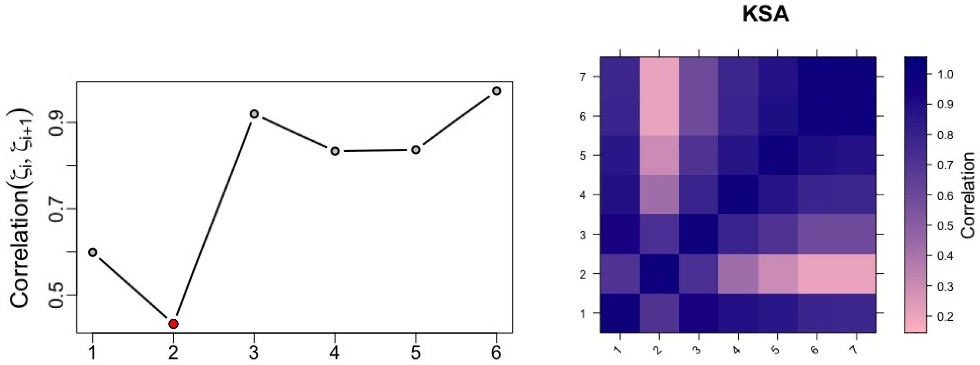
To further elaborate on the selection of r for our study, we have utilised daily confirmed COVID-19 case data, aligning with findings from a previous study that determined that a window length L = 7 yields the most accurate results with an optimal r of value 2 [42]. In this context, and for consistency with that earlier setup, part of our analysis also considered the first 42 values from the Saudi dataset when applying L = 7 . However, in the present work, the full dataset was primarily analysed using larger window lengths to capture more comprehensive dynamics. This precision in choosing r stems from an intricate analysis of matrix correlations, specifically the correlation between consecutive eigenvalues ζ i and ζ i + 1 , within the chosen window length, as detailed in prior work [42]. The Spearman correlation matrix analysis, comparing ζ i and ζ j across all values from 1 to 7, effectively segregated the eigenvalues into two principal groups. The pivotal observation leading to the selection of r = 2 was the minimal Spearman’s ρ s value between ζ c 1 = 2 and ζ c = 3 , as illustrated in this study’s findings (see Figure 8). This analytical method not only underscores the robustness of the proposed selection criterion for r, but also enhances the reliability of the subsequent signal–noise separation and nonlinear temporal analysis. The resulting framework provides a systematic methodology for investigating structured nonlinear temporal behaviour in noisy observational time series and is illustrated in the present study using COVID-19 case data.

4.1.2. Comparison of Eigenvalue ζ i Distributions

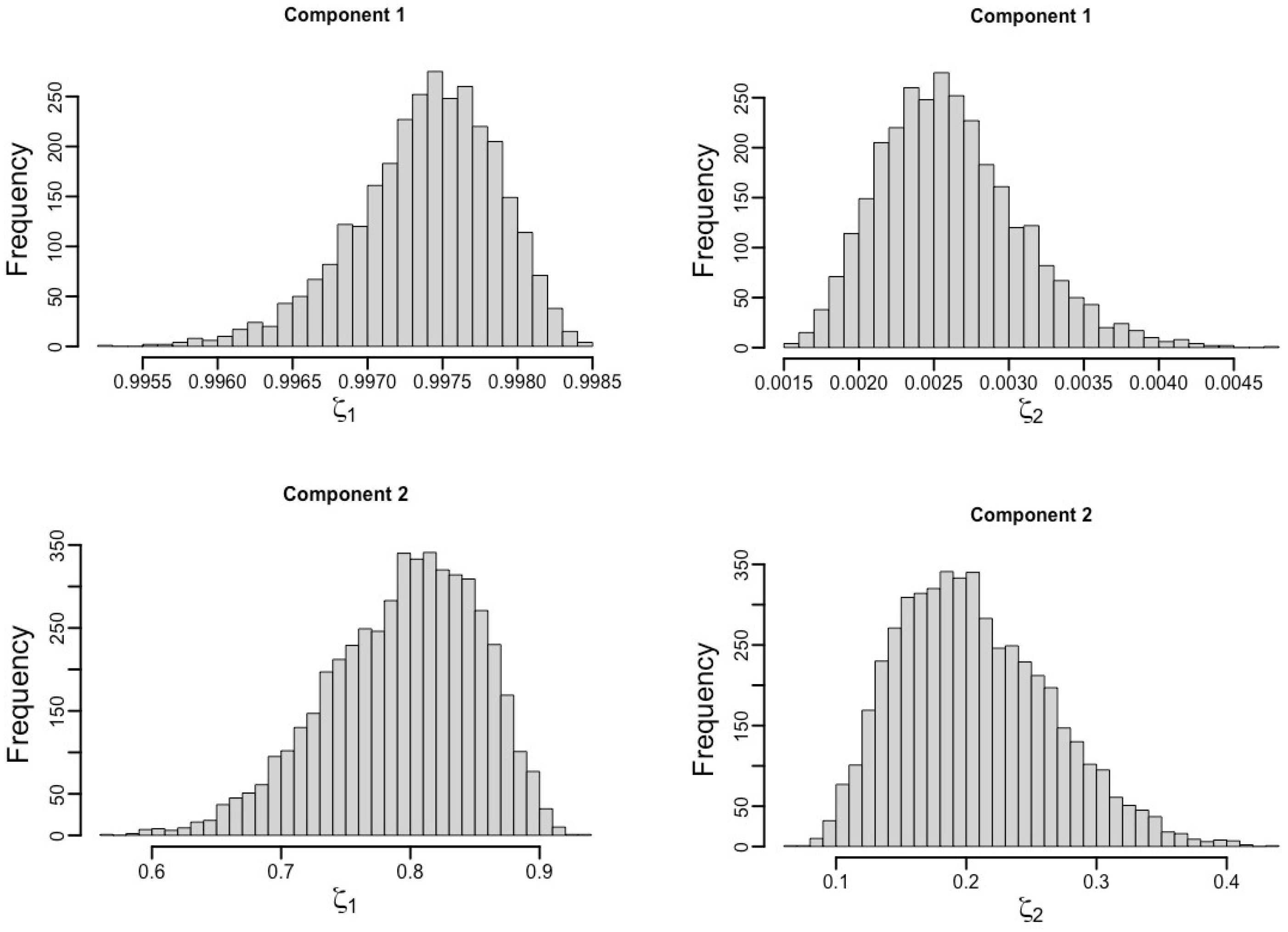
This subsection delves into a comprehensive analysis of eigenvalue distributions from COVID-19 data across the KSA and UK, incorporating a range of window lengths to explore the dynamics deeply. For a granular window length of L = 2 , this study meticulously simulates each component, uncovering a distinct eigenvalue distribution ( ζ i ) for the KSA data that deviates significantly from the patterns typical of white-noise processes (see Figure 9). This deviation is particularly pronounced in the first component Figure 9 (top), aligning closely with distributions observed in chaotic tent series, suggesting temporal patterns consistent with structured nonlinear behaviour relative to stochastic benchmark processes (for more information refer to [37]).
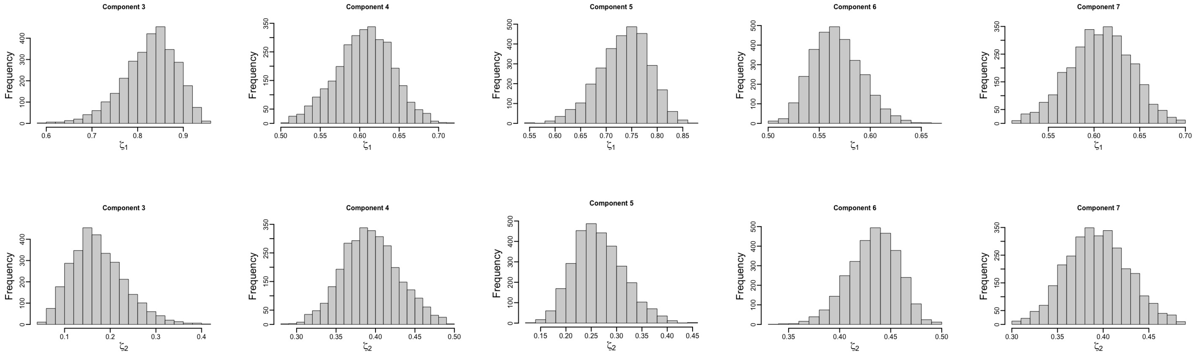
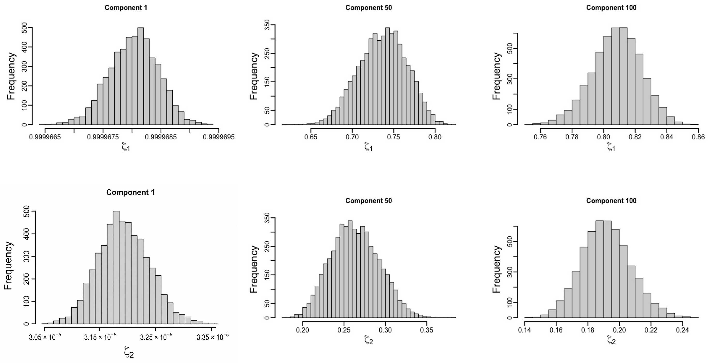
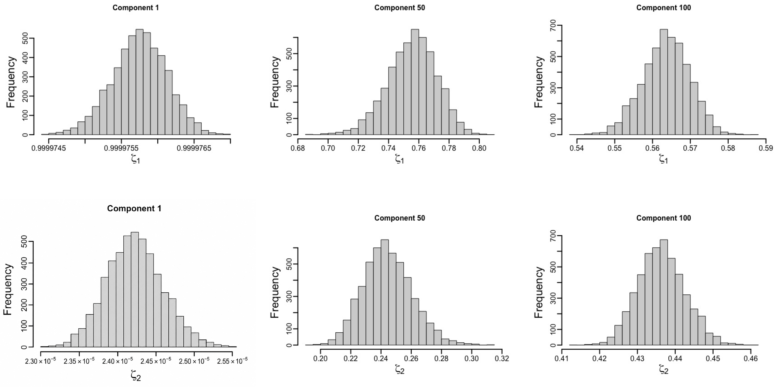
Expanding the analysis to L = 7 , as previously established by Alharbi [42], a similar divergence in the distributions of ζ i = 1 , 2 was observed for the third to seventh reconstructed components (Figure 10). In particular, the third component exhibited characteristics similar to those observed in nonlinear benchmark systems, suggesting temporal behaviour consistent with structured nonlinear dynamics in the COVID-19 time series. This pattern was consistently observed across both the KSA and UK datasets. Further extending the analysis to L = 100 , the largest, middle, and smallest reconstructed components were compared with canonical nonlinear benchmark systems and white-noise processes. Across both datasets, the empirical eigenvalue distributions exhibited greater similarity to the nonlinear benchmark systems than to white-noise behaviour (Figure 11 and Figure 12).
These analyses suggest the presence of structured nonlinear temporal patterns within the COVID-19 datasets and demonstrate the utility of eigenvalue distribution analysis for distinguishing structured dynamics from stochastic variability. The results highlight the potential of the proposed SSA-based framework for exploring complex temporal behaviour in epidemiological data while emphasising that the observed patterns should be interpreted cautiously within the limitations of noisy real-world surveillance data.
Across both the UK and KSA datasets, the empirical eigenvalue distributions differed substantially from those observed for white-noise processes, while exhibiting qualitative similarities to the canonical nonlinear benchmark systems considered in this study (Hénon and Rössler). These comparisons support the interpretation that the observed temporal patterns are more consistent with structured nonlinear temporal behaviour than with purely stochastic variability, while recognising that the benchmark systems serve only as methodological references rather than as mechanistic epidemiological models.

4.1.3. Attractor-like Patterns

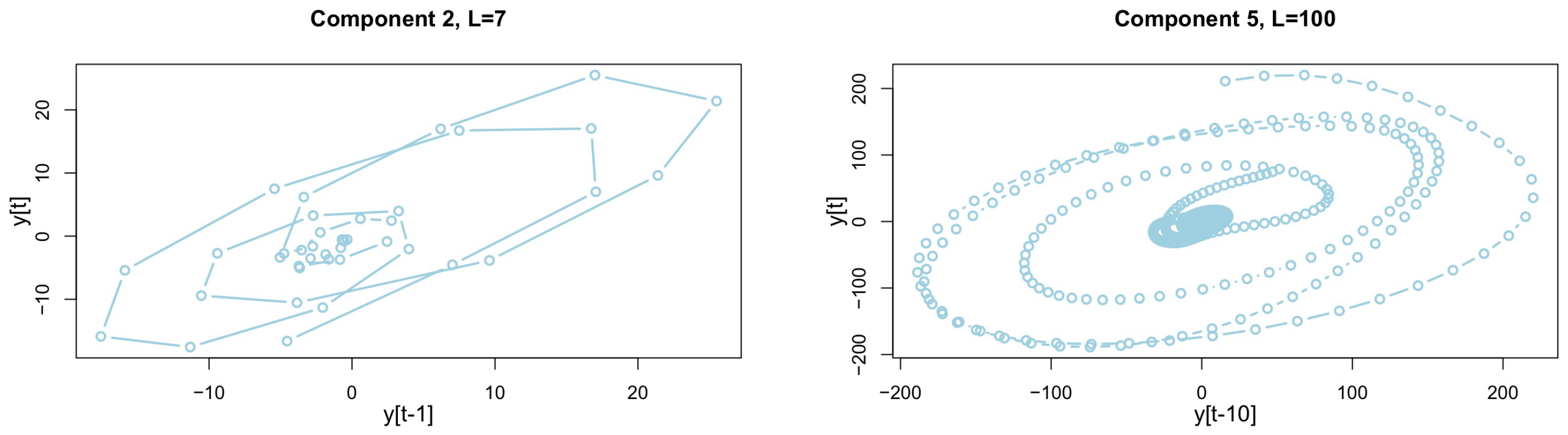
The proposed framework was further used to investigate attractor-like (chaotic-like) patterns in the COVID-19 case series from the UK and KSA by means of component-wise analysis using the proposed statistical criteria (skewness, kurtosis, coefficient of variation, and eigenvalue correlation structure), followed by time-delay embedding to examine phase-space structure. For the KSA, analysis with L = 7 revealed a structured and bounded pattern in the second component, consistent with structured nonlinear temporal behaviour rather than purely stochastic variability. With L = 100 , the fifth component exhibited a stable, oscillatory, bounded trajectory in phase space, indicating attractor-like behaviour in the underlying process (see Figure 13).
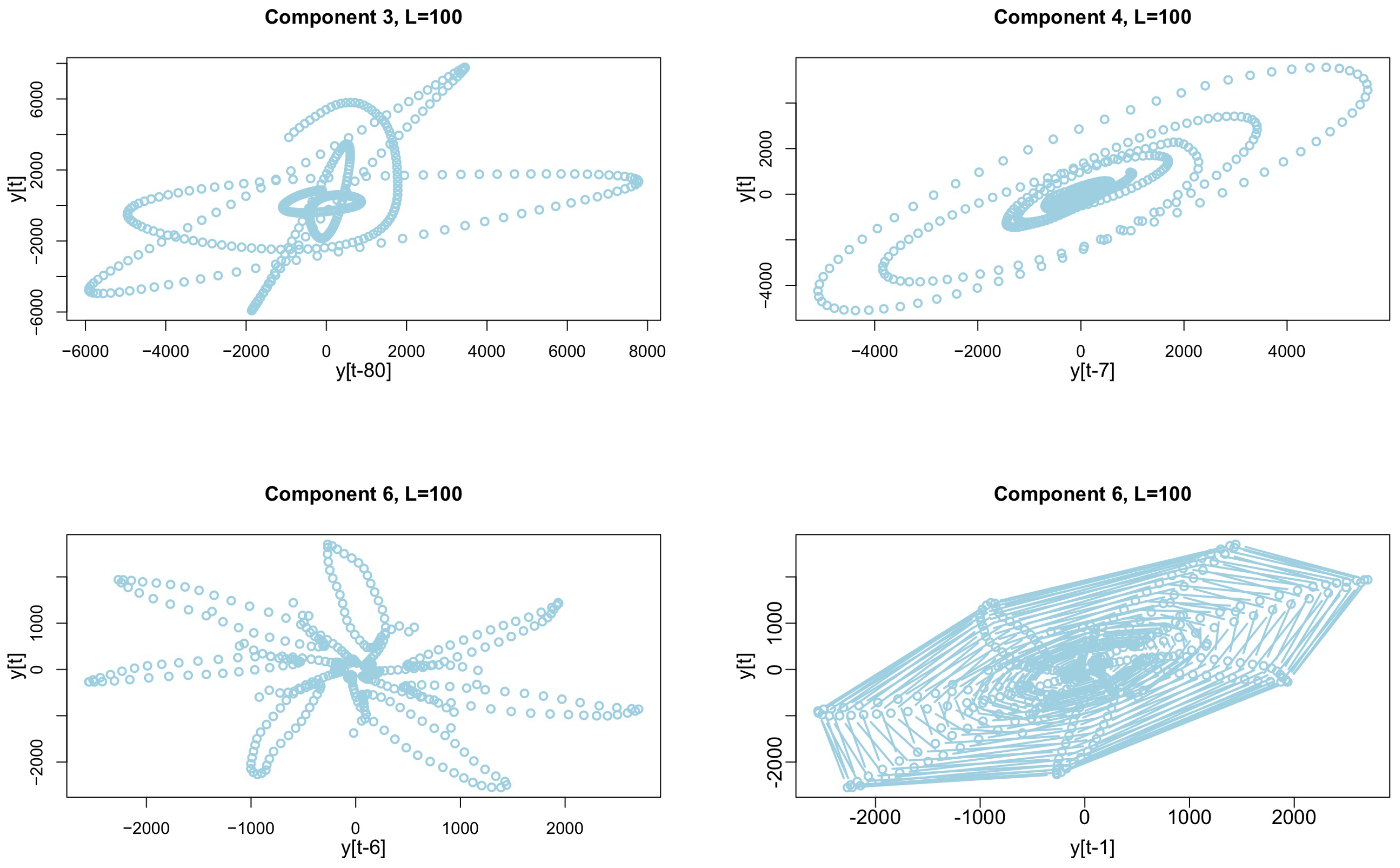
For the UK case series, a broader spectrum of unusual patterns was observed, particularly at L = 100 , across the third, fourth, and sixth components, each with its distinct time delays; the results are depicted in Figure 14. The sixth component, for instance, displayed a complex bounded structure that could be likened to a floral arrangement with seven leaves (Figure 14 (bottom left)) or a spider’s web (Figure 14 (bottom right)), showcasing the data’s intricate and potentially chaotic nature. The transition from predominantly stochastic variability toward more structured nonlinear temporal behaviour in the UK dataset was observed in the third component of the reconstructed phase space when the embedding dimension was L = 100 . For the KSA dataset, this transition occurred in the fifth component under similar conditions. These findings were corroborated by the eigenvalue distributions, which showed a distinct shift from stochastic variability toward structured nonlinear temporal behaviour, as visualised in Figure 13 and Figure 14.
These patterns, particularly evident in specific components and time delays, highlight the temporal complexity present within the COVID-19 datasets. From an epidemiological perspective, the identification of structured temporal behaviour may provide complementary information for characterising changes in epidemic variability and temporal instability. However, the reconstructed patterns should not be interpreted as direct indicators of transmission mechanisms, intervention effects, or future epidemic changes. Further methodological and epidemiological validation would be required before such patterns could be considered for forecasting or public-health monitoring applications.
Although the primary objective of the present study is methodological rather than epidemiological, the differing temporal structures identified in the UK and KSA case series may reflect differences in epidemic evolution, public-health interventions, reporting practices, and population behaviour. These findings illustrate the ability of the proposed modified SSA framework to distinguish different temporal characteristics in real-world observational time series. They should not, however, be interpreted as evidence of specific epidemiological mechanisms or causal relationships.
Application of the proposed modified SSA framework to representative COVID-19 case series from the UK and KSA demonstrated its applicability for identifying structured nonlinear temporal patterns consistent with chaotic-like behaviour under noisy observational conditions. The reconstructed components together with the eigenvalue distribution analysis demonstrated the ability of the proposed framework to characterise complex temporal structures within the observed series. These findings suggest the presence of structured nonlinear temporal behaviour consistent with chaotic-like dynamics while recognising the challenges associated with interpreting complex real-world epidemiological time series influenced by multiple external factors. Several recent studies have explored SSA and related nonlinear approaches in epidemiological and complex time-series analysis [33,42]. However, the present work differs by integrating SSA with simulation-based eigenvalue distribution analysis and component-wise assessment of reconstructed dynamics. In this framework, the number of eigenvalues r is selected using statistical diagnostics, including skewness, kurtosis, coefficients of variation, and eigenvalue-correlation structure, together with comparisons against stochastic and nonlinear benchmark systems. To further assess the generality of the proposed framework beyond epidemiological surveillance data, the following subsection applies the same methodology to an independent observational series.

4.2. Monthly Sunspot Numbers

In this section, we further demonstrate the applicability of the proposed framework by considering another application: monthly sunspot numbers, a series widely reported in the literature to exhibit chaotic behaviour. Several independent analyses have reported evidence consistent with low-dimensional chaotic dynamics in sunspot records [46,47], while other work has cautioned that stochastic variability superposed on a simple periodic skeleton can produce similar signatures, and that no fully conclusive evidence for deterministic chaos in solar activity currently exists [48]. This unresolved question makes sunspot activity a well-motivated and independent test case for the proposed framework.
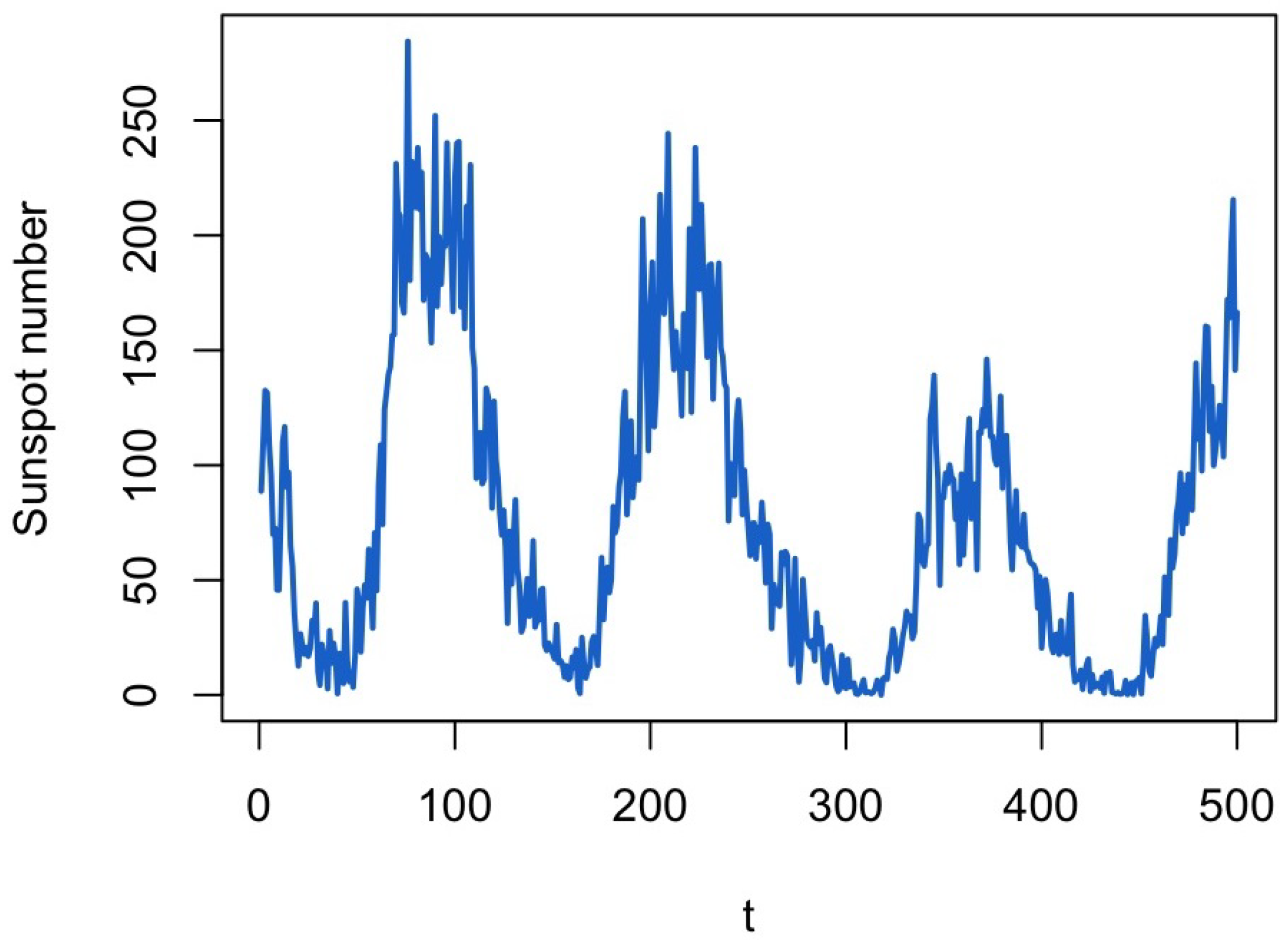
Monthly sunspot numbers were obtained from the built-in sunspot.month dataset in R (version 4.5.1), originally compiled by the World Data Center SILSO, Royal Observatory of Belgium, Brussels. The most recent 500 monthly observations (approximately 41 years) were used for this analysis (Figure 15). Table 6 reports the descriptive statistics of the series.
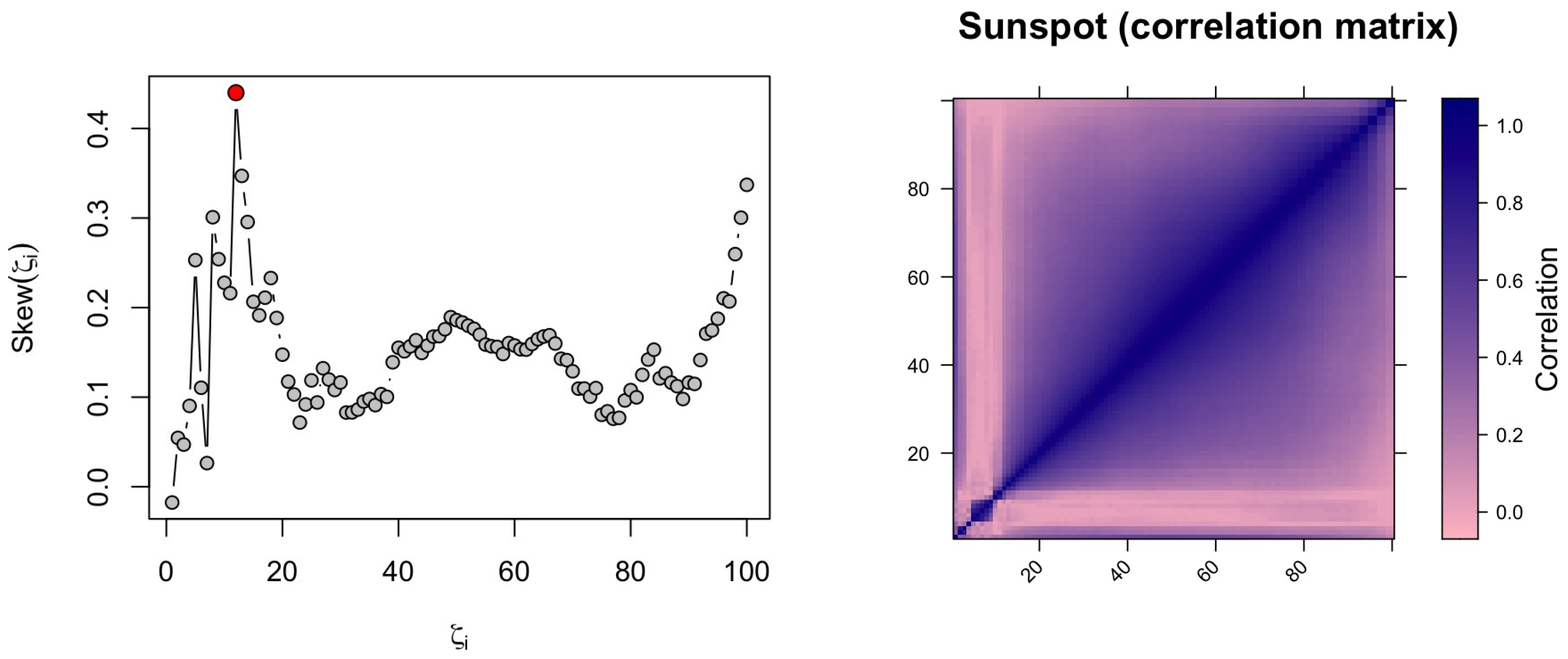
Following the same procedure applied to the COVID-19 case series, the proposed simulation-based framework was applied using a window length of L = 100 , with m = 5000 independent simulated realisations. Consistent with the criterion applied to the real-world COVID-19 data, r was selected based on the skewness of the simulated eigenvalue distributions together with the Spearman correlation structure between the eigenvalues (Figure 16). The skewness attained its highest value at ζ c = 12 , and the correlation structure similarly indicated a corresponding boundary, jointly indicating r = 11 .
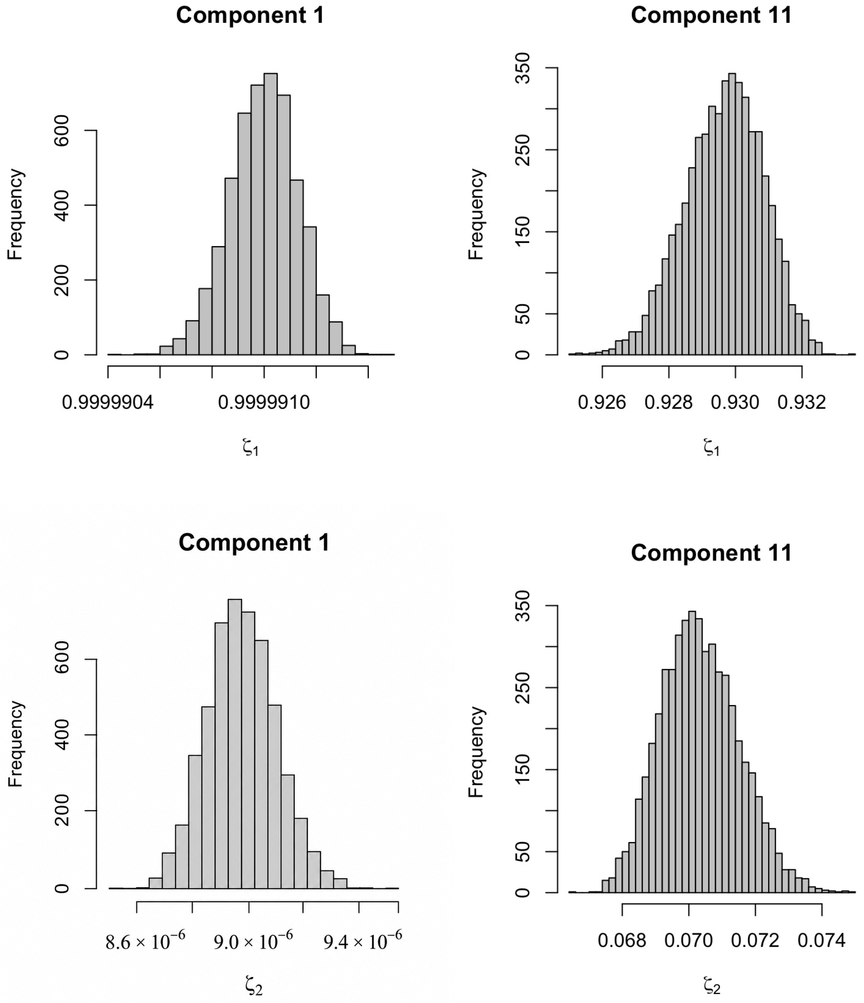
To further examine the reconstructed temporal structure, two representative components were analysed individually: Component 1 (dominant signal component) and Component 11 (the last component within the selected signal space). For each component, the eigenvalue simulation procedure applied to the KSA and UK data was repeated ( L = 2 , m = 5000 ), and the empirical distributions of ζ 1 and ζ 2 were examined (Figure 17). Both components exhibited approximately symmetric, unimodal distributions for ζ 1 and ζ 2 , consistent with their classification as part of the identified signal space, in contrast to the markedly skewed distributions characteristic of pure white-noise components observed elsewhere in this study.
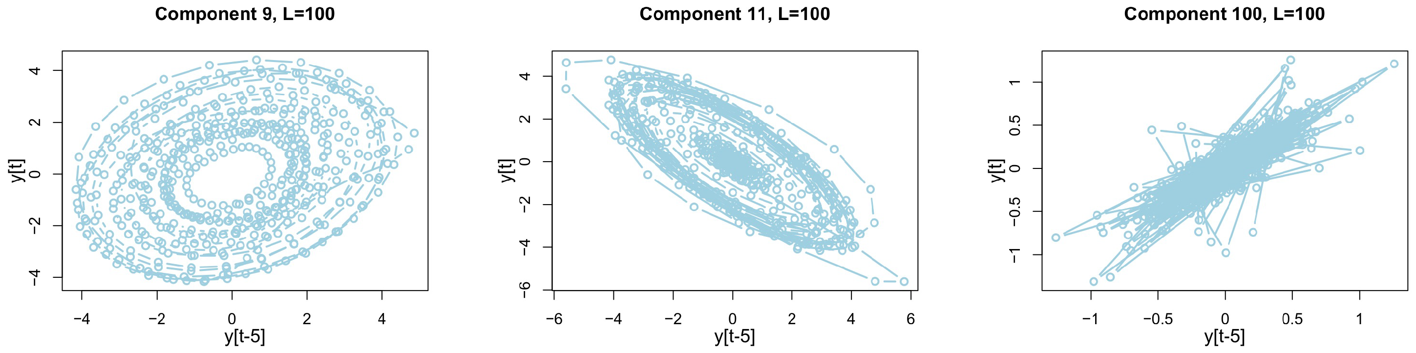
Component 9, Component 11 (the last component within the selected signal space), and the final component (Component 100, corresponding to the smallest eigenvalue) were further examined using time-delay embedding at a delay of 5 months to assess whether reconstructed components displayed attractor-like structure. Component 9 exhibited a coherent, nested spiral pattern of concentric orbits, consistent with a bounded attractor-like structure rather than random variability (Figure 18 (left)). Component 11, at the last component within the selected signal space, displayed a comparatively less sharply defined but still bounded elliptical pattern, consistent with its position at the margin of the identified signal space (Figure 18 (middle)). By contrast, Component 100, the final and smallest component in the decomposition, exhibited a diffuse and loosely scattered pattern, consistent with stochastic variability (Figure 18 (right)).
These findings are consistent with the interpretation that the sunspot series exhibits structured nonlinear temporal behaviour distinguishable from purely stochastic variability, in line with previous reports of low-dimensional structure in solar activity data [46,47]. Consistent with the cautious interpretive stance adopted throughout this study, these results are presented as evidence of finite-time statistical signatures consistent with structured nonlinear behaviour, rather than as formal proof of deterministic chaos, an issue that remains actively debated in the solar-physics literature [48]. This application illustrates that the proposed framework is readily applicable to noisy, real-world observational time series beyond epidemiological surveillance data.

5. Conclusions

This study presented a modified Singular Spectrum Analysis (SSA) framework for investigating structured nonlinear temporal behaviour in noisy observational time series and illustrated its applicability using representative COVID-19 case series from the UK and KSA, together with an independent application to monthly sunspot numbers. The proposed approach characterised dominant temporal components relative to stochastic variability, estimated an appropriate reconstruction value of r, simulated each component, and compared empirical eigenvalue distributions with those from nonlinear benchmark systems and white-noise processes. The results demonstrate the capability of the proposed framework to characterise complex temporal patterns consistent with structured nonlinear dynamics and chaotic-like behaviour over finite observational intervals.
A direct comparison with standard SSA criteria was conducted using a noisy Rössler benchmark with a known three-dimensional state-space structure. The conventional w-correlation and log-eigenvalue scree criteria identified r = 2 , whereas the proposed simulation-based framework identified r = 3 . These findings illustrate that the approaches may provide complementary characterisations of component structure under the same noisy benchmark setting, reflecting their different methodological criteria.
The observed attractor-like structures reconstructed from the COVID-19 components suggest bounded and structured temporal behaviour within the analysed time intervals. From an epidemiological perspective, exploring structured nonlinear temporal behaviour may provide complementary insight into epidemic variability, temporal instability, and short-term changes in observed epidemic patterns.
The proposed framework is readily applicable to a broad range of noisy observational time series beyond the COVID-19 case studies considered here, as demonstrated by its additional application to monthly sunspot numbers, an independent series with the long-standing and unresolved literature on nonlinear and chaotic dynamics. The framework identified structured nonlinear temporal signatures in this series consistent with previous reports in the solar-physics literature, illustrating its applicability outside the epidemiological domain. Although the present work focuses primarily on epidemiological surveillance data, the methodology is equally applicable to other domains in which complex temporal behaviour is observed under noisy conditions.
The present study extends previous SSA-based approaches by integrating simulation-based eigenvalue distribution analysis within a general time-series analysis framework, illustrated using epidemiological and solar activity case studies, together with a direct comparison with standard SSA criteria on a synthetic benchmark system. While SSA and related approaches have been applied to infectious disease dynamics and nonlinear benchmark systems, the use of simulation-based eigenvalue distribution analysis in this context remains relatively limited. The proposed framework provides a complementary nonparametric approach for exploring structured nonlinear temporal patterns and complex variability in noisy observational time series.

Supplementary Materials

The following supporting information can be downloaded at https://www.mdpi.com/article/10.3390/stats9050086/s1: processed datasets and R scripts used for the analyses and simulations.

Funding

This research received no external funding.

Institutional Review Board Statement

Not applicable.

Informed Consent Statement

Not applicable.

Data Availability Statement

The COVID-19 datasets analysed in this study are publicly available. Confirmed COVID-19 cases for the Kingdom of Saudi Arabia were obtained from the WHO COVID-19 Dashboard [44]. Confirmed COVID-19 cases for the United Kingdom were obtained from the UK Government Coronavirus Dashboard [45]. The monthly sunspot data were obtained from the sunspot.month dataset distributed with R, originally compiled by the World Data Center SILSO, Royal Observatory of Belgium. The processed datasets and the R scripts used for the analyses and simulations are provided in the Supplementary Materials.

Conflicts of Interest

The author declares no conflicts of interest.

References

  1. Ellner, S.; Turchin, P. Chaos in a Noisy World: New Methods and Evidence from Time-Series Analysis. Am. Nat. 1995, 145, 343–375. [Google Scholar] [CrossRef] [Scilit] [PubMed]
  2. Turchin, P. Complex Population Dynamics; Princeton University Press: Princeton, NJ, USA, 2013. [Google Scholar]
  3. Ellner, S.; Turchin, P. When can noise induce chaos and why does it matter: A critique. Oikos 2005, 111, 620–631. [Google Scholar] [CrossRef] [Scilit]
  4. Lorenz, E.N. Deterministic nonperiodic flow. J. Atmos. Sci. 1963, 20, 130–141. [Google Scholar] [CrossRef] [Scilit]
  5. Boeing, G. Visual analysis of nonlinear dynamical systems: Chaos, fractals, self-similarity and the limits of prediction. Systems 2016, 4, 37. [Google Scholar] [CrossRef] [Scilit]
  6. Sugihara, G.; May, R.M. Nonlinear forecasting as a way of distinguishing chaos from measurement error in time series. Nature 1990, 344, 734–741. [Google Scholar] [CrossRef] [Scilit] [PubMed]
  7. Böttcher, F.; Peinke, J.; Kleinhans, D.; Friedrich, R.; Lind, P.G.; Haase, M. Reconstruction of complex dynamical systems affected by strong measurement noise. Phys. Rev. Lett. 2006, 97, 090603. [Google Scholar] [CrossRef] [Scilit] [PubMed]
  8. Friedrich, R.; Siegert, S.; Peinke, J.; Siefert, M.; Lindemann, M.; Raethjen, J.; Deuschl, G.; Pfister, G. Extracting model equations from experimental data. Phys. Lett. A 2000, 271, 217–222. [Google Scholar] [CrossRef] [Scilit]
  9. Gao, J.B.; Hwang, S.K.; Liu, J.M. When can noise induce chaos? Phys. Rev. Lett. 1999, 82, 1132–1135. [Google Scholar] [CrossRef] [Scilit]
  10. Hudson, J.; Mankin, J. Chaos in the Belousov–Zhabotinskii reaction. J. Chem. Phys. 1981, 74, 6171–6177. [Google Scholar] [CrossRef] [Scilit]
  11. Kaplan, D.T.; Clay, J.R.; Manning, T.; Glass, L.; Guevara, M.R.; Shrier, A. Subthreshold dynamics in periodically stimulated squid giant axons. Phys. Rev. Lett. 1996, 76, 4074. [Google Scholar] [CrossRef] [Scilit] [PubMed]
  12. Hénon, M. A Two-Dimensional Mapping with a Strange Attractor. Commun. Math. Phys. 1976, 50, 69–77. [Google Scholar] [CrossRef] [Scilit]
  13. Alligood, K.T.; Sauer, T.D.; Yorke, J.A. Chaos: An Introduction to Dynamical Systems; Springer: New York, NY, USA, 1996. [Google Scholar]
  14. Wagner, J.; Bauer, S.; Contreras, S.; Fleddermann, L.; Parlitz, U.; Priesemann, V. Societal self-regulation induces complex infection dynamics and chaos. Phys. Rev. Res. 2025, 7, 013308. [Google Scholar] [CrossRef] [Scilit]
  15. Wolf, A.; Swift, J.B.; Swinney, H.L.; Vastano, J.A. Determining Lyapunov exponents from a time series. Phys. D Nonlinear Phenom. 1985, 16, 285–317. [Google Scholar] [CrossRef] [Scilit]
  16. Grassberger, P.; Procaccia, I. Measuring the strangeness of strange attractors. Phys. D 1983, 9, 189–208. [Google Scholar] [CrossRef] [Scilit]
  17. Casdagli, M. Nonlinear prediction of chaotic time series. Phys. D Nonlinear Phenom. 1989, 35, 335–356. [Google Scholar] [CrossRef] [Scilit]
  18. Kulp, C.; Zunino, L. Discriminating chaotic and stochastic dynamics through the permutation spectrum test. Chaos Interdiscip. J. Nonlinear Sci. 2014, 24, 033116. [Google Scholar] [CrossRef] [Scilit] [PubMed]
  19. Gottwald, G.A.; Melbourne, I. A new test for chaos in deterministic systems. Proc. R. Soc. Lond. Ser. A Math. Phys. Eng. Sci. 2004, 460, 603–611. [Google Scholar] [CrossRef] [Scilit]
  20. Eckmann, J.P.; Ruelle, D. Fundamental limitations for estimating dimensions and Lyapunov exponents in dynamical systems. Phys. D Nonlinear Phenom. 1992, 56, 185–187. [Google Scholar] [CrossRef] [Scilit]
  21. Gao, J.; Hu, J.; Mao, X.; Tung, W.W. Detecting low-dimensional chaos by the “noise titration” technique: Possible problems and remedies. Chaos Solitons Fractals 2012, 45, 213–223. [Google Scholar] [CrossRef] [Scilit]
  22. Proverbio, D.; Kemp, F.; Magni, S.; Gonçalves, J. Performance of early warning signals for disease re-emergence: A case study on COVID-19 data. PLoS Comput. Biol. 2022, 18, e1009958. [Google Scholar] [CrossRef] [Scilit] [PubMed]
  23. Lacasa, L.; Toral, R. Description of stochastic and chaotic series using visibility graphs. Phys. Rev. E 2010, 82, 036120. [Google Scholar] [CrossRef] [Scilit] [PubMed]
  24. Toker, D.; Sommer, F.T.; D’Esposito, M. A simple method for detecting chaos in nature. Commun. Biol. 2020, 3, 11. [Google Scholar] [CrossRef] [Scilit] [PubMed]
  25. Mangiarotti, S.; Peyre, M.; Zhang, Y.; Huc, M.; Roger, F.; Kerr, Y. Chaos theory applied to the outbreak of COVID-19: An ancillary approach to decision making in pandemic context. Epidemiol. Infect. 2020, 148, e95. [Google Scholar] [CrossRef] [Scilit] [PubMed]
  26. Al-Turaiki, I.; Almutlaq, F.; Alrasheed, H.; Alballa, N. Empirical Evaluation of Alternative Time-Series Models for COVID-19 Forecasting in Saudi Arabia. Int. J. Environ. Res. Public Health 2021, 18, 8660. [Google Scholar] [CrossRef] [Scilit] [PubMed]
  27. Awwad, F.; Mohamoud, M.; Abonazel, M. Estimating COVID-19 cases in Makkah region of Saudi Arabia: Space-time ARIMA modeling. PLoS ONE 2021, 16, e0250149. [Google Scholar] [CrossRef] [Scilit] [PubMed]
  28. Youssef, H.; Alghamdi, N.; Ezzat, M.; El-Bary, A.; Shawky, A. A proposed modified SEIQR epidemic model to analyze the COVID-19 spreading in Saudi Arabia. Alex. Eng. J. 2021, 61, 2456–2470. [Google Scholar] [CrossRef] [Scilit]
  29. Ghodsi, Z.; Silva, E.S.; Hassani, H. Bicoid signal extraction with a selection of parametric and nonparametric signal processing techniques. Genom. Proteom. Bioinform. 2015, 13, 183–191. [Google Scholar] [CrossRef] [Scilit] [PubMed]
  30. Sanei, S.; Hassani, H. Singular Spectrum Analysis of Biomedical Signals; CRC Press: Boca Raton, FL, USA, 2015. [Google Scholar] [CrossRef] [Scilit]
  31. Muruganatham, B.; Sanjith, M.; Krishnakumar, B.; Murty, S.S. Roller element bearing fault diagnosis using singular spectrum analysis. Mech. Syst. Signal Process. 2013, 35, 150–166. [Google Scholar] [CrossRef] [Scilit]
  32. Hassani, H.; Rua, A.; Silva, E.S.; Thomakos, D. Monthly forecasting of GDP with mixed-frequency multivariate singular spectrum analysis. Int. J. Forecast. 2019, 35, 1263–1272. [Google Scholar] [CrossRef] [Scilit]
  33. Kalantari, M. Forecasting COVID-19 pandemic using optimal singular spectrum analysis. Chaos Solitons Fractals 2021, 142, 110547. [Google Scholar] [CrossRef] [Scilit] [PubMed]
  34. Broomhead, D.; King, G. Extracting qualitative dynamics from experimental data. Phys. D 1986, 20, 217–236. [Google Scholar] [CrossRef] [Scilit]
  35. Golyandina, N.; Nekrutkin, V.; Zhigljavsky, A.A. Analysis of Time Series Structure: SSA and Related Techniques, 1st ed.; Chapman and Hall/CRC: Boca Raton, FL, USA, 2001. [Google Scholar] [CrossRef] [Scilit]
  36. Golyandina, N.; Zhigljavsky, A. Singular Spectrum Analysis for Time Series; Springer Briefs in Statistics; Springer: Berlin/Heidelberg, Germany, 2013. [Google Scholar]
  37. Hassani, H.; Alharbi, N.; Ghodsi, M. Distinguishing chaos from noise: A new approach. Int. J. Energy Stat. 2014, 2, 137–150. [Google Scholar] [CrossRef] [Scilit]
  38. Alharbi, N.; Hassani, H. A new approach for selecting the number of the eigenvalues in singular spectrum analysis. J. Frankl. Inst. 2016, 353, 1–16. [Google Scholar] [CrossRef] [Scilit]
  39. Alharbi, N. A novel approach for noise removal and distinction of EEG recordings. Biomed. Signal Process. Control 2018, 39, 23–33. [Google Scholar] [CrossRef] [Scilit]
  40. Kantz, H.; Schreiber, T. Nonlinear Time Series Analysis, 2nd ed.; Cambridge University Press: Cambridge, UK, 2010. [Google Scholar] [CrossRef] [Scilit]
  41. Hassani, H.; Alharbi, N.; Ghodsi, M. A study on the empirical distribution of the scaled Hankel matrix eigenvalues. J. Adv. Res. 2015, 6, 925–929. [Google Scholar] [CrossRef] [Scilit] [PubMed]
  42. Alharbi, N. Forecasting the COVID-19 Pandemic in Saudi Arabia Using a Modified Singular Spectrum Analysis Approach: Model Development and Data Analysis. JMIRx Med 2021, 2, e21044. [Google Scholar] [CrossRef] [Scilit] [PubMed]
  43. D’Agostino, R.B. Goodness-of-Fit-Techniques; CRC Press: Boca Raton, FL, USA, 1986; Volume 68. [Google Scholar]
  44. World Health Organization. WHO COVID-19 Dashboard: Saudi Arabia; World Health Organization: Geneva, Switzerland, 2021. [Google Scholar]
  45. UK Government. Coronavirus (COVID-19) in the UK; UK Government: London, UK, 2021.
  46. Pavlos, G.P.; Dialetis, D.; Kyriakou, G.A.; Sarris, E.T. A preliminary low-dimensional chaotic analysis of the solar cycle. Ann. Geophys. 1992, 10, 759. [Google Scholar]
  47. Letellier, C.; Aguirre, L.A.; Maquet, J.; Gilmore, R. Evidence for low dimensional chaos in sunspot cycles. Astron. Astrophys. 2006, 449, 379–387. [Google Scholar] [CrossRef] [Scilit]
  48. Panchev, S.; Tsekov, T. Empirical evidences of persistence and dynamical chaos in solar terrestrial phenomena. J. Atmos. Sol.-Terr. Phys. 2007, 69, 2391–2404. [Google Scholar] [CrossRef] [Scilit]
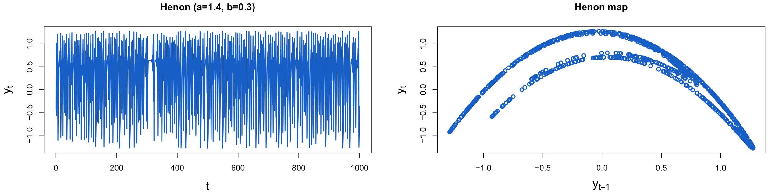
Figure 1. Illustrative Hénon time series (left) and the corresponding phase-space attractor (right), demonstrating how an apparently irregular temporal sequence gives rise to a structured nonlinear attractor.
Stats 09 00086 g001
Figure 2. Logarithm of the mean eigenvalues, ζ ¯ i , for the noisy Rössler time series, illustrating the dominance of the first three components.
Stats 09 00086 g002
Figure 3. Skewness (top left), kurtosis (top right), coefficient of variation (bottom left), and the absolute Spearman correlation matrix (bottom right) of the eigenvalues for the noisy Rössler time series.
Stats 09 00086 g003
Figure 4. Standard SSA diagnostics for the noisy Rössler series: log-eigenvalue ( λ i ) scree plot, showing the classical elbow at r = 2 , with the red point indicating the selected elbow (left), and the w-correlation matrix of reconstructed components, showing grouping into a dominant two-component block (right).
Stats 09 00086 g004
Figure 5. Histograms of ζ i = 1 , 2 for the white-noise process (top) and the Hénon time series (bottom).
Stats 09 00086 g005
Figure 6. Spearman correlation matrices of ζ i , j = 1 , , 10 for the white-noise process (left) and the Hénon time series (right).
Stats 09 00086 g006
Figure 7. Daily reported COVID-19 cases for the KSA (left) and the UK (right).
Stats 09 00086 g007
Figure 8. Absolute Spearman correlations between consecutive eigenvalues ζ i and ζ i + 1 ( i = 1 , , 6 ) (left), with the red point indicating the minimum correlation used to identify the signal–noise boundary at r = 2 , and the absolute Spearman correlation matrix of ζ i and ζ j ( i , j = 1 , , 7 ) (right) for the KSA COVID-19 data.
Stats 09 00086 g008
Figure 9. Histograms of ζ i = 1 , 2 for the reconstructed components with L = 2 from the KSA COVID-19 case series. Component 1 is shown in the top row and Component 2 in the bottom row; ζ 1 is shown in the left column and ζ 2 in the right column.
Stats 09 00086 g009
Figure 10. Histograms of ζ i = 1 , 2 for the reconstructed third to seventh components with L = 7 from the KSA COVID-19 case series.
Stats 09 00086 g010
Figure 11. Histograms of ζ i = 1 , 2 for the reconstructed smallest, middle, and largest components with L = 100 from the KSA COVID-19 case series.
Stats 09 00086 g011
Figure 12. Histograms of ζ i = 1 , 2 for the reconstructed smallest, middle, and largest components with L = 100 from the UK COVID-19 case series.
Stats 09 00086 g012
Figure 13. Results for the KSA COVID-19 data. The scatter plot of y t with a time delay of one reveals a pattern for the second component when L = 7 (left). An attractor-like pattern (orbit) from the fifth component when L = 100 is observed, showcasing its dynamic range (right).
Stats 09 00086 g013
Figure 14. Results for the UK COVID-19 data when L = 100 . Attractor-like patterns were observed in the third, fourth, and sixth components under different time-delay settings.
Stats 09 00086 g014
Figure 15. Monthly sunspot numbers (most recent 500 months) used in this analysis.
Stats 09 00086 g015
Figure 16. Skewness (left), with the red point indicating the maximum skewness at ζ c = 12 , and the absolute Spearman correlation matrix (right) of the eigenvalues for the sunspot series.
Stats 09 00086 g016
Figure 17. Histograms of ζ 1 (top row) and ζ 2 (bottom row) for Component 1 (left) and Component 11, the last component within the selected signal space (right) for the sunspot number series.
Stats 09 00086 g017
Figure 18. Time-delay embedding at a delay of 5 months for Component 9 (left); Component 11, the last component within the selected signal space (middle); and Component 100 (right) for the sunspot number series.
Stats 09 00086 g018
Table 1. Comparison between standard SSA and the proposed modified SSA framework.
FeatureStandard SSAProposed Modified SSA Framework
ObjectiveSignal decomposition and reconstruction.Signal decomposition followed by simulation-based investigation of structured nonlinear temporal behaviour.
Eigenvalue analysisUses the eigenspectrum for component ranking and signal reconstruction.Uses simulation-based empirical eigenvalue distributions to characterize both the original series and the reconstructed components.
Selection of rBased mainly on the eigenspectrum and component separability.Based on statistical properties of simulated eigenvalue distributions, including skewness, kurtosis, coefficient of variation, and eigenvalue correlations.
Analysis of reconstructed componentsComponents are reconstructed to recover the underlying signal.Each reconstructed component is analysed individually using the proposed simulation framework, and its empirical eigenvalue distributions are compared with white-noise processes and canonical nonlinear benchmark systems.
Additional analysisNot an intrinsic component of the standard SSA procedure.Time-delay embedding and phase-space reconstruction are used to investigate bounded attractor-like temporal patterns.
Table 2. Comparison of standard SSA criteria and the proposed method for selecting r on the noisy Rössler benchmark.
MethodBasisSelected r
W-correlationStandard SSA: weighted correlation between reconstructed components [36]2
Log-eigenvalue scree plotStandard SSA: classical elbow in the log-singular-value spectrum2
Proposed methodSimulation-based skewness, kurtosis, CV, and correlation diagnostics3
Table 3. Coefficients of skewness for ζ i = 1 , 2 for the white-noise process and the Hénon time series.
Coefficient of Skewness of ζ i
WN Hénon
ζ 1 0.99−0.034
ζ 2 −0.990.034
Table 4. D–P test P-values for ζ i = 1 , 2 for the white-noise process and the Hénon time series.
D–P Test p-Values for ζ i
WN Hénon
ζ 1 < 0.01 0.2
ζ 2 < 0.01 0.2
Table 5. Descriptive statistics of the original daily COVID-19 case series.
DatasetLength (Days)MeanMedianStd. Dev.IQRMin–MaxSkewnessKurtosis
UK54710,693.42428613,892.091514.50–81,5031.903.83
KSA402984.71423.51106.511340–49191.541.51
Table 6. Descriptive statistics of the sunspot number series analysed.
DatasetLength (Months)MeanMedianStd. Dev.IQRMin–MaxSkewnessKurtosis
Sunspots50075.7660.964.7397.350–284.50.80−0.29
Disclaimer/Publisher’s Note: The statements, opinions and data contained in all publications are solely those of the individual author(s) and contributor(s) and not of MDPI and/or the editor(s). MDPI and/or the editor(s) disclaim responsibility for any injury to people or property resulting from any ideas, methods, instructions or products referred to in the content.