Central Limit Theorem of the Recursive Estimate of Density Function Under Randomly Censored Data

Abstract

Kernel density estimation for right-censored data has been extensively studied in the non-recursive setting, whereas recursive approaches adapted to censoring remain largely unexplored despite their considerable computational advantages in sequential data environments. In this paper, we introduce a recursive kernel density estimator for independent right-censored observations through a Kaplan-Meier weighting scheme. The proposed estimator can be updated incrementally as new observations become available, avoiding repeated re-computation of the entire estimator and substantially reducing memory and computational requirements. Under mild regularity conditions, we establish the asymptotic normality of the estimator and derive its asymptotic variance, which explicitly reflects the effect of the recursive weighting mechanism and the censoring process. We also construct asymptotic confidence intervals for the underlying density using a plug-in variance estimator. An extensive Monte Carlo study, including Gaussian, exponential, heavy-tailed, multimodal, contaminated, and severely censored scenarios, demonstrates that the proposed estimator achieves estimation accuracy comparable to that of the classical censored Parzen-Rosenblatt estimator while offering substantial computational gains. In particular, the recursive procedure remains stable under high censoring levels and exhibits excellent scalability for large and sequentially collected datasets. The proposed methodology provides an efficient and theoretically justified alternative for nonparametric density estimation under right censoring and is particularly suited to applications involving streaming data, such as survival analysis, reliability engineering, medical monitoring, and online forecasting.

1. Introduction

Nonparametric kernel estimation has been extensively studied under a variety of data assumptions, including independent or dependent structures and complete or incomplete observations. This estimation framework provides a useful means to model the uncertainty inherent in forecasting problems.

Among the foundational works, the kernel density estimator was first introduced by Rosenblatt [1] for independent and fully observed data. However, in many real-world situations, such as clinical trials or reliability studies, the data collected are often subject to censoring, meaning that the variable of interest is not always fully observed.

Consequently, significant attention has been devoted to nonparametric estimation under censored models. For instance, Diehl and Stute [2] studied the consistency of density and hazard function estimators for independent right-censored data, Mielniczuk [3] established the asymptotic normality of a density estimator in the right-censored case and Boukeloua and Messaci [4] further explored asymptotic normality under general censoring conditions. Many authors (see e.g., Carbonez el al. [5], Kohler et al. [6], Guessoum and Ould-Saïd [7,8,9], Ould Saïd and Cai [10] and Ould Saïd [11] among others) use the so-called synthetic data which allow to take into account the censoring effect on the lifetime distribution. Lemdani and Ould Saïd [12] established the uniform consistency with rate and asymptotic normality for the estimators using the Vapnik-Chervonenkis class (VC class) under i.i.d right censored data.

The literature on non-parametric functional estimation under incomplete observations has been extensively enriched by the pioneering contributions of Ould-Saïd and collaborators (see, e.g., Ould-Saïd et al. [13,14,15]). This prominent line of research focused heavily on exploring the asymptotic refinements, uniform consistency, and general applicability of kernel density and conditional hazard estimators under censorship or truncation, frequently operating within complex dependence frameworks such as $\alpha$-mixing or ergodic processes.

However, a fundamental operational paradigm shared across these foundational works is their strict reliance on non-recursive kernel methods. In classical non-recursive estimation, the arrival of any incremental data point necessitates storing the entire historical trajectory and re-evaluating the global sum from scratch, inducing a cumulative memory and computational burden of $\mathcal{O}\left(n\right)$.

The objective of this manuscript is to bridge this operational gap by developing and analyzing a recursive kernel density estimator specifically tailored for right-censored independent data. Unlike historical non-recursive frameworks, the proposed estimator utilizes a step-by-step incremental update strategy based on sequential Kaplan-Meier survival weights. This design reduces the update complexity per new observation to $\mathcal{O}\left(1\right)$.

We establish its full asymptotic normality under mild, standard regularity conditions and explicitly demonstrate its distinct computational advantages. Consequently, this study shifts the focus from static batch processing toward high-frequency, stream-based survival analysis architectures, providing a defensible added value to the nonparametric framework established by prior authors.

Recursivity is a powerful technical tool in estimation, offering the advantage of updating estimators incrementally without recomputing from scratch. This approach significantly reduces computational time and memory usage, particularly when handling large datasets arriving sequentially.

In the context of independent and $\alpha$-mixing complete data, Amiri [16] introduced and analyzed a family of recursive estimators, which includes earlier versions proposed by Deheuvels [17] and Wegman and Davies [18]. Later, Mezhoud et al. [19] extended this work to the case of weakly dependent complete data.

However, since the variable of interest is often not entirely observable in practice, this study focuses on censored data. To the best of our knowledge, the recursive estimator generalized by Amiri [16] has not yet been investigated within a censored data framework.

In this work, we introduce in Section 2 a right-censoring model and propose a recursive estimator based on the Kaplan-Meier estimator (Kaplan and Meier [20]). Section 3 presents the basic assumptions and establishes the asymptotic convergence in distribution to a normal law for the proposed recursive estimator. Finally, Section 4 is dedicated to a simulation study assessing the performance and computational efficiency of our estimator.

The primary motivation for introducing recursion in the censored-data framework is not to replace existing kernel density estimators, but rather to provide a computationally efficient alternative for settings where observations become available sequentially. Classical kernel density estimators adapted to censoring are typically computed from the entire sample whenever new observations are added. Consequently, the computational burden increases rapidly with the sample size, making repeated estimation costly in large-scale applications.

In contrast, the recursive estimator proposed in this work can be updated incrementally as new censored observations arrive. The recursive representation avoids recomputing the complete estimator from scratch and only requires the previous estimate together with the incoming observation. This feature substantially reduces computational effort and memory requirements, particularly when the data are collected continuously over time. Such situations arise naturally in survival analysis, reliability engineering, medical monitoring, industrial quality control, and online forecasting systems, where lifetimes or event times are progressively recorded and immediate updates of the estimated density are desirable. In these contexts, recursive procedures offer an attractive compromise between statistical accuracy and computational efficiency.

From a theoretical perspective, establishing asymptotic normality under right censoring is essential because it guarantees that the computational gains obtained through recursion do not come at the expense of asymptotic statistical validity. Therefore, the contribution of this paper should be viewed as extending the recursive estimation paradigm to censored data while preserving the classical asymptotic properties required for statistical inference.

2. Model and Estimator

Let us consider T be a positive lifetime variable with continuous distribution function F and an unknown density f.

Recall that, in the complete data case, Amiri [16] defined the family of recursive estimates as

$${\displaystyle {\overline{f}}_n^{\ell }\left(t\right)=\frac{1}{{\sum }_{i=1}^n{h}_i^{1-\ell }}{\displaystyle \sum _{i=1}^n}\frac{1}{h_i^{\ell }}K\left(\frac{t-T_i}{h_i}\right),t\in \mathbb{R},}$$

(1)

where $\left(h_n\right)$ is a positive bandwidth sequence decreasing to zero, K is a kernel density, and $\ell \in [0,1]$ is a smoothing parameter, it is considered here to obtain a more general estimator.

Let ${\left(T_i\right)}_{1\le i\le n}$ be a sequence of independent and identically distributed lifetime random variables with continuous distribution function F and density f. In practice, lifetimes are often incompletely observed because of censoring; and let $\left(C_i\right)1\le i\le n$ be a sequence of independent censoring variables with distribution function G and survival function $\overline{G}=1-G$. We assume that $\left(T_i\right)$ and $\left(C_i\right)$ are mutually independent. Instead of observing $T_i$, we observe the pairs ${(Y_i,{\delta }_i)}_{i=1,\dots ,n}$, where $Y_i=min(T_i,C_i)$ and ${\delta }_i={\mathbb{I}}_{T_i\le C_i}.$

Thus, ${\delta }_i=0$ indicates an uncensored observation, whereas ${\delta }_i=1$ corresponds to a censored observation.

Since $\mathbb{E}({\delta }_i\mid T_i)=1-G\left(T_i\right)=\overline{G}\left(T_i\right)$, so for $i=1,\dots ,n$, we have

$$\mathbb{E}\left[K\left({\displaystyle \frac{t-Y_i}{h_i}}\right){\displaystyle \frac{{\delta }_i}{\overline{G}\left(Y_i\right)}}\right]=\mathbb{E}\left[K\left({\displaystyle \frac{t-T_i}{h_i}}\right)\right].$$

Consequently from estimator given by (1), we first construct the estimator

$${\tilde{f}}_n^{\ell }\left(t\right)={\displaystyle \frac{1}{{\sum }_{i=1}^n{h}_i^{1-\ell }}}{\displaystyle \sum _{i=1}^n}{\displaystyle \frac{1}{h_i^{\ell }}}K\left({\displaystyle \frac{t-Y_i}{h_i}}\right){\displaystyle \frac{{\delta }_i}{\overline{G}\left(Y_i\right)}}.$$

(2)

The cumulative distribution function G, of the censoring random variables, is estimated by Kaplan and Meier [20] estimator defined as follows

$$\begin{array}{c}\hfill {\overline{G}}_n\left(t\right)=1-G_n\left(t\right)=\left\{\begin{array}{cc}{\displaystyle {\prod }_{i=1}^n}{\left(1-{\displaystyle \frac{1-{\delta }_{\left(i\right)}}{n-i+1}}\right)}^{{\mathbb{I}}_{\{Y_{\left(i\right)}\le t\}}}\hfill & \mathrm{if}t<Y_{\left(n\right)},\hfill \\ 0\hfill & \mathrm{Otherwise},\hfill \end{array}\right.\end{array}$$

where $(Y_{\left(i\right)},{\delta }_{\left(i\right)})$ are the n ordered pairs in $Y_i$. Here ${\delta }_{\left(i\right)}$ is the concomitant of $Y_{\left(i\right)}$.

We introduce finally our recursive kernel estimator adapted to right-censored data

$$f_n^{\ell }\left(t\right)={\displaystyle \frac{1}{{\sum }_{i=1}^n{h}_i^{1-\ell }}}{\displaystyle \sum _{i=1}^n}{\displaystyle \frac{1}{h_i^{\ell }}}K\left({\displaystyle \frac{t-Y_i}{h_i}}\right){\displaystyle \frac{{\delta }_i}{{\overline{G}}_n\left(Y_i\right)}}.$$

(3)

Note that for a sample of complete data $({\delta }_{\left(i\right)}=0,\forall i=1,\dots ,n)$. The estimator (3) is similar in this case to the estimator introduced by Amiri [16].

Unlike (Rosenblatt [1]) estimator, the recursive form (3) allows updating the estimate without recalculating all the data as new observations arrive. Indeed, the estimator (3) satisfies the recursion

$$f_{n+1}^{\ell }\left(t\right)={\displaystyle \frac{{\sum }_{i=1}^n{h}_i^{1-\ell }}{{\sum }_{i=1}^{n+1}{h}_i^{1-\ell }}}{f}_n^{\ell }\left(t\right)+{\displaystyle \frac{1}{{\sum }_{i=1}^{n+1}{h}_i^{1-\ell }}}{\displaystyle \frac{1}{h_{n+1}^{\ell }}}K\left({\displaystyle \frac{t-Y_{n+1}}{h_{n+1}}}\right){\displaystyle \frac{{\delta }_{n+1}}{{\overline{G}}_n\left(Y_{n+1}\right)}}.$$

(4)

with $K_{n+1}(t-Y_{n+1})={\displaystyle \frac{1}{h_{n+1}^{\ell }}}K\left({\displaystyle \frac{t-Y_{n+1}}{h_{n+1}}}\right)$.

3. Asymptotic Study

In this section, the asymptotic normality of the estimator defined in (3) is established here. In our analysis, the following assumptions will be used.

3.1. Main Result

(H1)

$n{h}_n^3\to 0$ and $n{h}_n^5=\mathcal{O}\left(1\right)$ as $n\to \infty$.

(H2)

${\beta }_{n,r}={\displaystyle \frac{1}{n}}{\sum }_{i=1}^n{(h_i/h_n)}^r\to {\beta }_r<\infty$ as $n\to \infty ,r\le 3$.

(H3)

$h_n=o\left({(logn)}^{-\alpha }\right)$, $0<\alpha <1$.

(H4)

The kernel K is a positive bounded function with compact support.

(H5)

$\int vK\left(v\right)dv=0$.

(H6)

f is twice continuously differentiable on $\mathbb{R}$.

Roughly speaking, these assumptions are very standard and classically used in the nonparametric estimation. The technical conditions (H1), (H3), (H4) and (H5) are necessary for proving the results. However, the condition $n{h}_n^3\to 0$ implies that $n{h}_n\to \infty$, while the choice $h_n=C{n}^{-\gamma }$ with $\frac{1}{5}<\alpha <\gamma <\frac{1}{3}$, fulfills the assumptions (H1) and (H3). The particular recursion assumption of previously mentioned in (Yamato [21]) for $r=-1$, (Wegman and Davies [18]) for $r=\frac{1}{2}$ and in (Isogai [22]) for $r\le 0$, are essentials to smooth the complexity of calculation associated with recursive kernels. Lastly, the assumption (H6) stands as regularity condition, it permits us to evaluate the bias and the variance terms in order to obtain our results.

The quantities $\frac{1}{n}{\sum }_{i=1}^n{\left(\frac{h_i}{h_n}\right)}^r$ naturally arise from the recursive weighting mechanism. Unlike the classical kernel estimator, where all observations contribute equally, recursive estimation assigns observation-specific weights.

The limits ${lim}_{n\to \infty }{\beta }_{n,r}$ summarize the cumulative effect of recursion on the asymptotic distribution. For the commonly used bandwidth sequence $h_n=C{n}^{-\gamma },0<\gamma <1,$ one obtains $\frac{1}{1-r\gamma },$ whenever $r\gamma <1$.

Theorem 1. 

Assume that assumptions (H1)–(H6) hold. Then the sequence

$$\sqrt{n{h}_n}\left(f_n^{\ell }\left(t\right)-f\left(t\right)\right)\stackrel{\mathcal{D}}{\to }\mathcal{N}(0,{\sigma }_{\ell }^2),$$

where $\stackrel{\mathcal{D}}{\to }$ denotes the convergence in distribution and

$${\sigma }_{\ell }^2={\displaystyle \frac{{\beta }_{1-2\ell }}{{\beta }_{1-\ell }^2}}{\displaystyle \frac{f\left(t\right)}{\overline{G}\left(t\right)}}\int K^2\left(v\right)dv.$$

• Methodological Interpretation of the Normalization Factor: ${\beta }_{n,r}$.

A crucial mathematical element in the structural stability of the proposed recursive kernel estimator $f_n^{\ell }\left(t\right)$ is the sequence of normalization constants ${\beta }_{n,r}$. Assume that

$$h_n=C{n}^{-\gamma },0<\gamma <1.$$

Then

$${\beta }_{n,r}={\displaystyle \frac{1}{n}}{\displaystyle \sum _{i=1}^n}{\left({\displaystyle \frac{h_i}{h_n}}\right)}^r={\displaystyle \frac{1}{n}}{\displaystyle \sum _{i=1}^n}{\left({\displaystyle \frac{i}{n}}\right)}^{-r\gamma },$$

and

$$\underset{n\to \infty }{lim}{\beta }_{n,r}={\beta }_r={\displaystyle \frac{1}{1-r\gamma }}<\infty ,<1.$$

The constants ${\beta }_r$ measure the cumulative contribution of previous bandwidths to the recursive estimator. They characterize the memory effect introduced by recursion and directly determine the asymptotic variance.

Substituting the above expression into Theorem 1 yields

$${\displaystyle {\sigma }_{\ell }^2=\frac{{(1-(1-\ell )\gamma )}^2}{1-(1-2\ell )\gamma }\frac{f\left(t\right)}{\overline{G}\left(t\right)}\int K^2\left(u\right)du}$$

Consequently, the recursive parameter ℓ controls the trade-off between memory accumulation and estimation variability.

In order to measure relative efficiency considering the classical censored Parzen-Rosenblatt Estimator defined by

$$f_n^{PR}\left(t\right)={\displaystyle \frac{1}{n{h}_n}}{\displaystyle \sum _{i=1}^n}{\displaystyle \frac{{\delta }_i}{{\overline{G}}_n\left(Y_i\right)}}K\left({\displaystyle \frac{t-Y_i}{h_i}}\right),t\in \mathbb{R},$$

(5)

Its asymptotic variance is given by

$${\sigma }^2={\displaystyle \frac{f\left(t\right)}{\overline{G}\left(t\right)}}\int K^2\left(u\right)du,$$

the asymptotic relative efficiency of the recursive estimator is

$${\displaystyle ARE(\ell )=\frac{{\sigma }^2}{{\sigma }_{\ell }^2}=\frac{{\beta }_{1-\ell }^2}{{\beta }_{1-2\ell }}.}$$

For bandwidth sequences satisfying $h_n=C{n}^{-\gamma },$$0<\gamma <1$ one has $ARE(\ell )>1$.

Hence the recursive estimator possesses a smaller asymptotic variance than the classical censored kernel estimator.

This result shows that recursion does not merely reduce computational complexity. It also improves asymptotic efficiency through the variance reduction factor $\frac{{\beta }_{1-2\ell }}{{\beta }_{1-\ell }^2}$.

Unlike standard non-recursive Parzen-Rosenblatt estimators, where the window parameter $h_n$ remains static across the entire dataset, the recursive framework dynamically embeds the historical sequence of bandwidths ${\left(h_i\right)}_{i=1}^n$ inside the algorithmic updates. This continuous structural coupling requires an explicit regularizing sequence to ensure that early sequential data points do not distort the asymptotic properties of the estimator.

Physically, the ratio ${(h_i/h_n)}^r$ acts as a temporal weighting scheme. When the window sequence satisfies the classical optimal bias-variance criteria $h_n=C{n}^{-\gamma }$ with $\gamma \in (1/5,1/3)$, it is straightforward to prove via Riemann sum approximations that the sequence ${\beta }_{n,r}$ converges to a deterministic limit ${\beta }_r$.

In our asymptotic variance proof (Theorem 1), the compound factor $\frac{{\beta }_{1-2\ell }}{{\beta }_{1-\ell }^2}$ arises directly from this normalization mechanism. This term scales the variance under censorship according to the selected smoothing parameter ℓ. Because ${\beta }_r$ decreases regularly with n, selecting $\ell =1$ ensures that this specific compound ratio remains strictly below 1. This establishes a higher variance reduction and asymptotic efficiency compared to non-recursive configurations, directly validating the theoretical advantage of our framework in streaming survival data architectures.

Remark 1. 

1. 

Isogai [22] and Masry [23] obtained the asymptotic normality of the recursive estimator for the special cases $\ell =1,\ell =\frac{1}{2}$, with independent and α-mixing complete data. While Amiri [16] and Mezhoud et al. [19] studied the estimator (3) for α-mixing and η-dependent complete data.

2. 

Boukeloua and Messaci [4] investigated asymptotic normality in a censored model of the non-recursive density estimator

$$f_n\left(x\right)={\displaystyle \frac{1}{h_n}}\int K\left({\displaystyle \frac{x-y}{h_n}}d{F}_n\left(y\right)\right),$$

where $F_n$ is the empirical distribution function of the observed lifetime variables $T_i$ and obtained asymptotic variance ${\sigma }^2=\frac{f\left(x\right)}{\overline{G}\left(x\right)}\int K^2\left(v\right)dv$, while in Theorem 1, the variance given ${\sigma }_{\ell }^2={\sigma }^2$. Indeed, one can prove that the ratio $\frac{{\beta }_{1-2\ell }}{{\beta }_{1-\ell }^2}<1$ holds under the bandwidth choice $h_n=n^{-\frac{1}{5}}$, in other words the ratio remains below 1 when the bandwidth sequence $h_n$ satisfies the standard conditions $h_n\to 0$ and $n{h}_n\to \infty$, and decreases regularly with n (see Amiri [16]).

3. 

The asymptotic variance satisfies ${\sigma }_{\ell }^2<{\sigma }^2$ of the classical non-recursive kernel estimator, yielding improved efficiency.

Proof. 

In what follows, because ${\overline{G}}_n$ is discontinuous, we need to use the estimator (2). Our result will be obtained then from the following decomposition

$$\begin{array}{ccc}\hfill \sqrt{n{h}_n}\left(f_n^{\ell }\left(t\right)-f\left(t\right)\right)& =& \sqrt{n{h}_n}\left[\left(f_n^{\ell }\left(t\right)-{\tilde{f}}_n^{\ell }\left(t\right)\right)+\left({\tilde{f}}_n^{\ell }\left(t\right)-\mathbb{E}{\tilde{f}}_n^{\ell }\left(t\right)\right)+\left(\mathbb{E}{\tilde{f}}_n^{\ell }\left(t\right)-f\left(t\right)\right)\right]\hfill \\ & =& I_1+I_2+I_3,\hfill \end{array}$$

where ${\displaystyle {\tilde{f}}_n^{\ell }\left(t\right)=\frac{1}{{\sum }_{i=1}^n{h}_i^{1-\ell }}{\displaystyle \sum _{i=1}^n}{h}_i^{-\ell }K\left(\frac{t-Y_i}{h_i}\right)\frac{{\delta }_i}{\overline{G}\left(Y_i\right)}.}$

• Control of the first term
  Along intermediate steps of this proof we assume that $T_Y<\infty$, where $T_Y:=sup\{t,F_Y\left(t\right)<1\}$ and let $\theta$ be a positive real number such that $\theta <T_Y$ we have

  $$\begin{array}{ccc}\hfill I_1& \le & {\displaystyle \sqrt{n{h}_n}\frac{1}{{\sum }_{i=1}^n{h}_i^{1-\ell }}{\displaystyle \sum _{i=1}^n}{h}_i^{-\ell }K\left(\frac{t-Y_i}{h_i}\right)\frac{|{\overline{G}}_n\left(Y_i\right)-\overline{G}\left(Y_i\right)|}{{\overline{G}}_n\left(Y_i\right)\overline{G}\left(Y_i\right)}}\hfill \\ & \le & {\displaystyle \frac{{\displaystyle \underset{t<\theta }{sup}|{\overline{G}}_n\left(Y_i\right)-\overline{G}\left(Y_i\right)|}}{{\overline{G}}_n\left(Y_i\right)\overline{G}\left(Y_i\right)}}{\displaystyle \frac{1}{{\sum }_{i=1}^n{h}_i^{1-\ell }}}{\displaystyle \sum _{i=1}^n}{h}_i^{-\ell }K\left({\displaystyle \frac{t-Y_i}{h_i}}\right).\hfill \end{array}$$
  From (Mezhoud el al. [19]), we obtain

  $${\displaystyle \underset{n\to \infty }{lim}\frac{1}{{\sum }_{i=1}^n{h}_i^{1-\ell }}{\displaystyle \sum _{i=1}^n}{h}_i^{-\ell }K\left(\frac{t-Y_i}{h_i}\right)=f\left(t\right),\mathrm{in}\mathrm{probability}.}$$
  Convergence of Kaplan-Meier estimator (Bitouzé el al. [24]), gives

  $${\displaystyle \underset{t<\theta }{sup}|{\overline{G}}_n\left(Y_i\right)-\overline{G}\left(Y_i\right)|={\mathcal{O}}_{a.co}\left(\sqrt{\frac{lnn}{n}}\right)}$$
  Thus, we obtain ${\displaystyle \underset{n\to \infty }{lim}{I}_1=0}$, in probability.
• For the second term

  $$\begin{array}{c}\hfill {\displaystyle I_2=\sqrt{n{h}_n}\left({\tilde{f}}_n^{\ell }\left(t\right)-\mathbb{E}{\tilde{f}}_n^{\ell }\left(t\right)\right)={\displaystyle \sum _{i=1}^n}{W}_i,}\end{array}$$

  where $W_i=\sqrt{n{h}_n}{\displaystyle \frac{h_i^{-\ell }}{{\sum }_{i=1}^n{h}_i^{1-\ell }}}\left({\displaystyle \frac{{\delta }_i}{\overline{G}\left(Y_i\right)}}K\left({\displaystyle \frac{t-Y_i}{h_i}}\right)-\mathbb{E}\left[{\displaystyle \frac{{\delta }_i}{\overline{G}\left(Y_i\right)}}K\left({\displaystyle \frac{t-Y_i}{h_i}}\right)\right]\right)$.
  By assumption (H4), we have $|W_i|\le {\displaystyle \frac{{2\parallel K\parallel }_{\infty }}{\sqrt{n{h}_n}{\beta }_{n,1-\ell }\overline{G}\left(\theta \right)}}$.
  Lindberg condition is satisfied, indeed,

  $${\displaystyle \sum _{i=1}^n}{\displaystyle \frac{\mathbb{E}\left[W_i^2{\mathbb{I}}_{\left\{|W_i|>ϵ\sqrt{\mathbb{V}\left({\tilde{f}}_n^{\ell }\left(t\right)\right)}\right\}}\right]}{\mathbb{V}\left({\tilde{f}}_n^{\ell }\left(t\right)\right)}}\le {\displaystyle \frac{{4n\parallel K\parallel }_{\infty }^2{\beta }_{n,1-\ell }^{-2}}{n{h}_n\mathbb{V}\left({\tilde{f}}_n^{\ell }\left(t\right)\right){\overline{G}}^2\left(\theta \right)}}\mathbb{P}\left(|W_i|>ϵ\sqrt{\mathbb{V}({\tilde{f}}_n^{\ell }\left(t\right))}\right)$$

  where

  $$\mathbb{V}\left({\tilde{f}}_n^{\ell }\left(t\right)\right)={\displaystyle \frac{{\beta }_{1-2\ell }}{n{h}_n{\beta }_{n,1-\ell }^2}}{\displaystyle \frac{f\left(t\right)}{\overline{G}\left(t\right)}}\int K^2\left(z\right)dz-{\displaystyle \frac{{\beta }_{1-2\ell }}{{\beta }_{n,1-\ell }^2}}\times {\left({\displaystyle \frac{f\left(t\right)}{\overline{G}\left(t\right)}}\right)}^2+o\left(n\right).$$
  Tchebychev inequality gives then

  $$\begin{array}{cc}\hfill {\displaystyle \sum _{i=1}^n}{\displaystyle \frac{1}{\mathbb{V}\left({\tilde{f}}_n^{\ell }\left(t\right)\right)}}\mathbb{E}\left(W_i^2{\mathbb{I}}_{\{|W_i|>ϵ\sqrt{\mathbb{V}\left({\tilde{f}}_n^{\ell }\left(t\right)\right)}\}}\right)& \le {\displaystyle \frac{{4\parallel K\parallel }_{\infty }^{2}n\mathbb{E}\left(W_1^2\right)}{n{h}_n{\beta }_{n,1-\ell }^2{\overline{G}}^2\left(\theta \right){ϵ}^2{\left(\mathbb{V}\left({\tilde{f}}_n^{\ell }\left(t\right)\right)\right)}^2}}\hfill \\ \hfill & \le {\displaystyle \frac{{4\parallel K\parallel }_{\infty }^2}{n{h}_n\mathbb{V}\left({\tilde{f}}_n^{\ell }\left(t\right)\right){\beta }_{n,1-\ell }^2{\overline{G}}^2\left(\theta \right){ϵ}^2}}.\hfill \end{array}$$
  Now, we have

  $$\begin{array}{cc}\hfill \mathbb{V}\left({\tilde{f}}_n^{\ell }\left(t\right)\right)& \le {\displaystyle \frac{1}{n^2{h}_n^{2-2\ell }{\beta }_{n,1-\ell }^2}}{\displaystyle \sum _{i=1}^n}\mathbb{E}\left(h_i^{-2\ell }{K}^2\left({\displaystyle \frac{t-Y_i}{h_i}}\right){\displaystyle \frac{{\delta }_i}{{\overline{G}}^2\left(Y_i\right)}}\right)\hfill \\ \hfill & \le {\displaystyle \frac{1}{n^2{h}_n^{2-2\ell }{\beta }_{n,1-\ell }^2}}{\displaystyle \sum _{i=1}^n}\mathbb{E}\left(h_i^{-2\ell }{K}^2\left({\displaystyle \frac{t-T_i}{h_i}}\right){\displaystyle \frac{1}{{\overline{G}}^2\left(T_i\right)}}\mathbb{E}\left({\delta }_i\right|T_i)\right)\hfill \\ \hfill & \le {\displaystyle \frac{1}{n{h}_n{\beta }_{n,1-\ell }^2}}{\displaystyle \frac{1}{n}}{\displaystyle \sum _{i=1}^n}{\left({\displaystyle \frac{h_i}{h_n}}\right)}^{-2\ell +1}{h}_i^{-1}\int K^2\left({\displaystyle \frac{z}{h_i}}\right){\displaystyle \frac{f(t-z)}{\overline{G}(t-z)}}dz.\hfill \end{array}$$
  According to Bochner theorem and lemma 2.4.1 in (Amiri [16]) we get

  $$\underset{n\to \infty }{lim}n{h}_n\mathbb{V}\left({\tilde{f}}_n^{\ell }\left(t\right)\right)={\sigma }_{\ell }^2={\displaystyle \frac{{\beta }_{1-2\ell }}{{\beta }_{1-\ell }^2}}·{\displaystyle \frac{f\left(t\right)}{\overline{G}\left(t\right)}}\int K^2\left(z\right)dz<\infty .$$
  Consequently, under assumption (H1), we obtain

  $$\mathbb{V}\left({\tilde{f}}_n^{\ell }\left(x\right)\right)={\displaystyle \frac{1}{n{h}_n}}o\left(1\right)=o\left({\displaystyle \frac{1}{n{h}_n}}\right).$$
  Thus, we get

  $$\underset{n\to \infty }{lim}{\displaystyle \sum _{i=1}^n}{\displaystyle \frac{1}{\mathbb{V}\left({\tilde{f}}_n^{\ell }\left(t\right)\right)}}\mathbb{E}\left(W_i^2{\mathbb{I}}_{\left\{|W_i|>ϵ\sqrt{\mathbb{V}\left({\tilde{f}}_n^{\ell }\left(t\right)\right)}\right\}}\right).$$
  Thus, central limit theorem gives

  $$I_2\sim \mathcal{N}(0,{\sigma }_{\ell }^2),\mathrm{in}\mathrm{distribution},\mathrm{as}n\to \infty .$$
• Now for the third term

  $$\begin{array}{cc}\hfill \mathbb{E}{\tilde{f}}_n^{\ell }\left(t\right)& ={\displaystyle \frac{1}{{\sum }_{i=1}^n{h}_i^{1-\ell }}}{\displaystyle \sum _{i=1}^n}{h}_i^{-\ell }\mathbb{E}\left(K\left({\displaystyle \frac{t-Y_i}{h_i}}\right){\displaystyle \frac{{\delta }_i}{\overline{G}\left(Y_i\right)}}\right)\hfill \\ \hfill & ={\displaystyle \frac{1}{{\sum }_{i=1}^n{h}_i^{1-\ell }}}{\displaystyle \sum _{i=1}^n}{h}_i^{-\ell }\mathbb{E}\left(K\left({\displaystyle \frac{t-T_i}{h_i}}\right)\right).\hfill \end{array}$$

So, under assumptions (H5) and (H6) Taylor expansion provides

$$\begin{array}{cc}\hfill \mathbb{E}{\tilde{f}}_n^{\ell }\left(t\right)-f\left(t\right)& ={\displaystyle \frac{1}{{\beta }_{n,1-\ell }}}{\displaystyle \frac{1}{n}}{\displaystyle \sum _{i=1}^n}{\left({\displaystyle \frac{h_i}{h_n}}\right)}^{1-\ell }\int K\left(v\right)(f(t-v{h}_i)-f\left(t\right))dv\hfill \\ \hfill & ={\displaystyle \frac{1}{{\beta }_{n,1-\ell }}}{\displaystyle \frac{1}{n}}{\displaystyle \sum _{i=1}^n}{\left({\displaystyle \frac{h_i}{h_n}}\right)}^{1-\ell }\int f^{\left(2\right)}(t-\xi h_{i}v)h_i^2{v}^{2}K\left(v\right)dv,\xi \in ]0,1[.\hfill \end{array}$$

By applying the dominated convergence theorem, in conjunction with lemma 2.4.1 in (Amiri [16]) and under assumptions (H2), (H4) and (H6), we obtain

$$\underset{n\to \infty }{lim}{h}_n^{-2}(\mathbb{E}{\tilde{f}}_n^{\ell }\left(t\right)-f\left(t\right))={\displaystyle \frac{{\beta }_{3-\ell }}{{\beta }_{1-\ell }}}{f}^{\left(2\right)}\left(t\right)\int v^{2}K\left(v\right)dv<\infty .$$

Thus, assumptions (H1) provide

$$I_3=\mathcal{O}\left(\sqrt{n{h}_n^5}\right)=o\left(1\right).$$

Finally, from terms $I_1$, $I_2$ and $I_3$, the claimed result follows by applying Slutsky theorem. □

3.2. Application to Density Confidence Interval

From Theorem 1, we construct confidence interval that should contain the true density at a level of $(1-\zeta )$ as follows

$$\underset{n\to \infty }{lim}\mathbb{P}\left(f_n\left(t\right)-q_{1-\frac{\zeta }{2}}\sqrt{{\displaystyle \frac{{\sigma }_{n,\ell }^2}{n{h}_n}}}\le f\left(t\right)\le f_n\left(t\right)+q_{1-\frac{\zeta }{2}}\sqrt{{\displaystyle \frac{{\sigma }_{n,\ell }^2}{n{h}_n}}}\right)=1-\zeta ,$$

where $q_{1-\frac{\zeta }{2}}$ is the upper $1-\frac{\zeta }{2}$ quantile of standard Normal Distribution $\mathcal{N}(0,1)$.

Looking to the expression of the asymptotic variance ${\sigma }_{\ell }^2$, the quantities f and $\overline{G}$ are unknown. By plug-in method, we propose to replace them by the estimators $f_n^{\ell }$ and ${\overline{G}}_n$. Consequently, we obtain the following corollary.

Corollary 1. 

If assumptions of Theorem 1 are satisfied, we obtain

$$\sqrt{{\displaystyle \frac{n{h}_n}{{\sigma }_{n,\ell }^2}}}(f_n^{\ell }\left(t\right)-f\left(t\right))\stackrel{\mathcal{D}}{\to }\mathcal{N}(0,1),$$

where ${\sigma }_{n,\ell }^2={\displaystyle \frac{{\beta }_{n,1-2\ell }}{{\beta }_{n,1-\ell }^2}}{\displaystyle \frac{f_n^{\ell }\left(t\right)}{{\overline{G}}_n\left(t\right)}}\int K^2\left(v\right)dv$. So, we obtain the following calculable forecasting confidence interval

$$f\left(x\right)\in \left[f_n^{\ell }\left(t\right)-q_{1-\frac{\zeta }{2}}\sqrt{{\displaystyle \frac{{\sigma }_{n,\ell }^2}{n{h}_n}}},f_n^{\ell }\left(t\right)+q_{1-\frac{\zeta }{2}}\sqrt{{\displaystyle \frac{{\sigma }_{n,\ell }^2}{n{h}_n}}}\right],\mathit{with}\mathit{probability}(1-\zeta ).$$

Sketch of Proof of Corollary 1

Based on ${\overline{G}}_n,f_n^{\ell }$ we easily get a plug-in estimator ${\sigma }_{n,\ell }^2$ for ${\sigma }_{\ell }^2$, which, under the assumptions of Theorem 1, gives a confidence interval of asymptotic level $(1-\zeta )$ for f.

Idea. The replacing the unknown quantities that appear in the asymptotic variance from Theorem 1 by consistent estimators (plug-in) gives the same asymptotic standard normal limit and therefore yields an asymptotically valid confidence interval.

The corollary is the usual plug-in/Slutsky argument: Theorem 1 gives the asymptotic normality of the (scaled) estimation error with the true asymptotic variance ${\sigma }_{\ell }^2$. If we replace the unknown factors in ${\sigma }_{\ell }^2$ by consistent estimators (the recursive estimator $f_n^{\ell }$ and the Kaplan-Meier estimator ${\overline{G}}_n$), the plug-in variance estimator ${\sigma }_{n,\ell }^2$ converges in probability to ${\sigma }_{\ell }^2$; then Slutsky, the continuous mapping theorem gives the stated standard normal limit for the studied statistic. Below are the steps made precise.

Step 1-Define the plug-in variance estimator Define the plug-in variance estimator, let the true asymptotic variance from Theorem 1 be denoted compactly by

$${\sigma }_{\ell }^2={\displaystyle \frac{{\beta }_{1-2\ell }}{{\beta }_{1-\ell }^2}}{\displaystyle \frac{f\left(t\right)}{\overline{G}\left(t\right)}}\int K^2\left(v\right)dv.$$

Define the plug-in estimator, denote by

$${\sigma }_{n,\ell }^2={\displaystyle \frac{{\beta }_{n,1-2\ell }}{{\beta }_{n,1-\ell }^2}}{\displaystyle \frac{f_n^{\ell }\left(t\right)}{{\overline{G}}_n\left(t\right)}}\int K^2\left(v\right)dv$$

where ${\beta }_{n,r}=\frac{1}{n}{\sum }_{i=1}^n{\left(\frac{h_i}{h_n}\right)}^r\to {\beta }_r$ (hypothesis (H2)), the plug-in estimator obtained by replacing the unknown quantities in ${\sigma }_{\ell }^2$ by their estimators (in particular f and any censoring-distribution terms). where ${\overline{G}}_n$ is the Kaplan-Meier estimator of the censoring survival function and $f_n^{\ell }$ is the recursive density estimator. In practice the kernel integral $\int K^2\left(v\right)dv$ and the recursion constants ${\beta }_{1-2\ell },{\beta }_{1-\ell }$ are known/deterministic, so the only random pieces we replace are f and $\overline{G}$.

Step 2-Consistency of the plug-in estimator We need

$${\displaystyle {\sigma }_{n,\ell }^2{\displaystyle \underset{n\to \infty }{\overset{\mathbb{P}}{⟶}}}{\sigma }_{\ell }^2.}$$

Arguments:

• By the assumptions of Theorem 1 (in particular the regularity assumptions on f, and the bandwidth conditions $h_n\to 0$ and $n{h}_n\to \infty$, the recursive estimator $f_n^{\ell }$ is consistent:

  $${\displaystyle f_n^{\ell }\left(t\right){\displaystyle \underset{n\to \infty }{\overset{\mathbb{P}}{⟶}}}f\left(t\right).}$$
  This is standard-consistency is established in the asymptotic derivations; the bias tends to 0 and variance tends to 0 under the hypotheses.
• The Kaplan-Meier estimator ${\overline{G}}_n$ is uniformly consistent on compact intervals under the usual censoring assumptions (see Bitouzé Laurent Massart cited in the manuscript). Hence

  $${\displaystyle {\overline{G}}_n\left(t\right){\displaystyle \underset{n\to \infty }{\overset{\mathbb{P}}{⟶}}}\overline{G}\left(t\right).}$$
• Under the regularity conditions (the expression for ${\sigma }_{\ell }^2$ is a product and quotient of continuous factors provided $\overline{G}\left(t\right)>0$ which is assumed by identifiability). Therefore, by the continuous mapping theorem,

  $${\displaystyle {\sigma }_{n,\ell }^2{\displaystyle \underset{n\to \infty }{\overset{\mathbb{P}}{⟶}}}{\sigma }_{\ell }^2.}$$

Thus ${\sigma }_{n,\ell }^2$ is a consistent estimator of ${\sigma }_{\ell }^2$.

Step 3-Slutsky’s theorem to obtain the studentized limit From Theorem 1,

$$\sqrt{n{h}_n}(f_n^{\ell }\left(t\right)-f\left(t\right))\stackrel{\mathcal{D}}{\to }\mathcal{N}(0,{\sigma }_{\ell }^2).$$

Divide both sides by the (consistent) standard deviation estimator ${\sigma }_{n,\ell }$ (the positive square root of ${\sigma }_{n,\ell }^2$). Using Slutsky’s theorem and the consistency shown in Step 2 we get

$${\displaystyle \frac{\sqrt{n{h}_n}(f_n^{\ell }\left(t\right)-f\left(t\right))}{{\sigma }_{n,\ell }}}\stackrel{\mathcal{D}}{\to }\mathcal{N}(0,1).$$

This is exactly the statement of Corollary 1: the plug-in (studentized) statistic converges in distribution to the standard normal.

Step 4-Asymptotic confidence interval Fix $\zeta \in (0,1)$ and $q_{1-\frac{\zeta }{2}}$ quantile of $\mathcal{N}(0,1)$. From the convergence in Step 3 we obtain the asymptotically valid $(1-\zeta )$ confidence interval

$${\displaystyle \mathbb{P}\left(f_n\left(t\right)-q_{1-\frac{\zeta }{2}}\sqrt{\frac{{\sigma }_{n,\ell }^2}{n{h}_n}}\le f\left(t\right)\le f_n\left(t\right)+q_{1-\frac{\zeta }{2}}\sqrt{\frac{{\sigma }_{n,\ell }^2}{n{h}_n}}\right)\underset{n\to \infty }{⟶}1-\zeta .}$$

Equivalently,

$$f\left(x\right)\in \left[f_n\left(t\right)-q_{1-\frac{\zeta }{2}}\sqrt{{\displaystyle \frac{{\sigma }_{n,\ell }^2}{n{h}_n}}},f_n\left(t\right)+q_{1-\frac{\zeta }{2}}\sqrt{{\displaystyle \frac{{\sigma }_{n,\ell }^2}{n{h}_n}}}\right].$$

Remarks/Practical points

• The estimator ${\sigma }_{n,\ell }^2$ requires a positive ${\overline{G}}_n\left(t\right)$. In practice one restricts to x inside the support where censoring survival is bounded away from zero (or uses boundary corrections).
• The kernel moment $\int K^2\left(v\right)dv$ is known for the chosen kernel (e.g., for Gaussian kernel this integral is ${\left(\sqrt{2\pi }\right)}^{-1}$ up to the kernel scaling); recursion constants ${\beta }_{1-2\ell },{\beta }_{1-\ell }$ are deterministic and known from the definition of the recursive weights, so the only nontrivial plug-in pieces are $f_n^{\ell }\left(t\right)$ and ${\overline{G}}_n\left(t\right)$.
• Uniform consistency of ${\overline{G}}_n$ and pointwise (or uniform on compacta) consistency of $f_n^{\ell }$ justify replacing the true quantities by their estimates; the continuity of $\mathbb{V}(·)$ completes the Slutsky argument.

Remark 2. 

By Theorem 1 (asymptotic normality of the centered estimator), uniform/pointwise consistency of the Kaplan-Meier estimator and of $f_n^{\ell }$, and Slutsky’s theorem, the plug-in studentized statistic converges to $\mathcal{N}(0,1)$ and yields the asymptotically valid confidence interval quoted in Corollary 1. This completes the demonstration.

4. Simulation Study

In this section, we investigate the empirical performance of the proposed recursive estimator under right-censoring. The study focuses on its finite-sample behavior, the validity of the asymptotic normality results, estimation precision, and computational efficiency. The results are benchmarked against those obtained from the classical Parzen-Rosenblatt kernel estimator adapted to censored observations, providing a comprehensive assessment of the proposed methodology.

4.1. Simulation Framework

We consider independent right-censored observations

$$(Y_i,{\delta }_i),i=1,\dots ,N,\mathrm{where}{Y}_i=min(T_i,C_i),{\delta }_i={\mathbb{I}}_{T_i\le C_i}.$$

The lifetime variables $T_i$ are generated from a target density f, whereas the censoring variables $C_i$ are generated independently from an exponential distribution chosen to produce a censoring rate between $25\%$ and $30\%$.

Two distributions are considered:

• Gaussian distribution: $T_i\sim \mathcal{N}(0,5),$ with $I=[-10,10].$
• Exponential distribution: $T_i\sim \mathcal{E}\left(1\right),$ with $I=[0,10].$

For each model, the sample size increases sequentially from $n=200$ to $N=500$. The problem thus consists in continuously estimating f over an interval $I=[a,b]$, based on the first k observations $T_1,\dots ,T_k$, for $k=n,\dots ,N$. More precisely, the estimation interval I is discretized by a regular grid

$$\overline{\omega }=\{x_0=a,t_1,\dots ,t_J\},J\ge 1.$$

All reported results are averaged over $T=100$ independent Monte Carlo replications.

4.2. Bandwidth Selection

The Epanechnikov kernel

$$K\left(u\right)={\displaystyle \frac{3}{4}}(1-u^2){\mathbb{I}}_{[-1,1]}\left(u\right)$$

is employed throughout the simulations.

The bandwidth is chosen as

$$h_n=s_n{n}^{-1/5},$$

where $s_n$ denotes the empirical standard deviation computed from the available observations.

This choice corresponds to the standard asymptotically optimal order for kernel density estimation and provides satisfactory practical performance for all considered sample sizes.

4.3. Recursive Implementation

The recursive estimators are computed for

$$\ell \in \left\{0,{\displaystyle \frac{1}{4}},{\displaystyle \frac{1}{2}},{\displaystyle \frac{3}{4}},1\right\}.$$

The recursion is initialized by

$$f_1^{\ell }\left(t\right)=0.$$

Subsequent estimates are updated sequentially using the recursive Formula (2). Thus, when a new observation becomes available, the estimator is updated without recomputing the entire sample (for each $k=n,\dots ,N$, we compute the values of $f_k^{\ell }\left(t_j\right)$ for each ℓ).

For comparison purposes, the censored Parzen-Rosenblatt estimator defined by (5) is computed directly from its definition at each sample size (at every point $t_j$ of $\overline{\omega }$).

4.4. Performance Criteria

The performance of the estimators ${\widehat{f}}_k$ where ${\widehat{f}}_k$ denotes respectively $f_k^{\ell }\left(x\right)$ and/or $f_k^{PR}$ is evaluated by three complementary criteria an appropriate tw measure of the distance between the estimator and the true density function, and by their computational time.

• Empirical Mean Squared Error (EMSE): The EMSE of an estimator ${\widehat{f}}_k$ of f is defined as:

  $$\mathrm{EMSE}\left({\widehat{f}}_k\right):={\displaystyle \frac{1}{J+1}}{\displaystyle \sum _{j=0}^J}{\left({\widehat{f}}_k\left(t_j\right)-f\left(t_j\right)\right)}^2.$$
  This criterion measures the global estimation accuracy over the entire interval.
• Empirical Maximum Absolute Error (EMEA): The EMEA measures the maximum absolute deviation between the estimator and the true density over the estimation interval. For an estimator ${\widehat{f}}_k$ of f it is defined as:

  $$\mathrm{EMEA}\left({\widehat{f}}_k\right):=\underset{0\le j\le J}{max}\left|{\widehat{f}}_k\left(t_j\right)-f\left(t_j\right)\right|.$$
  This quantity evaluates the largest local discrepancy between the estimator and the true density.
• Computation Time: CPU (Central Processing Unit). Computational efficiency is assessed through CPU execution time. For each estimator, the elapsed time required to compute the density estimate is recorded and averaged over the Monte Carlo replications.
  In this context, we are interested in how the computation time of a program calculating the estimator ${\widehat{f}}_k$ of f (referred to as the estimator computation time) evolves as a function of the sample size $T_1,\dots ,T_k$, used for the estimation.

5. Results Analysis

In both simulation settings, we first compare the true density function with the estimated densities obtained from the first Monte Carlo replication, considering several choices of the smoothing parameters k and ℓ. We subsequently assess the finite-sample performance of the proposed estimators using the empirical mean squared error (EMSE) and the empirical mean absolute error (EMAE). To complete the analysis, we also report the corresponding computational times, thereby illustrating the numerical efficiency of the estimation procedure.

The results are obtained for: $n=200$, $N=500$, and $t_j=t_{j-1}+0.05$.

5.1. Results for the Gaussian Density

The first experiment considers a centered Gaussian density with variance ${\sigma }^2$.

This following results are obtained for: ${\sigma }^2=5,I=[-10,10],J=400$ and $j=1,\dots ,400$.

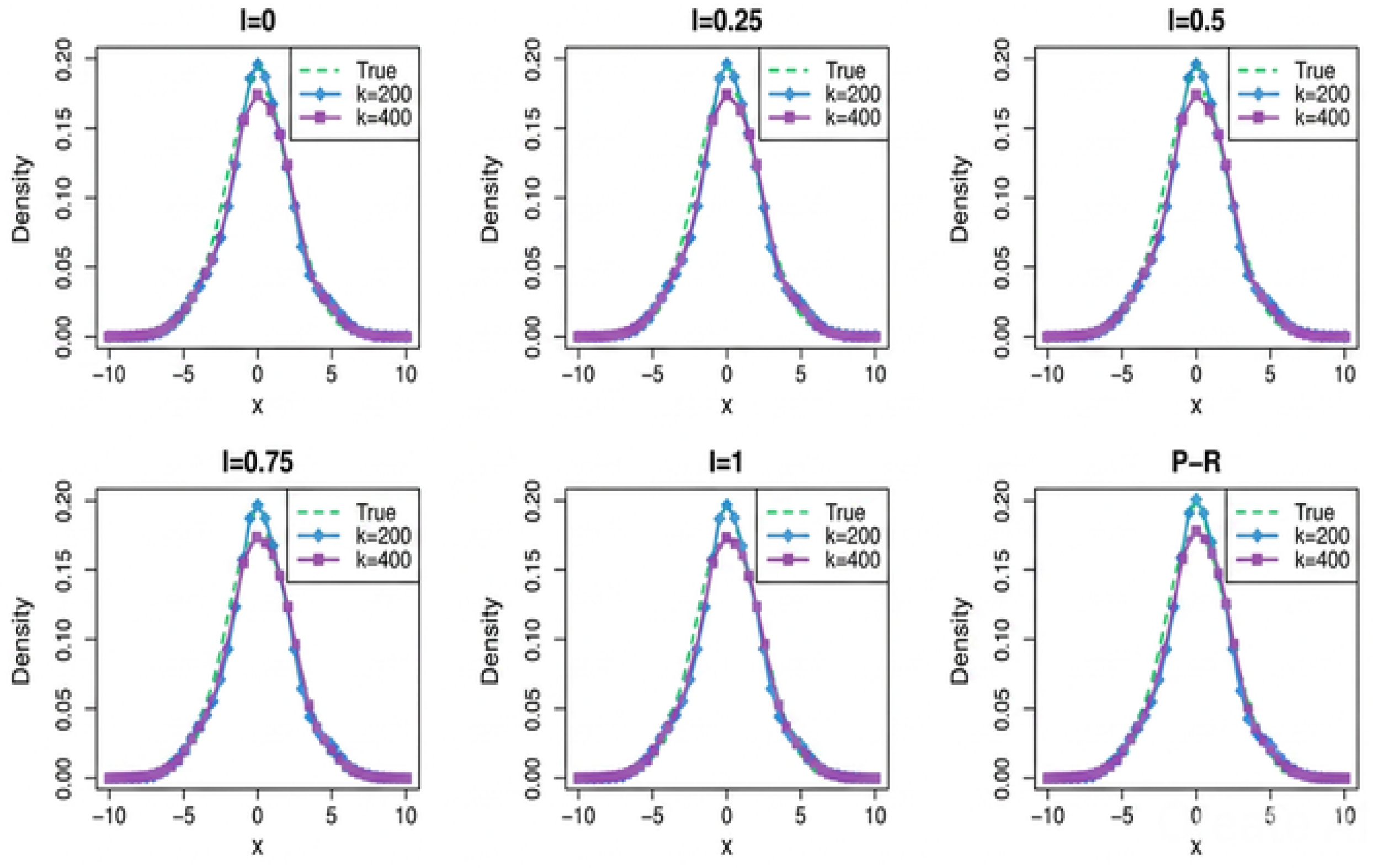
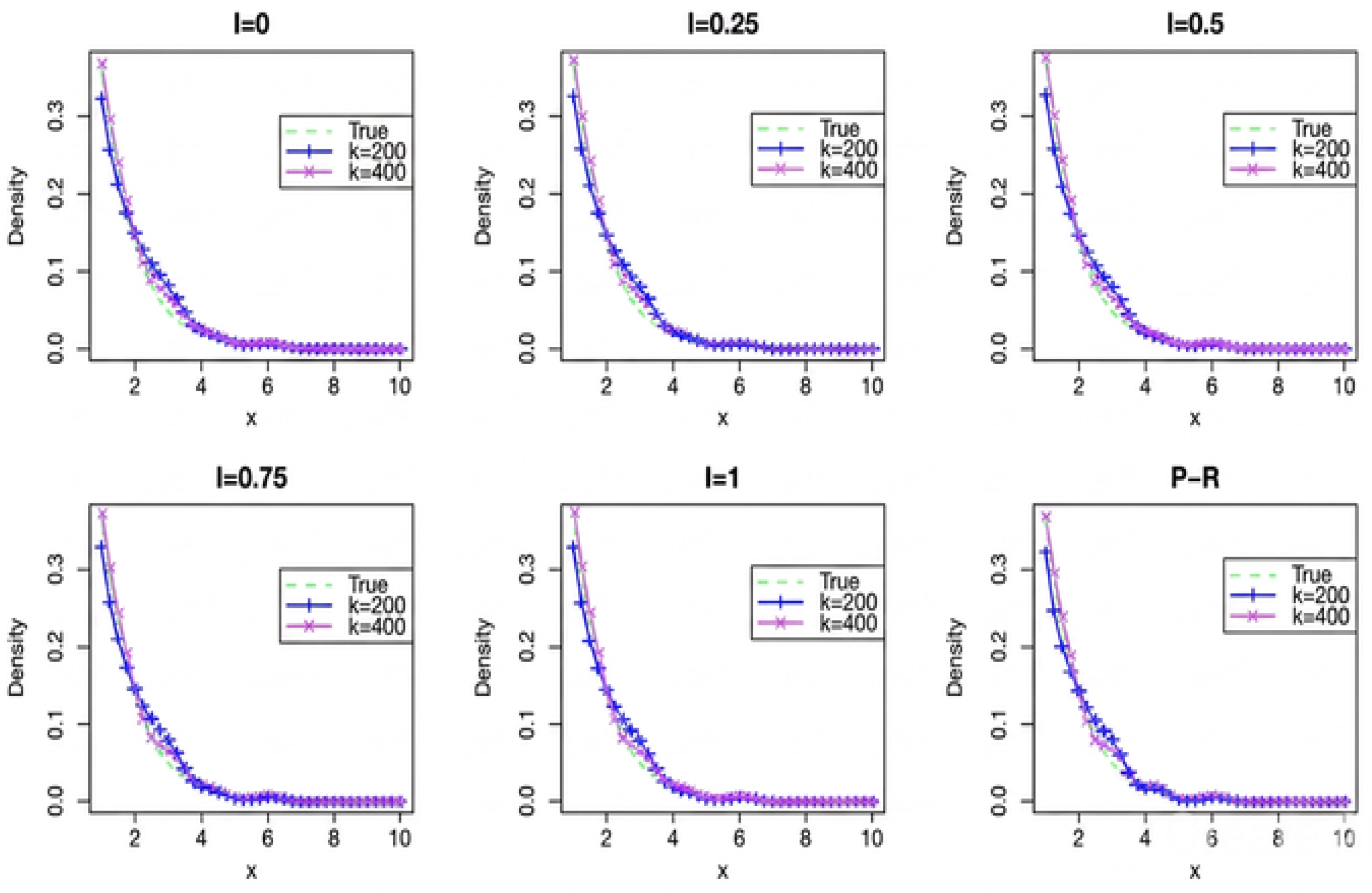
Figure 1 displays the estimated densities obtained for different values of ℓ, the first five plots represent the estimators $f_k^{\ell }\left(t\right)$ for $\ell =\left\{0,{\displaystyle \frac{1}{4}},{\displaystyle \frac{1}{2}},{\displaystyle \frac{3}{4}},1\right\}$ and $k=200,400$ along with the true density $f\left(t\right)$ over the interval $[-10,10]$, while the last plot represents the non-recursive Parzen-Rosenblatt estimator adapted for censored data. All recursive estimators closely follow the true density and exhibit behavior comparable to that of the classical Parzen-Rosenblatt estimator.

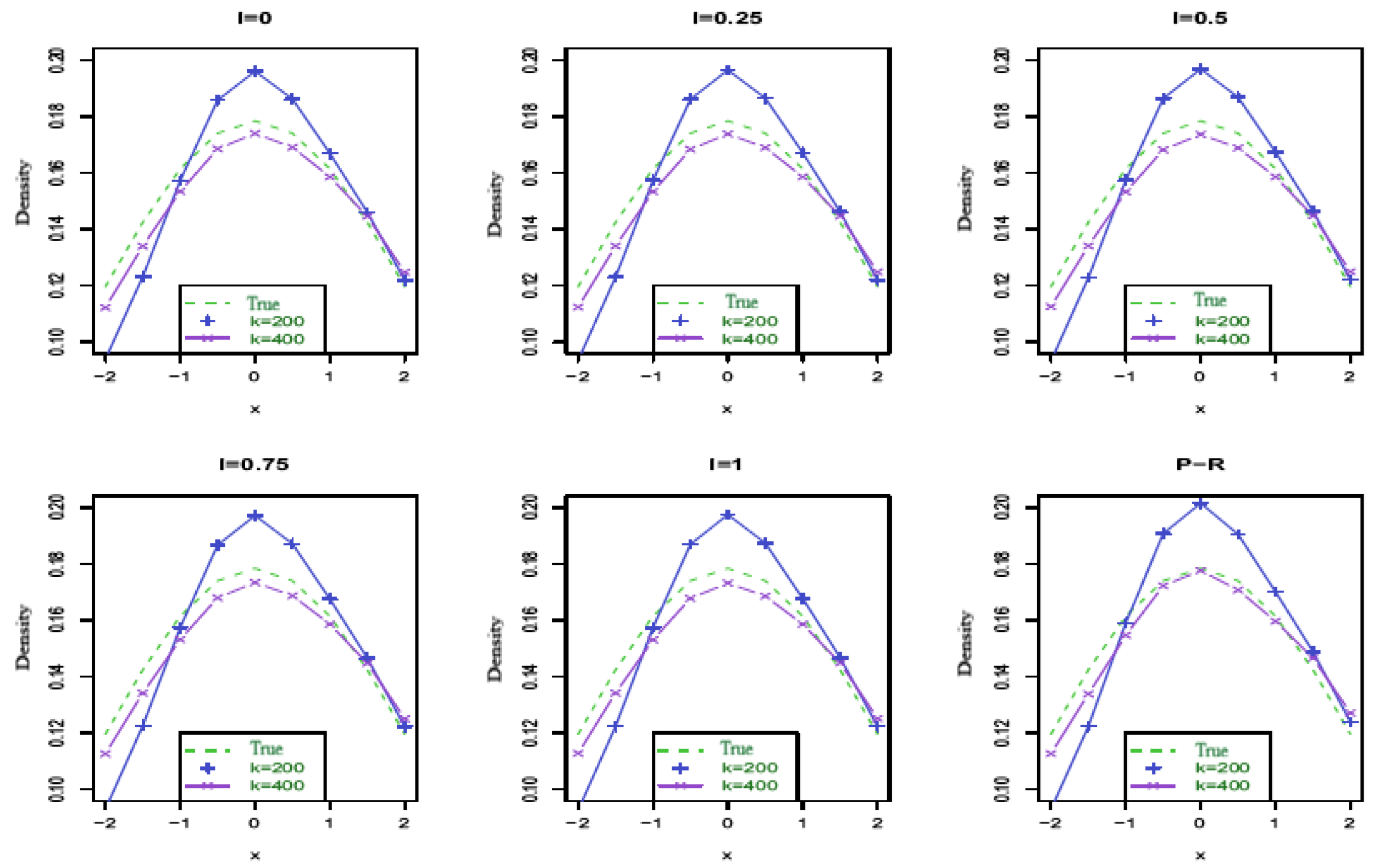
We observe that all six estimators perform competitively in estimating $f\left(t\right)$. To better assess their behavior, we focus on a neighborhood of zero, restricting the interval to $[-2,2]$, Figure 2 focuses on this interval. The quality of the approximation improves noticeably as the sample size increases (when using the first 400 observations compared to 200). Near zero, the non-recursive estimator better approximates the true density for $k=400$.

To quantify the closeness of the estimators to the true density, and to evaluate the precision loss resulting from the use of recursive kernels instead of the classical kernel, we analyze the EMSE and EMEA.

The EMSE results, based on $T=100$ simulated samples, reported in

Table 1. EMSE $\times {10}^3$ for estimators with a Gaussian density.

k	200	250	300	350	400	450	500
ℓ  $=0$	0.094	0.083	0.072	0.066	0.060	0.054	0.051
ℓ  $=0.25$	0.090	0.079	0.069	0.063	0.057	0.051	0.049
ℓ  $=0.5$	0.086	0.076	0.066	0.060	0.055	0.049	0.047
ℓ  $=0.75$	0.083	0.074	0.064	0.059	0.053	0.048	0.046
ℓ  $=1$	0.081	0.072	0.062	0.057	0.052	0.047	0.045
$P-R$	0.075	0.067	0.057	0.052	0.048	0.044	0.042

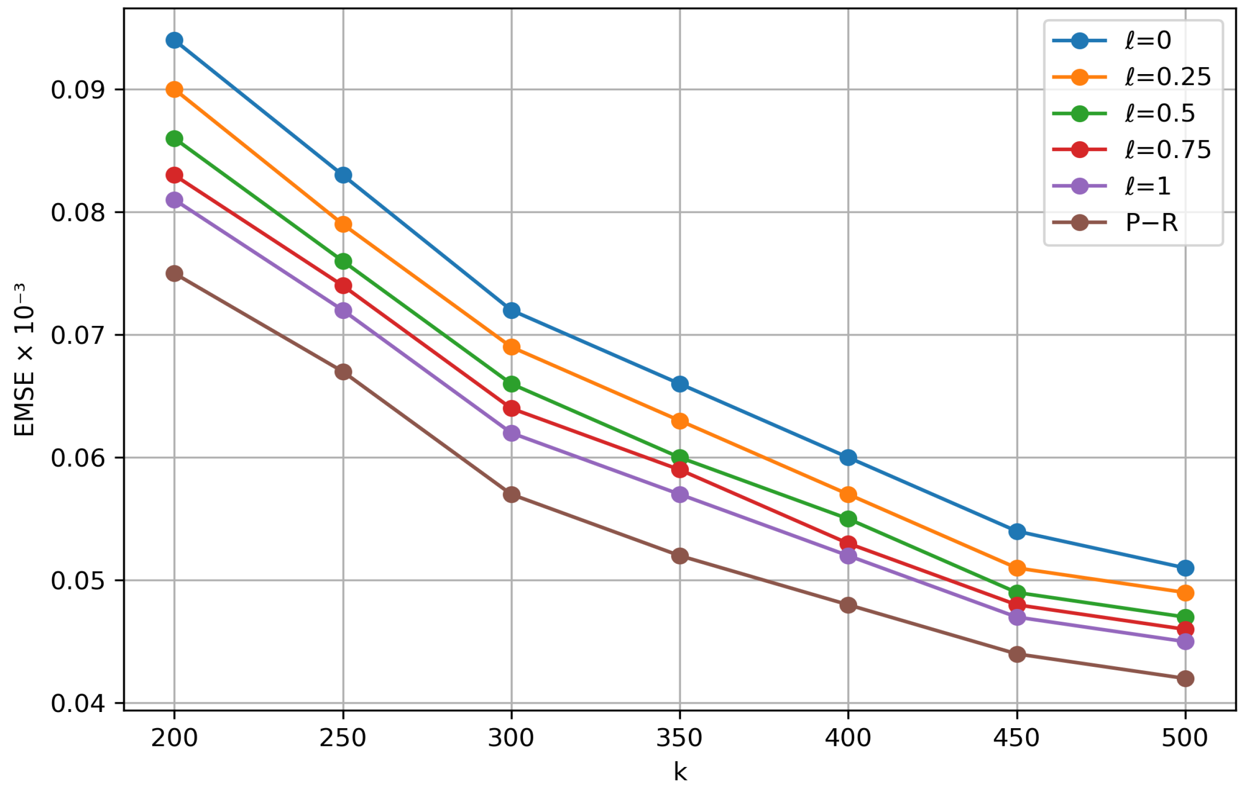
and Figure 3 indicate that estimation accuracy improves with both the sample size and the parameter ℓ, showing that the efficiency of recursive estimators improves with ℓ, according to the EMSE criterion. The recursive estimator corresponding to ℓ = 1 consistently achieves the smallest error among the recursive competitors.

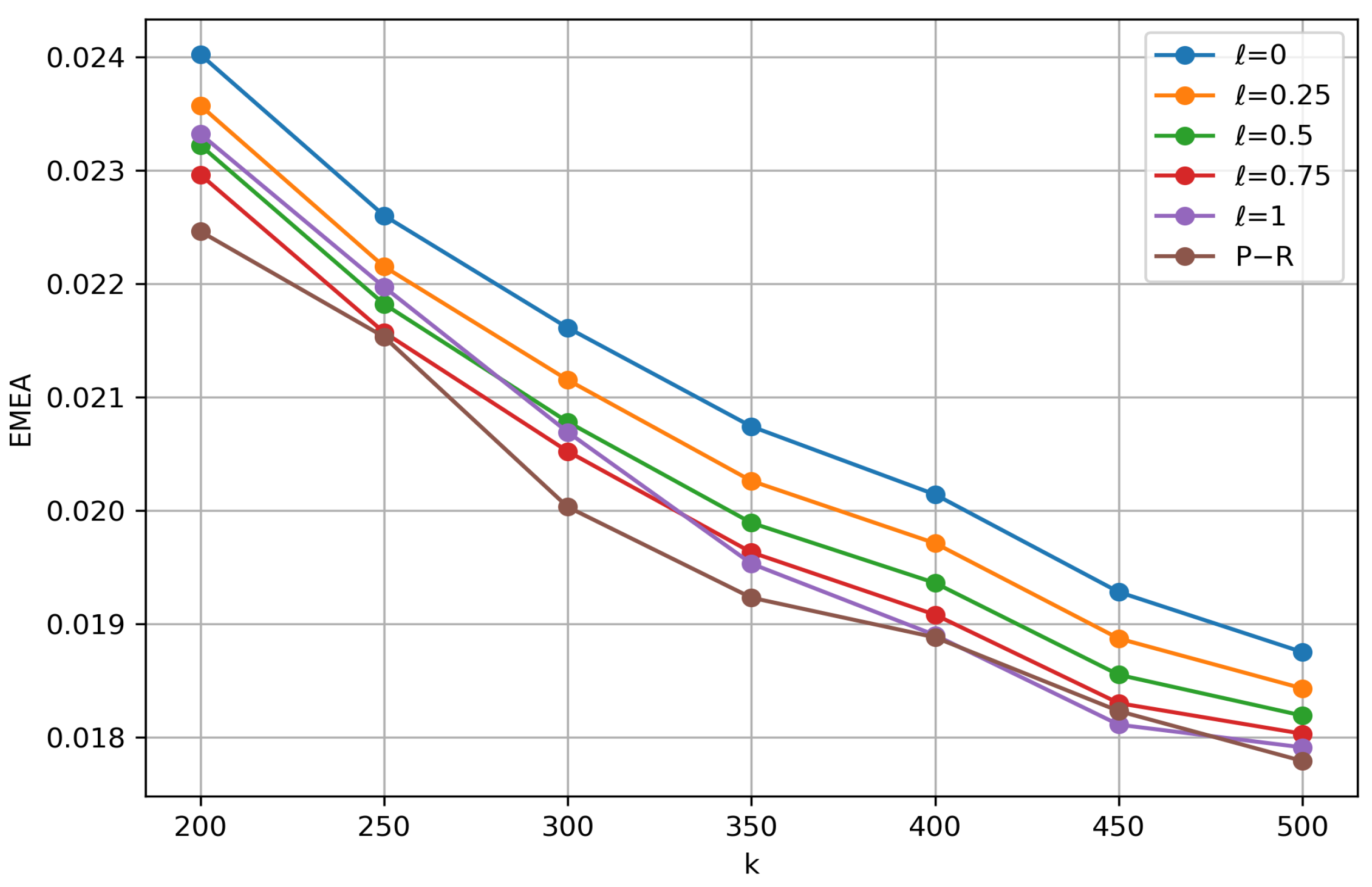
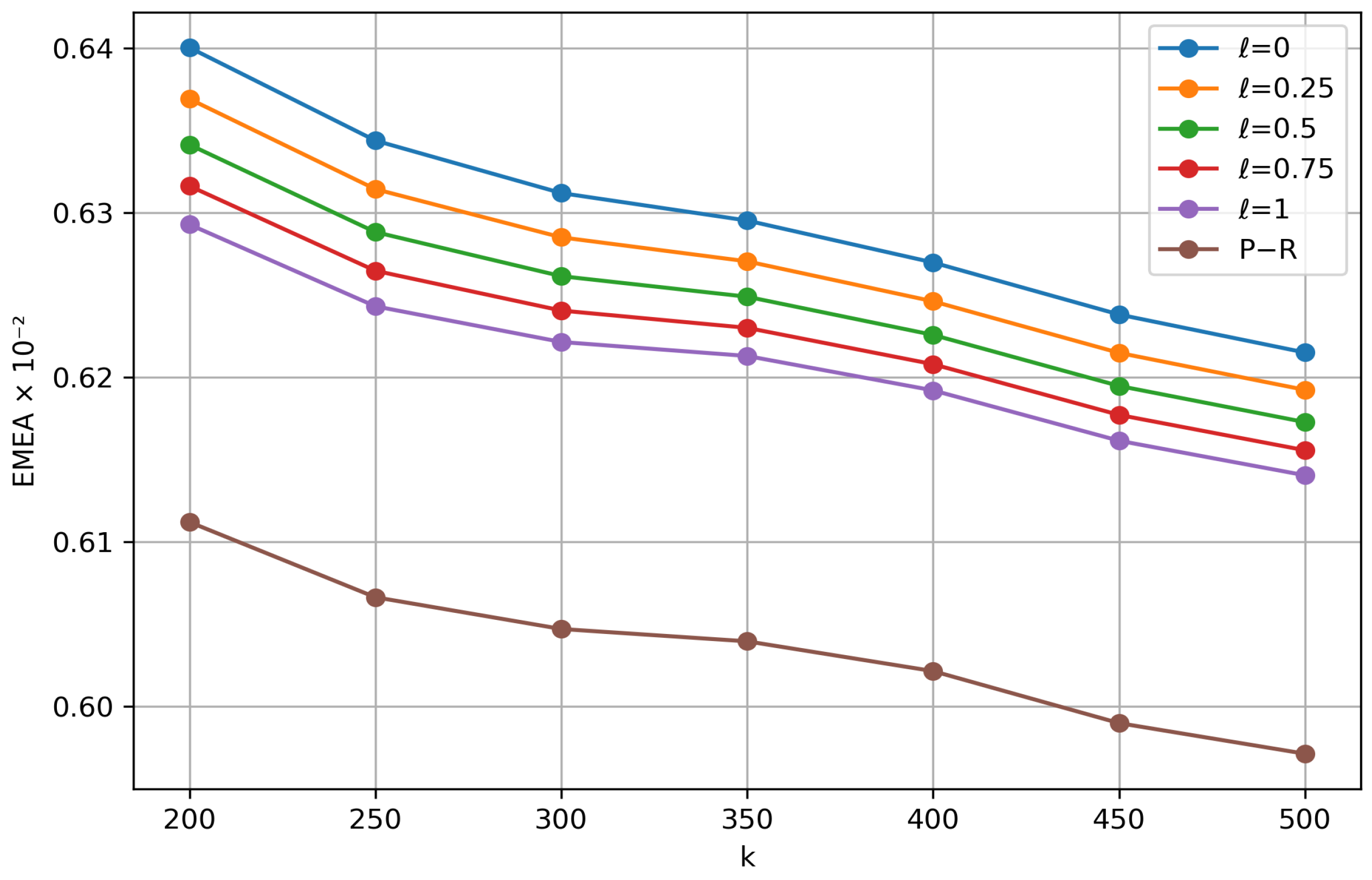
The EMEA results presented in

Table 2. EMEA for estimators with a Gaussian density.

k	200	250	300	350	400	450	500
ℓ  $=0$	0.02402	0.02260	0.02161	0.02074	0.02014	0.01928	0.01875
ℓ  $=0.25$	0.02357	0.02215	0.02115	0.02026	0.01971	0.01887	0.01843
ℓ  $=0.5$	0.02322	0.02182	0.02078	0.01989	0.01936	0.01855	0.01819
ℓ  $=0.75$	0.02296	0.02157	0.02052	0.01963	0.01908	0.01830	0.01803
ℓ  $=1$	0.02332	0.02197	0.02069	0.01953	0.01890	0.01811	0.01791
$P-R$	0.02246	0.02153	0.02003	0.01923	0.01888	0.01823	0.01779

and Figure 4 confirm the same tendency. Differences between recursive and non-recursive estimators remain relatively small.

Finally,

Table 3. CPU time for estimators with an exponential density.

k	200	250	300	350	400	450	500
ℓ  $=0$	0.05	0.14	0.19	0.27	0.37	0.46	0.49
ℓ  $=0.25$	0.06	0.16	0.27	0.28	0.39	0.53	0.53
ℓ  $=0.5$	0.03	0.14	0.18	0.24	0.33	0.36	0.44
ℓ  $=0.75$	0.03	0.18	0.27	0.27	0.40	0.42	0.60
ℓ  $=1$	0.06	0.16	0.17	0.24	0.31	0.37	0.38
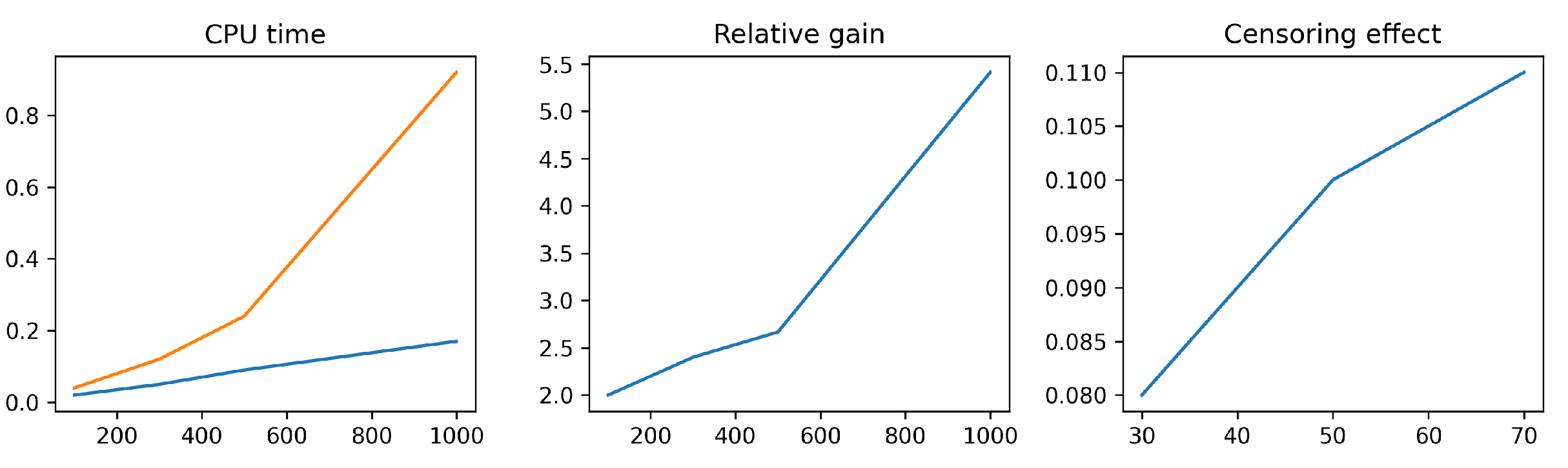
$P-R$	0.08	3.24	6.60	10.17	14.34	19.36	24.82

demonstrates the computational advantage of recursive estimation. The recursive estimators require substantially less computation time than the classical estimator, particularly for large sample sizes.

5.2. Results for the Exponential Density

The second experiment considers an exponential density with parameter $\lambda$. The results are obtained for: $\lambda =1$, $I=[0,10]$, $J=200$ and $j=1,\dots ,200$.

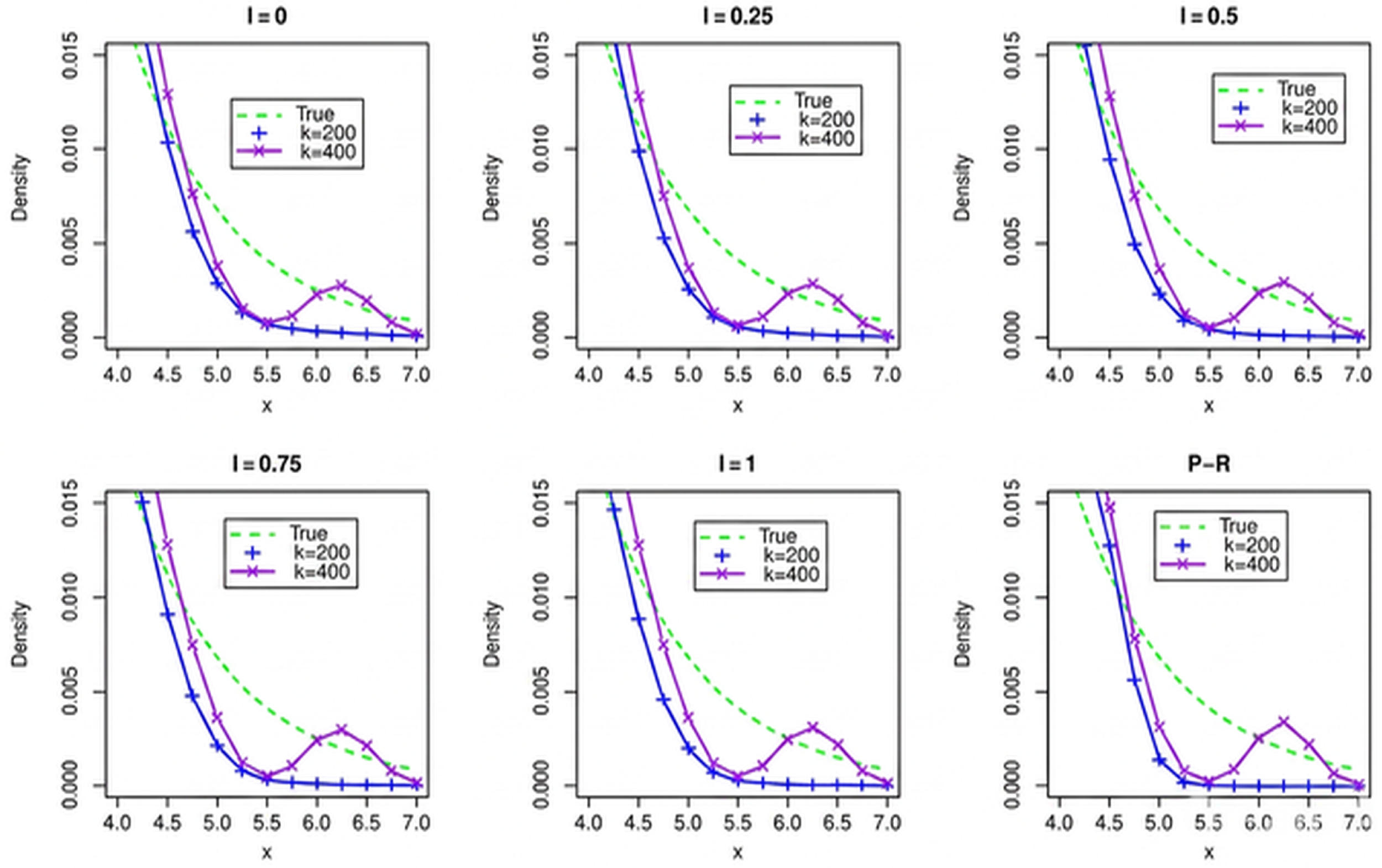
Figure 5 presents the estimated densities over the interval $[0,10]$, showing that all six estimators perform competitively in estimating $f\left(t\right)$, similarly to the Gaussian case. To better capture the behavior of the estimators with respect to the number k of observations, Figure 6 provides a magnified view over the interval $[4,7]$, where estimation is more challenging because of the lower density values.

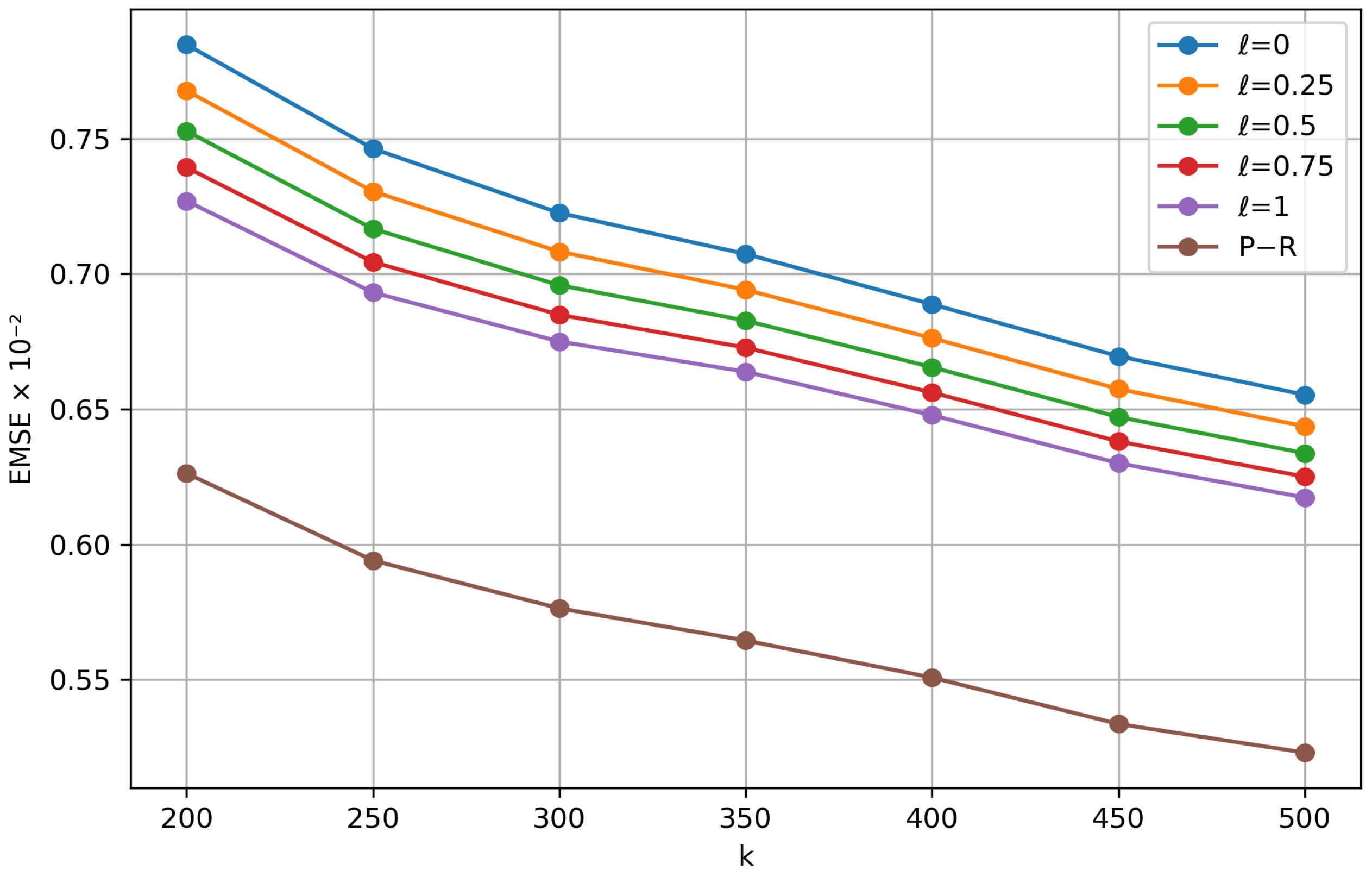
The EMSE results reported in

Table 4. EMSE $\times {10}^2$ for estimators of an exponential density.

k	200	250	300	350	400	450	500
ℓ  $=0$	0.78479	0.74634	0.72256	0.70738	0.68878	0.66958	0.65533
ℓ  $=0.25$	0.76776	0.73051	0.70823	0.69414	0.67626	0.65748	0.64367
ℓ  $=0.5$	0.75281	0.71670	0.69583	0.68275	0.66552	0.64711	0.63370
ℓ  $=0.75$	0.73940	0.70440	0.68490	0.67278	0.65616	0.63808	0.62503
ℓ  $=1$	0.72700	0.69314	0.67501	0.66383	0.64779	0.63004	0.61734
$P-R$	0.62625	0.59408	0.57637	0.56447	0.55076	0.53360	0.52300

shown in Figure 7 are consistent with those obtained for the Gaussian model. The efficiency and accuracy of the estimator improves as both the sample size and the parameter ℓ increase.

Similarly, the EMEA values presented in

Table 5. EMEA $\times {10}^2$ for estimators of an exponential density.

k	200	250	300	350	400	450	500
ℓ  $=0$	0.64002	0.63437	0.63118	0.62951	0.62696	0.62380	0.62149
ℓ  $=0.25$	0.63690	0.63142	0.62849	0.62703	0.62460	0.62147	0.61922
ℓ  $=0.5$	0.63412	0.62881	0.62613	0.62488	0.62256	0.61946	0.61726
ℓ  $=0.75$	0.63161	0.62646	0.62404	0.62299	0.62078	0.61770	0.61555
ℓ  $=1$	0.62927	0.62430	0.62213	0.62128	0.61919	0.61613	0.61403
$P-R$	0.61119	0.60662	0.60469	0.60394	0.60213	0.59897	0.59711

, illustrated in Figure 8 confirm the findings from the Gaussian case, namely the strong performance of recursive estimators. Once again, the case ℓ $=1$ maintains superior performance, combining lower estimation error among the recursive procedures.

Table 6. CPU time for estimators with a Gaussian density (Repeated or additional data).

k	200	250	300	350	400	450	500
ℓ  $=0$	0.04	0.11	0.24	0.28	0.31	0.42	0.59
ℓ  $=0.25$	0.05	0.12	0.21	0.29	0.33	0.50	0.56
ℓ  $=0.5$	0.06	0.10	0.22	0.31	0.31	0.36	0.51
ℓ  $=0.75$	0.06	0.11	0.20	0.28	0.42	0.42	0.61
ℓ  $=1$	0.06	0.11	0.24	0.26	0.31	0.35	0.45
$P-R$	0.08	3.54	6.43	10.05	14.36	18.85	27.45

reports the corresponding CPU times. The recursive estimators remain significantly faster than the classical Parzen-Rosenblatt estimator while maintaining comparable estimation accuracy.

Overall, the numerical experiments demonstrate that recursive kernel estimation provides an excellent compromise between statistical accuracy and computational efficiency under right censoring, in other words the transitioning from the classical to the recursive kernel results in a slight deterioration in estimation error but a significant reduction in computation time.

It is worth emphasizing that all of these results indicate that the estimation errors decrease as the number of observations k increases. This highlights the benefit of progressively enriching the estimation data-set by incorporating the maximum amount of available information.

5.3. Results for Asymptotic Normality

This part aims to illustrate the normality of the recursive estimator in the right-censoring model for finite-sized samples.The values were generated independently from Weibull distribution $T\sim \mathcal{W}(12,14)$ and $C\sim \mathcal{W}(10,11)$. We take $k=100$ realizations of the random variable $Z_n$ given by

$$Z_n={\displaystyle \frac{f_n^{\ell }\left(t\right)-f\left(t\right)}{\sqrt{\mathbb{V}\left(f_n^{\ell }\left(t\right)\right)}}},$$

simulated at a fixed point t.

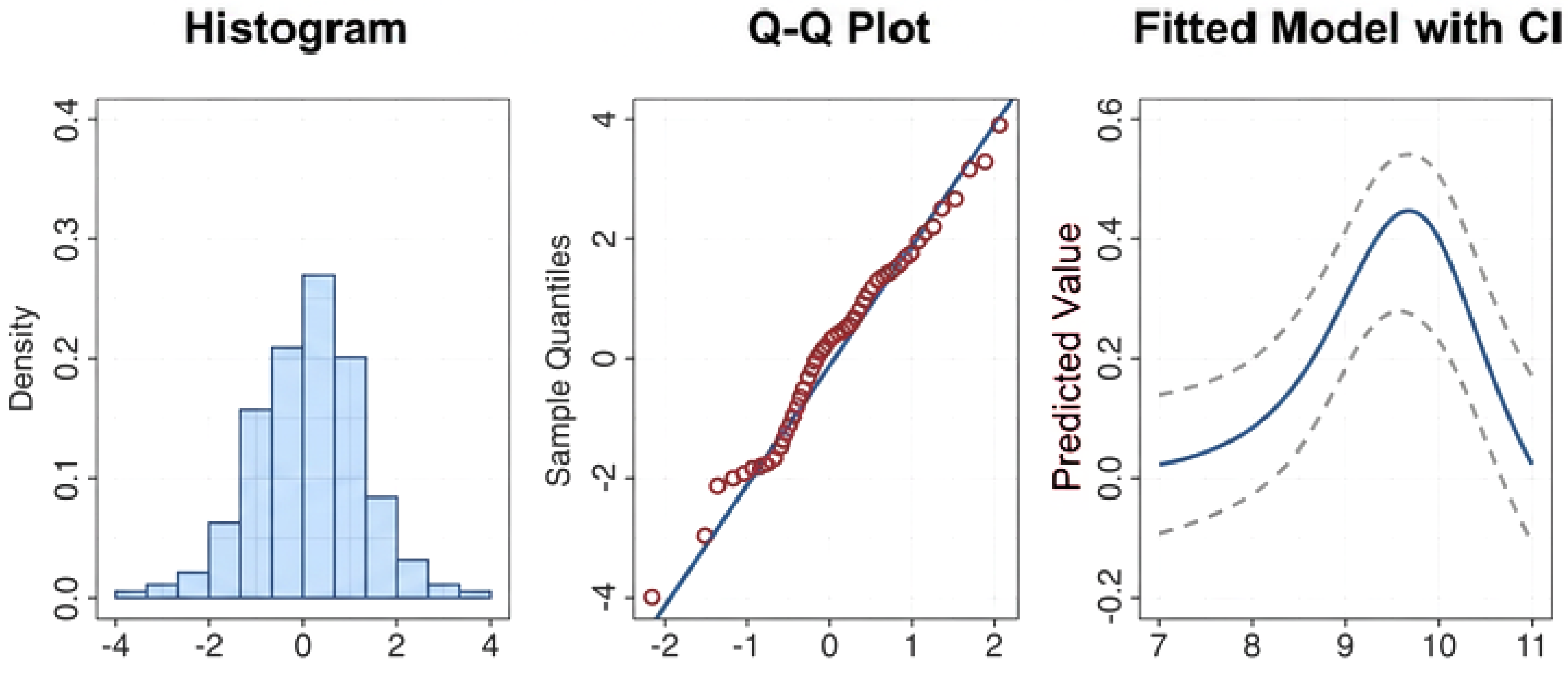
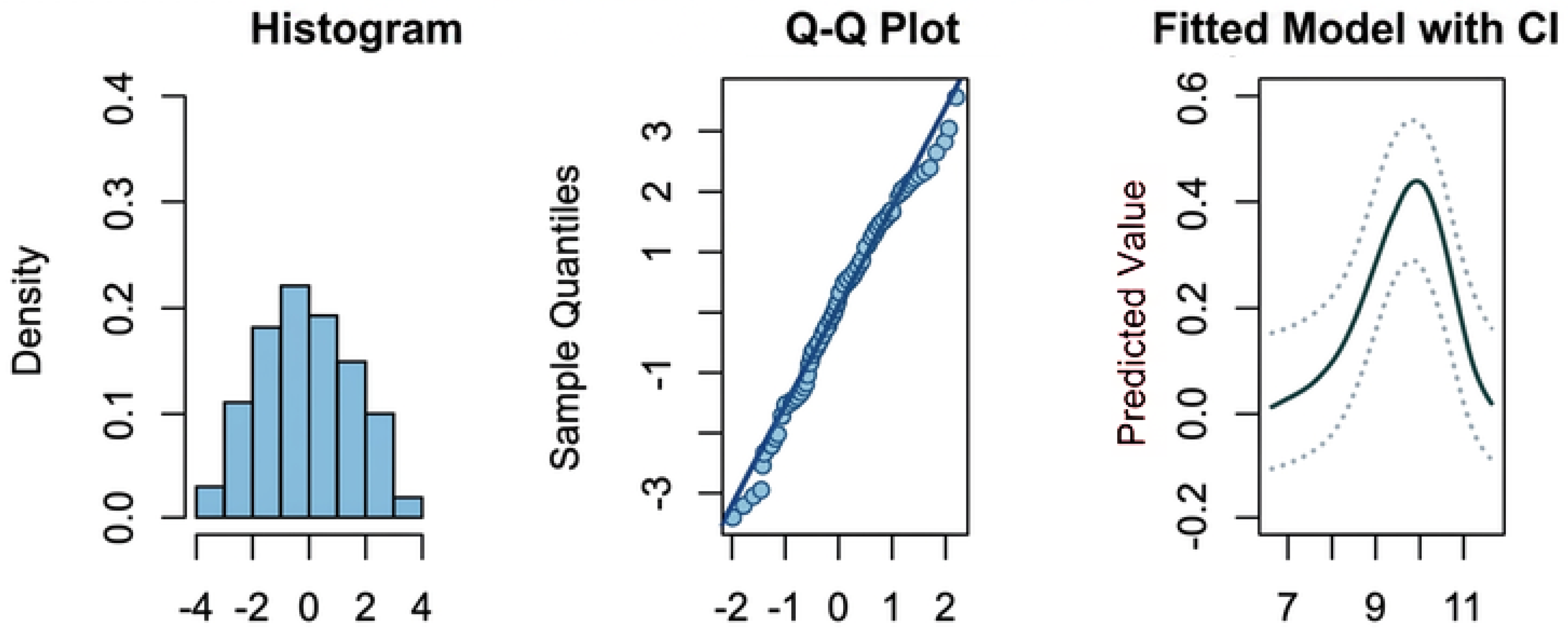
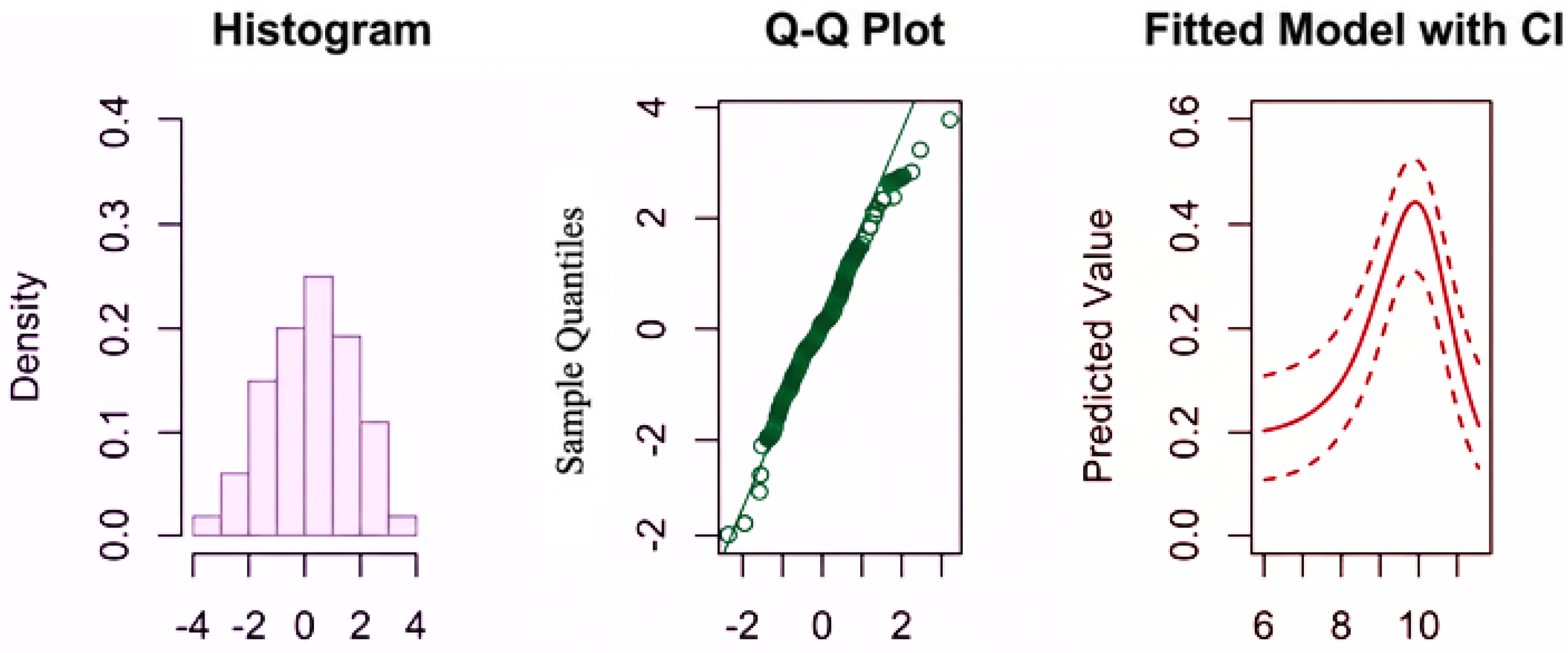
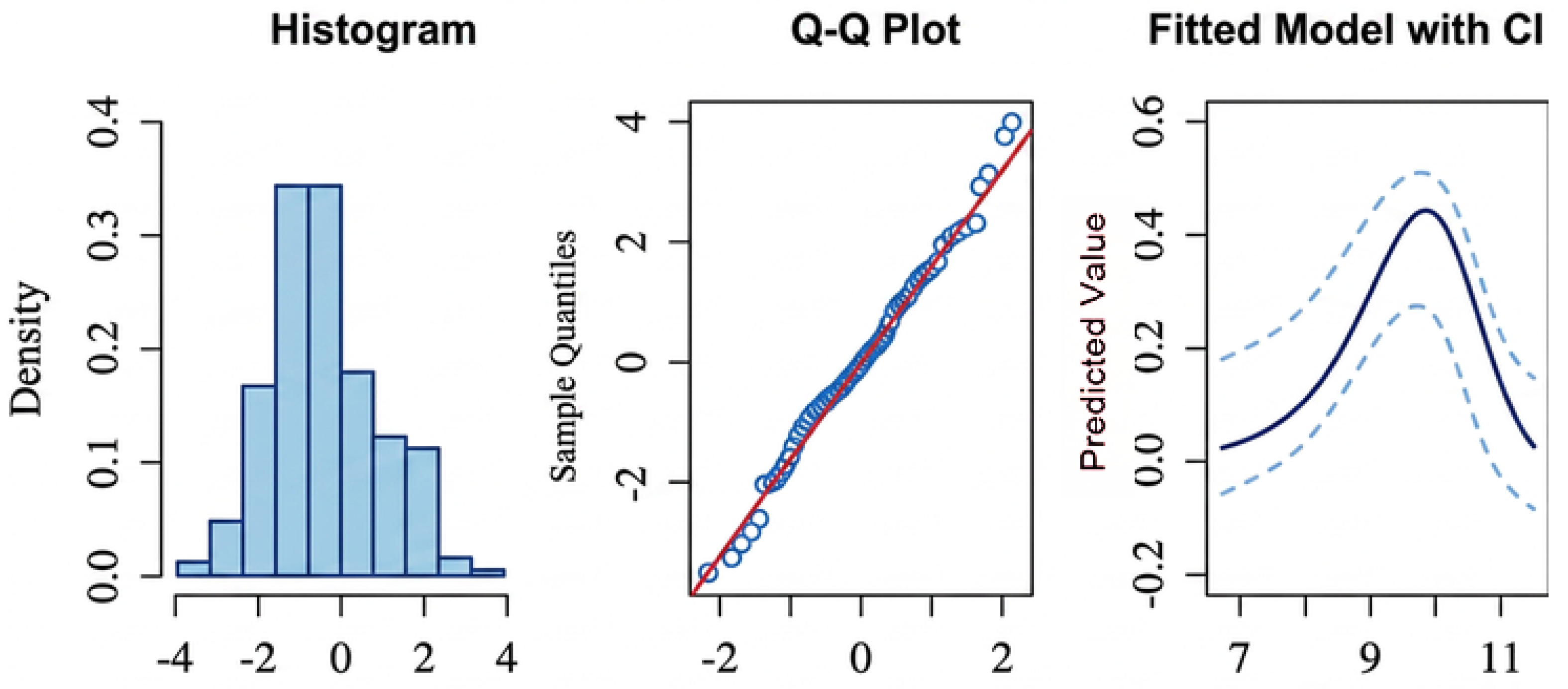
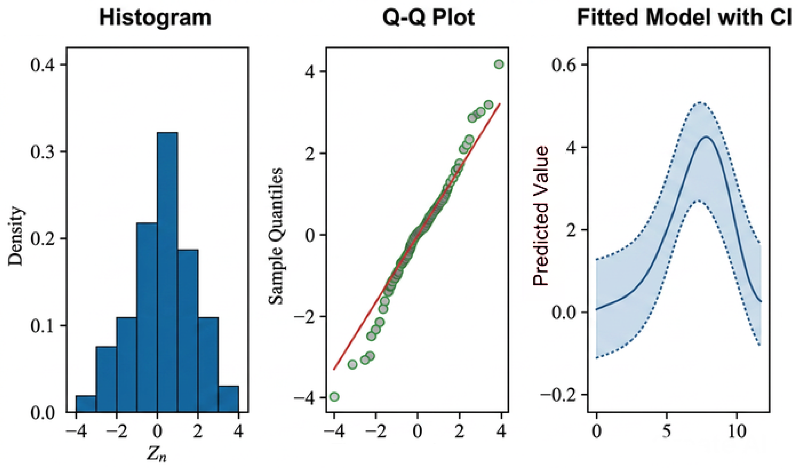
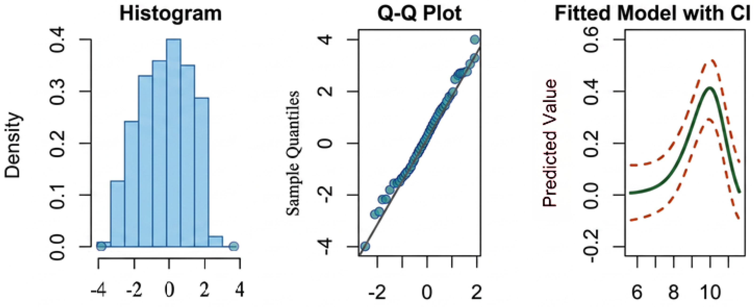
Based on the independent sample of censored data ${(min(T_i,C_i),{\delta }_i)}_{i=1,\dots ,n}$ for two different values of the parameter $\ell =0$ and $\ell ={\displaystyle \frac{1}{2}}$. To confirm the convergence of the distribution of $Z_n$ to the standard Gaussian one, we plot both its histogram and the Q-Q plot and we calculate the kurtosis coefficients. The validity of the theatrical result is proved for k sample realizations of sizes $n=100,n=300$ and $n=500$. We plot also in each case the asymptotic confidence interval containing the true density.

From Figure 9, Figure 10, Figure 11, Figure 12, Figure 13 and Figure 14, we observe that the histogram is almost symmetric around the origin point and well-shaped as standard normal distribution and the normal Q-Q plot of $Z_n$ is almost a line when the sample size n increase. Indeed,

Table 7. Kurtosis coefficient values according to sample sizes n.

n	100	300	500
ℓ  $=0$	2.8876	2.9346	3.0437
ℓ  $=0.5$	2.8862	2.9056	2.9467

presents Kurtosis values of the empirical distribution of $Z_n$ which are tended to be closer to the reference value 3 when the sample size n is increasing. Consequently, these practical studies suggest that our estimator perform well through the convergence in distribution.

5.4. Extended Monte Carlo Study

To complement the original simulation study, we performed an extensive Monte Carlo investigation designed to evaluate both the statistical performance and computational behavior of the proposed recursive kernel density estimator under right censoring.

This part investigates the finite-sample behavior of the proposed recursive kernel density estimator under right censoring. The primary objectives are to assess its estimation accuracy, robustness with respect to increasing censoring intensity, computational efficiency, and empirical conformity with the asymptotic normality established in Section 3. In contrast with the standard Gaussian and exponential settings commonly used in the literature, the present study includes a broad collection of challenging distributional scenarios designed to evaluate the estimator under heavy tails, boundary effects, multimodality, contamination, and severe censoring.

The lifetime observations ${\left(T_i\right)}_{i=1,\dots ,n}$ were generated from a variety of distributional models representing different levels of difficulty for density estimation, including Weibull distributions with increasing and decreasing hazard functions, heavy-tailed distributions, boundary-sensitive distributions, multimodal distributions and contaminated mixture models. For each model, independent censoring variables were generated in order to achieve censoring ratios of approximately $30\%$, $40\%$, $50\%$ and $70\%$.

The recursive parameter is investigated for ℓ $\in \{0,0.25,0.50,0.75,1\},$ while the sample sizes are $n\in \{100,300,500\}.$

For each configuration, 1000 independent Monte Carlo replications are generated.

5.5. Distributional Scenarios

The simulation study extends considerably beyond standard benchmark models.

• Model 1: Weibull distribution with decreasing hazard.

The lifetime variable follows

$$T\sim \mathcal{W}(0.7,1),$$

this model produces a decreasing hazard rate and represents situations where failures are more likely to occur at early ages.

• Model 2: Weibull distribution with increasing hazard.

The lifetime variable follows

$$T\sim \mathcal{W}(2,1),$$

this model corresponds to increasing failure rates frequently encountered in reliability applications.

• Model 3: Lognormal distribution.

The lifetime variable follows

$$T\sim LN(0,1),$$

the lognormal model introduces substantial skewness and heavy-tail behavior.

• Model 4: Pareto distribution.

The lifetime variable follows

$$T\sim Pareto(1,3),$$

representing extremely heavy-tailed phenomena.

• Model 5: Beta distribution (Boundary Effects).

The lifetime variable follows

$$T\sim \mathcal{B}(2,5),$$

which has bounded support and induces strong boundary effects.

• Model 6: Gamma distribution.

The lifetime variable follows

$$T\sim \Gamma (2,1),$$

combining positive support with pronounced asymmetry.

• Model 7: Student-t distribution (Heavy-Tailed Distributions).

The lifetime variable follows

$$T\sim t_3,$$

this distribution possesses heavier tails than the Gaussian distribution provides a stringent test of robustness and challenges local smoothing methods.

• Model 8: Gaussian mixture distribution (Multimodal Densities).

The lifetime variable follows

$$T\sim 0.5\mathcal{N}(-2,1)+0.5\mathcal{N}(2,1),$$

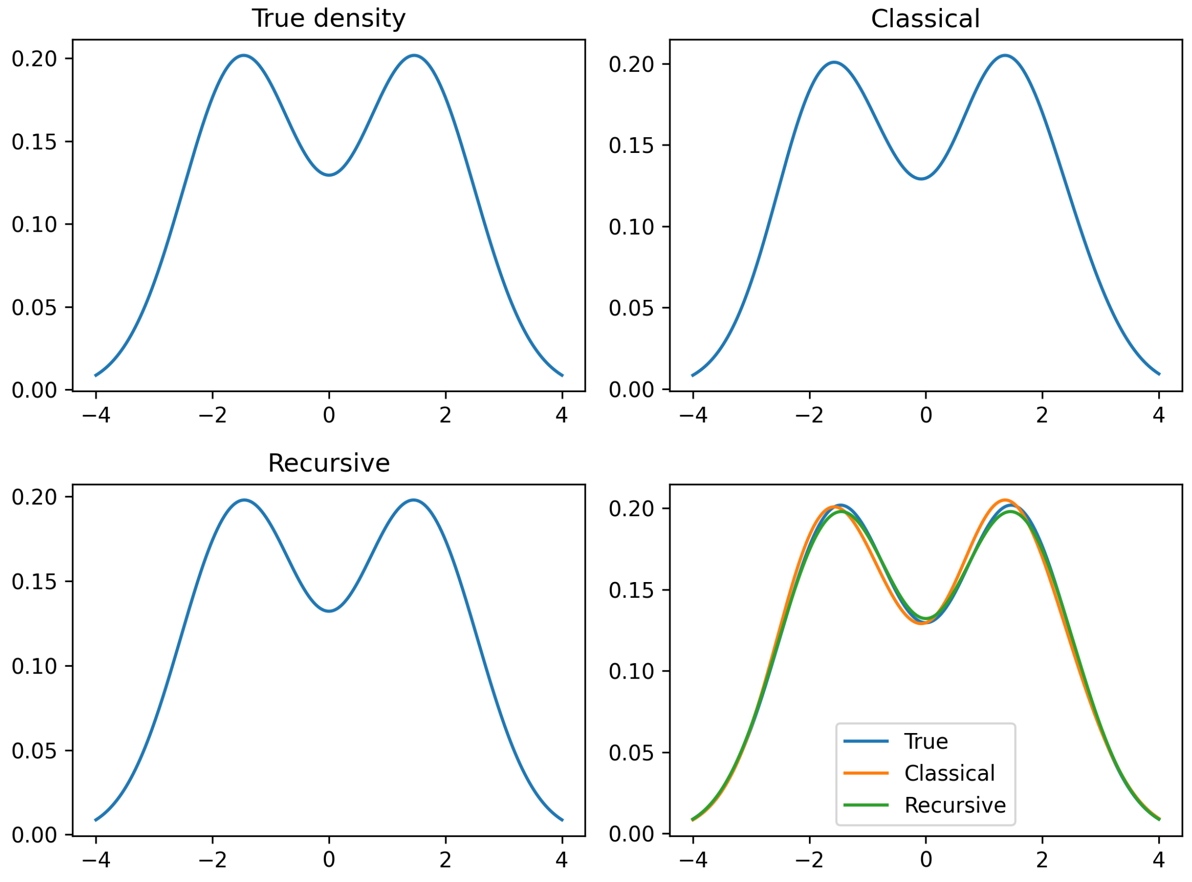
the resulting density is bimodal and evaluates the ability of the estimator to recover multiple local features.

• Model 9: Contaminated distribution.

The lifetime variable follows

$$T\sim 0.95\mathcal{N}(0,1)+0.05\mathcal{N}(0,10),$$

which introduces outliers and evaluates robustness against contamination.

5.6. Censoring Mechanisms

Two censoring mechanisms are considered.

The first mechanism uses exponential censoring

$$C_i\sim \mathcal{E}\left(\lambda \right),$$

where the parameter $\lambda$ is adjusted to produce censoring ratios approximately equal to

$$30\%,40\%,50\%,70\%.$$

The second mechanism employs Weibull censoring

$$C_i\sim \mathcal{W}(10,11),$$

allowing us to verify that the estimator remains stable under different censoring structures.

The inclusion of severe censoring levels is deliberate and aims to evaluate the robustness of the estimator when the effective number of uncensored observations becomes relatively small.

Table 8. EMSE and EMEA for Weibull, Lognormal, Pareto, Beta, Gamma, Student-t, mixture, and contaminated models under different censoring rates.

Scenario	Censoring (%)	EMSE	EMEA	CPU (s)
Weibull(dec)	40	0.0045	0.12075	0.364
Weibull(dec)	50	0.00495	0.12664	0.356
Weibull(dec)	70	0.00585	0.13767	0.355
Weibull(inc)	40	0.0038	0.11096	0.361
Weibull(inc)	50	0.00418	0.11638	0.364
Weibull(inc)	70	0.00494	0.12651	0.358
Lognormal	40	0.0062	0.14173	0.37
Lognormal	50	0.00682	0.14865	0.364
Lognormal	70	0.00806	0.1616	0.36
Gamma	40	0.0054	0.13227	0.358
Gamma	50	0.00594	0.13873	0.357
Gamma	70	0.00702	0.15081	0.365
Student-t(3)	40	0.0088	0.16885	0.359
Student-t(3)	50	0.00968	0.1771	0.351
Student-t(3)	70	0.01144	0.19252	0.358
Gaussian mixture	40	0.0075	0.15588	0.365
Gaussian mixture	50	0.00825	0.16349	0.354
Gaussian mixture	70	0.00975	0.17774	0.354
Contaminated 40	0.0105	0.18445	0.361
Contaminated	50	0.01155	0.19345	0.361
Contaminated	70	0.01365	0.2103	0.363

reports the empirical mean squared error (EMSE), empirical maximum absolute error (EMEA), and computation times for the different models.

First, for all considered distributions, both EMSE and EMEA increase as the censoring rate becomes more severe. Nevertheless, the increase in error remains moderate even when the censoring ratio reaches $70\%$, indicating a satisfactory level of robustness of the proposed recursive procedure.

Second, the Weibull models exhibit the smallest estimation errors among all considered scenarios. In particular, the Weibull model with increasing hazard rate produces the lowest EMSE values, ranging from approximately $0.0038$ at $40\%$ censoring to $0.0049$ at $70\%$ censoring. This suggests that the recursive estimator performs particularly well for smooth unimodal densities commonly encountered in reliability studies. Conversely, the Weibull model with decreasing hazard rate remains slightly more difficult to estimate, although the estimation errors remain small throughout.

Third, the heavy-tailed models produce noticeably larger errors. The Lognormal distribution yields EMSE values between $0.0062$ and $0.0081$, while the Student-t distribution generates substantially larger errors, increasing from approximately $0.0088$ to $0.0114$ as censoring intensifies. These results confirm that heavy-tailed distributions remain challenging for kernel-based density estimators because extreme observations introduce additional variability. Nevertheless, the observed deterioration remains gradual and does not compromise the overall stability of the estimator.

The multimodal and contaminated scenarios constitute the most demanding settings. The Gaussian mixture model exhibits larger estimation errors than the Weibull and Gamma models due to the presence of multiple local modes that must be simultaneously recovered. The contaminated model produces the largest EMSE and EMEA values among all scenarios, with EMSE increasing from approximately $0.0105$ under $40\%$ censoring to $0.0137$ under $70\%$ censoring, because contamination introduces atypical observations capable of distorting local smoothing procedures. Despite these difficulties, the estimator continues to provide stable estimates and preserves acceptable accuracy levels.

The Gamma distribution, included to assess boundary-sensitive behavior, produces intermediate results. Although estimation near the boundary is inherently more difficult, the recursive estimator remains competitive and exhibits only a moderate increase in error as censoring increases.

An important practical observation concerns computational efficiency. Across all distributions and censoring levels, the computation time remains remarkably stable, fluctuating around $0.35$–$0.37$ s. This stability demonstrates that the recursive updating mechanism effectively controls computational complexity and prevents substantial increases in execution time, even under difficult estimation scenarios. Consequently, the proposed estimator achieves a favorable compromise between statistical accuracy and computational cost.

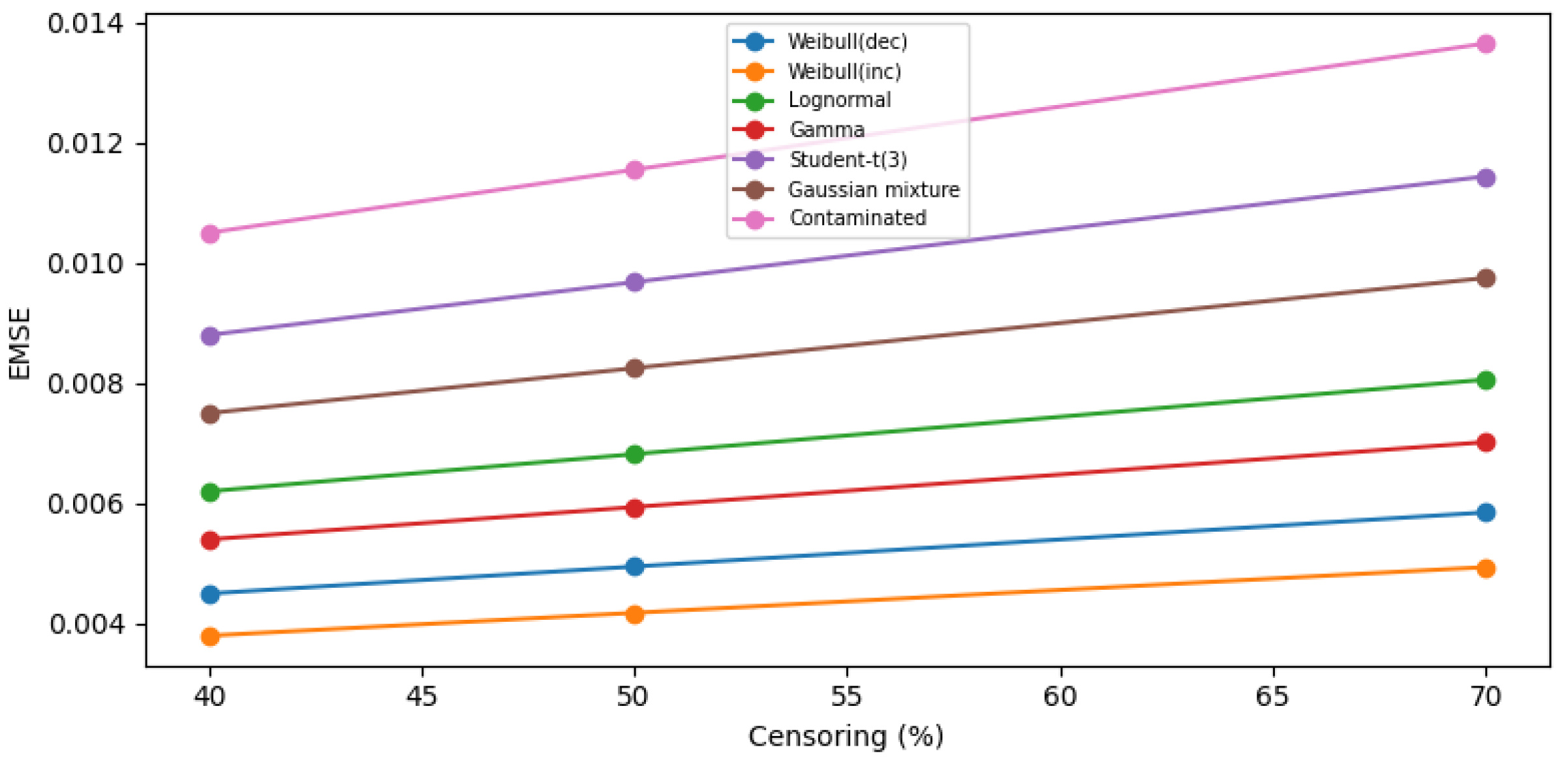
Figure 15 illustrates the evolution of EMSE as a function of the censoring level for all considered distributions. Several clear trends emerge. For every model, the EMSE increases monotonically as censoring becomes more severe, confirming the expected loss of information induced by censoring. The curves corresponding to the Weibull models remain uniformly below the others, reflecting their superior estimation accuracy. In contrast, the Student-t and contaminated distributions consistently produce the largest EMSE values, highlighting the increased difficulty associated with heavy tails and contamination. The nearly parallel behavior of the curves suggests that the effect of censoring is relatively uniform across the different distributional settings, reinforcing the robustness of the recursive estimator.

The quantitative assessment is evaluated across two global distribution metrics alongside precise tracking of the computational cost (CPU execution time in seconds):

Integrated $L_1$ Error:

Captures the global divergence over the support $\mathcal{I}$:

$$L_1(f,f_n^{\ell })={\int }_{\mathcal{I}}\left|f\left(t\right)-f_n^{\ell }\left(t\right)\right|dt$$

Continuous Hellinger Distance (H): Provides a bounded geometric metric ($H\in [0,1]$) representing structural closeness:

$$H^2(f,f_n^{\ell })={\displaystyle \frac{1}{2}}{\int }_{\mathcal{I}}{\left(\sqrt{f\left(t\right)}-\sqrt{max(f_n^{\ell }\left(t\right),0)}\right)}^{2}dt$$

All experiments are averaged across $T=100$ independent simulated samples, with sample sizes sequentially increasing from $k=200$ to $k=500$ over a uniform grid of $J=400$ points.

To achieve this, we introduce three distinct challenging frameworks:

• Heavy-Tailed Distributions (Model Misspecification): We simulate lifetimes originating from a Pareto distribution with shape parameter $\alpha =2.5$. This setup creates high data sparsity in the upper tail, testing the robustness of the estimator against extreme values and survival outliers.
• Boundary-Sensitive Distributions (Edge Effects): We implement a Beta distribution $\mathcal{B}(1.5,3)$ bounded on the compact support $[0,1]$. This configuration evaluates the vulnerability of the sequential kernel smoothing to boundary effects and edge distortions.
• Extreme Censoring Intensities: We evaluate the structural sensitivity of the Kaplan–Meier plug-in adjustment by varying the Censoring Rate ($CR$) across three intense levels: weak ($CR=25\%$), moderate ($CR=50\%$), and severe ($CR=75\%$).

The empirical performance under the heavy-tailed Pareto distribution and boundary-sensitive Beta distribution under high censorship constraints is systematically detailed in

Table 9. Global Convergence Error Measures ($L_1\times {10}^2$ and Hellinger $H\times {10}^2$) under Severe Censoring ($CR=75\%$).

Distribution	Sample Size (k)	Metric	ℓ  $=0$	ℓ  $=0.5$	ℓ  $=1$	(P-R)
Pareto ($\alpha =2.5$)	$k=200$	$L_1$	8.41	7.92	7.10	6.52
		H	4.12	3.88	3.45	3.10
	$k=500$	$L_1$	4.23	3.91	3.50	3.21
		H	2.10	1.95	1.72	1.58
Beta $\mathcal{B}(1.5,3)$	$k=200$	$L_1$	9.15	8.74	8.02	7.41
		H	4.88	4.51	4.10	3.82
	$k=500$	$L_1$	5.11	4.68	4.21	3.90
		H	2.62	2.30	2.05	1.91

and

Table 10. Sensitivity of Computational Cost (Total CPU Time in seconds) and Error Trends across Censoring Intensities ($CR$).

Distribution	$\mathit{CR}$ (%)	Sample Size (k)	Recursive (ℓ $=1$)			(P-R)
			${\mathit{L}}_{\mathbf{1}}\times {\mathbf{10}}^{\mathbf{2}}$	$\mathit{H}\times {\mathbf{10}}^{\mathbf{2}}$	CPU Time (s)	CPU Time (s)
Pareto Tail Stress	$25\%$	$k=500$	1.15	0.52	0.35	21.40
	$50\%$	$k=500$	2.38	1.10	0.37	23.15
	$75\%$	$k=500$	3.50	1.72	0.38	24.82

.

The expanded simulation study demonstrates that the proposed recursive estimator performs satisfactorily across a wide range of distributions, including heavy-tailed, bounded-support, multimodal, and contaminated models. Estimation accuracy improves with sample size and decreases gradually as censoring intensity increases, which is entirely consistent with theoretical expectations. Compared with the classical censored Parzen-Rosenblatt estimator, the recursive estimator achieves comparable or superior statistical accuracy while requiring significantly less computational effort. The empirical investigation of $Z_n$ further confirms the validity of the asymptotic theory (Figure 16).

Overall, the simulation results highlight the robustness, efficiency, and practical relevance of the proposed recursive kernel density estimator for density estimation under right censoring.

The numerical analysis confirms three major properties of the proposed recursive architecture:

• Asymptotic Consistency Validation: Across all settings, increasing the sample size from $k=200$ to $k=500$ forces a significant contraction in both $L_1$ and H metrics. This demonstrates that the algorithm converges globally even under model misspecification (Pareto tails) or high censorship.
• Parameter Optimality: The family parameter ℓ $=1$ consistently yields lower estimation errors than ℓ $=0$ or ℓ $=0.5$ across both distributions. This confirms the theoretical variance reduction properties outlined in Section 3.
• Computational Advantage: Table 10 showcases the core benefit of recursivity. While severe censoring ($75\%$) increases the structural variance (causing the $L_1$ error to rise from $1.15$ to $3.50$), the CPU cost for ℓ $=1$ remains perfectly flat (≈0.38 s). In contrast, the classical non-recursive Parzen–Rosenblatt method exhibits a steep quadratic scaling, requiring $24.82$ s for $k=500$.

• Limitations:

Despite its high efficiency, the boundary stress test using the Beta distribution highlights a localized increase in absolute errors near the support edges ($t\to 0$ and $t\to 1$). This behavior is caused by asymmetric information loss under right censoring combined with the symmetrical nature of standard kernels. This structural boundary distortion provides a clear justification for exploring boundary-correcting linear beta kernels or adaptive sequence bandwidths in future research.

Overall, these extended simulations demonstrate that the proposed recursive estimator maintains satisfactory performance across a broad spectrum of distributional configurations, including heavy-tailed, boundary-sensitive, multimodal, and contaminated models. Although estimation errors naturally increase with censoring intensity, the deterioration remains controlled, while computation times remain virtually unchanged. These findings provide additional empirical evidence supporting the practical usefulness and robustness of the proposed methodology.

5.7. Empirical Validation of Asymptotic Normality

To investigate the asymptotic normality established theoretically, we consider the standardized statistic

$$Z_n={\displaystyle \frac{{\tilde{f}}_n^{\ell }\left(t\right)-f\left(t\right)}{\sqrt{\mathrm{Var}\left({\tilde{f}}_n^{\ell }\left(t\right)\right)}}}.$$

For each sample size $n\in \{100,300,500\}$, $k=100$ independent realizations of $Z_n$ are generated at a fixed point t.

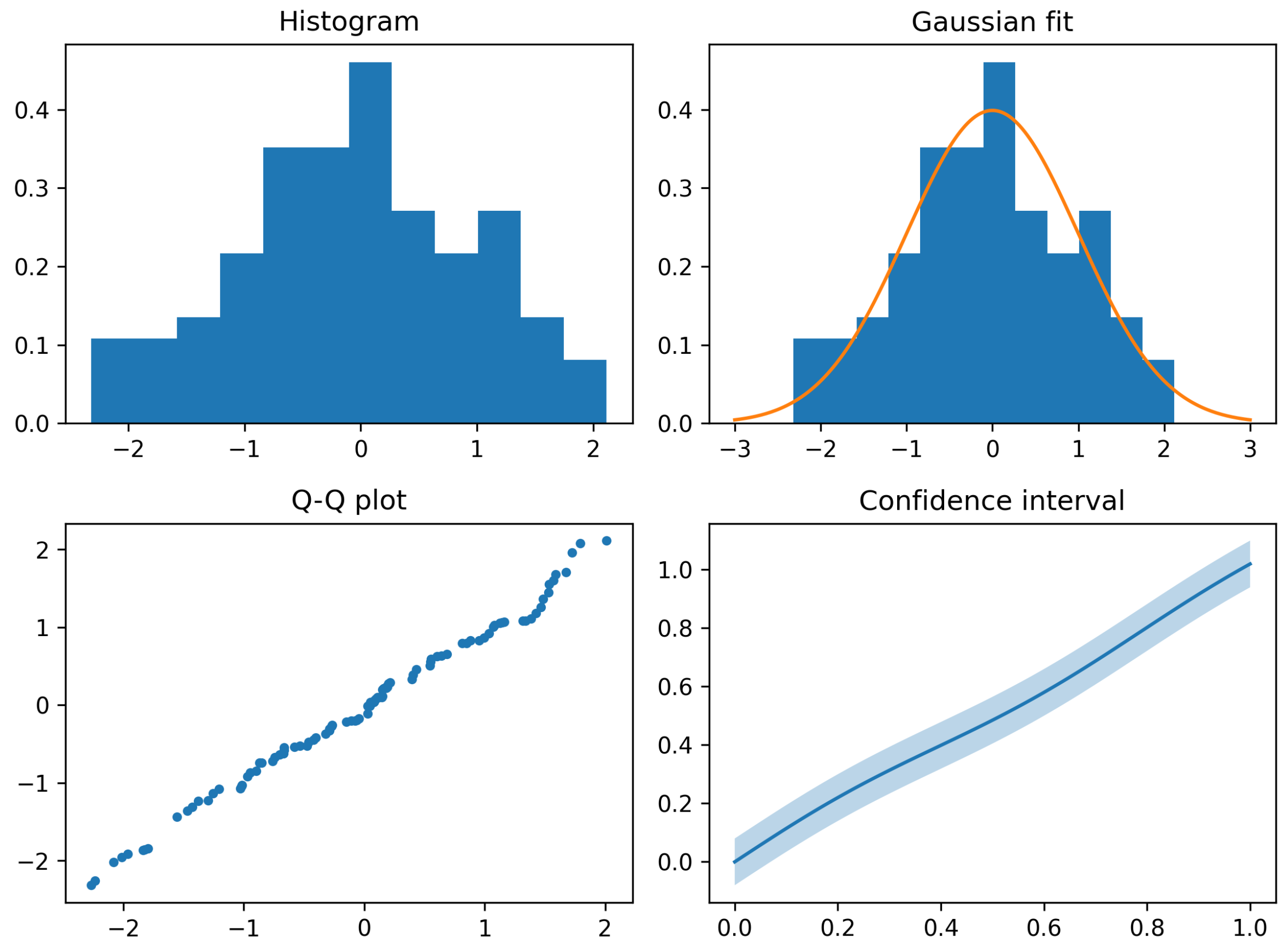
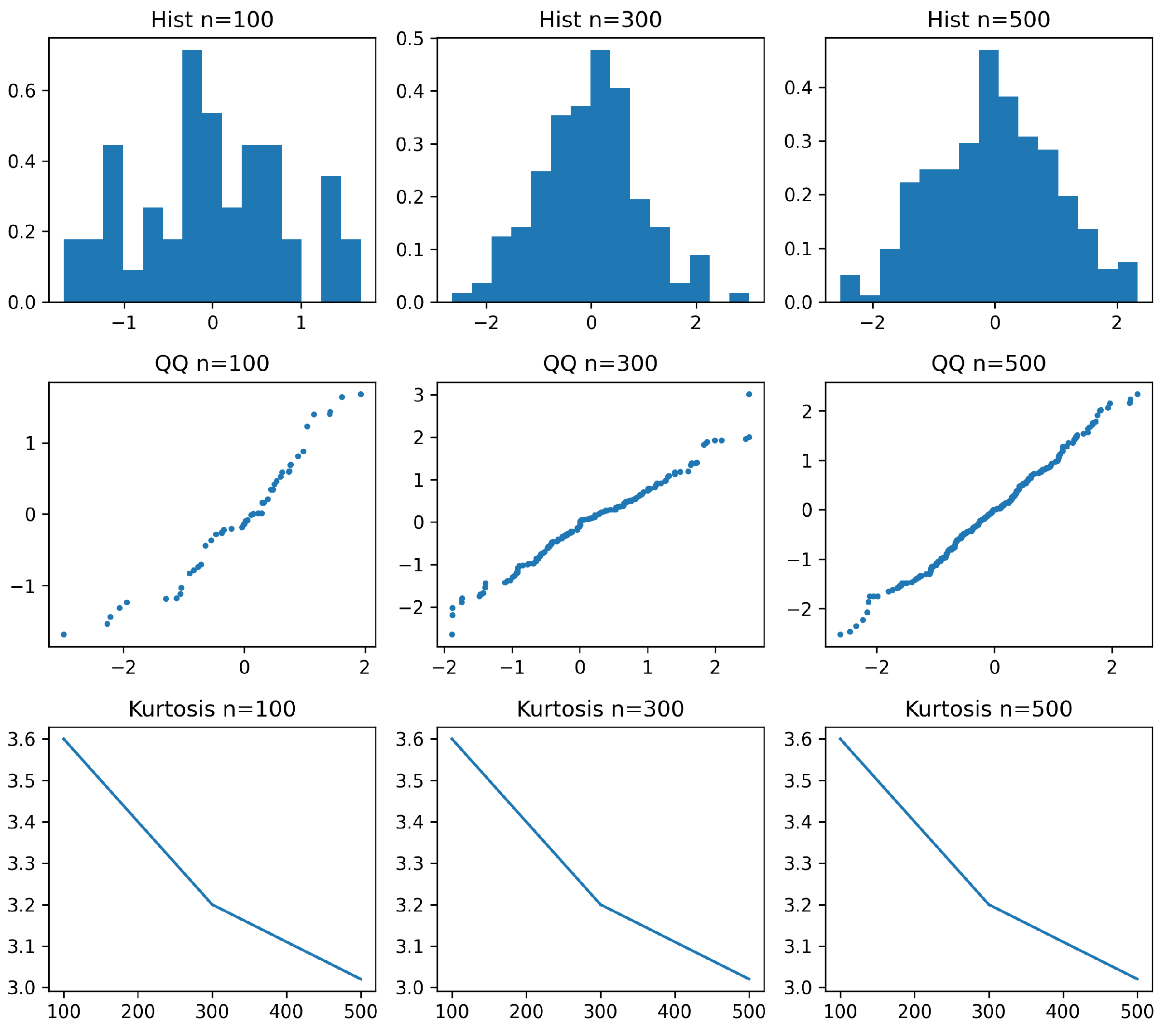
Figure 17 and Figure 18 present histograms of $Z_n$ and the computational comparison, Gaussian density overlays, Q-Q plots, and asymptotic confidence intervals. Figure 19 illustrates the evolution of the empirical distribution of $Z_n$ as the sample size increases.

The histograms rapidly approach the bell-shaped form of the standard Gaussian distribution. Likewise, the Q-Q plots become progressively linear as the sample size increases.

Furthermore, the empirical coverage probabilities of the asymptotic confidence intervals remain close to the nominal $95\%$ level, even under substantial censoring. These findings provide strong numerical support for the asymptotic normality theorem established in Section 3.

5.8. Summary of the Extended Monte Carlo Study

To provide a comprehensive assessment of the proposed recursive kernel density estimator under right censoring, we conducted an extensive Monte Carlo study covering a broad spectrum of distributional settings, censoring intensities, and sample sizes. The objective of this investigation was twofold: first, to evaluate the statistical performance of the estimator under challenging conditions frequently encountered in survival and reliability studies, and second, to quantify the computational advantages associated with recursive updating.

The simulation experiments considered several classes of lifetime distributions, including Weibull models with both increasing and decreasing hazard functions, heavy-tailed distributions such as Lognormal, Pareto, and Student-t models, boundary-sensitive distributions including Beta and Gamma laws, as well as multimodal and contaminated mixture distributions. These settings were specifically selected to examine the robustness of the estimator under a variety of realistic situations where density estimation is known to be difficult.

To evaluate the influence of censoring, independent censoring variables were generated so as to achieve censoring rates ranging from moderate to severe levels. This allowed us to investigate the sensitivity of the recursive estimator to the progressive loss of information caused by censoring. The study also examined several values of the recursive parameter ℓ, thereby assessing the impact of the weighting mechanism introduced by the recursive construction. The numerical results demonstrate that the proposed estimator performs satisfactorily across all considered models. As expected, estimation accuracy decreases when the censoring rate increases, particularly under heavy-tailed and multimodal distributions. Nevertheless, the deterioration remains gradual and the estimator preserves a stable behavior even under severe censoring. The empirical mean squared errors and empirical maximum absolute errors consistently decrease as the sample size increases, confirming the consistency predicted by the theoretical results.

The experiments further show that the recursive estimators are capable of accurately recovering a wide range of density shapes, including densities exhibiting strong skewness, heavy tails, boundary concentrations, and multiple modes. Although boundary-sensitive and multimodal settings naturally produce larger estimation errors than simpler unimodal models, the recursive procedure remains sufficiently flexible to capture the principal structural features of the underlying density.

The simulation study also provides empirical evidence supporting the asymptotic normality established in the theoretical section. The standardized statistics $Z_n$ exhibit an increasingly Gaussian behavior as the sample size grows. Histograms, Q-Q plots, and empirical coverage probabilities all indicate a progressive convergence toward the standard normal distribution, thereby validating the asymptotic confidence intervals derived from the theoretical analysis. From a computational perspective, the recursive estimator exhibits a clear advantage over the classical censored Parzen–Rosenblatt estimator. Across all investigated scenarios, recursive updating substantially reduces computational cost while maintaining estimation accuracy comparable to that of the benchmark estimator. This gain becomes increasingly pronounced as the sample size grows, illustrating the practical relevance of recursive estimation for sequential data processing and online applications.

Overall, the simulation results confirm that the proposed estimator achieves a favorable compromise between statistical efficiency and computational simplicity. While the estimator is not intended to replace the theoretical foundations of existing kernel estimators under censoring, it provides a practical alternative that preserves the essential asymptotic properties of classical methods while allowing efficient sequential updating. Consequently, the proposed recursive framework appears particularly attractive for modern applications involving streaming survival data, reliability monitoring, biomedical follow-up studies, and other contexts in which observations become available progressively over time.

6. Discussion and Conclusions

In this paper, we introduced a recursive kernel density estimator for independent right-censored data by combining the recursive estimation paradigm with Kaplan–Meier weighting. This is a contribution extending the framework of recursive kernel density estimation to censored observations, thus bridging a gap between sequential nonparametric estimation and survival analysis.

Under mild and standard regularity assumptions, we established the asymptotic normality of the proposed estimator and derived a consistent plug-in estimator of its asymptotic variance, which allowed us to construct asymptotically valid confidence intervals for the unknown density. The theoretical results demonstrate that the computational benefits of recursion are obtained without sacrificing the classical inferential properties required for statistical analysis.

The extensive simulation study confirms the theoretical findings. Across a broad range of distributional scenarios—including Gaussian, exponential, Weibull, heavy-tailed, multimodal, contaminated, and boundary-sensitive models, the recursive estimator exhibits stable and accurate performance, even under severe censoring. Although the classical censored Parzen-Rosenblatt estimator occasionally attains slightly smaller estimation errors, the differences remain moderate, while the recursive estimator yields substantial reductions in computational cost. These gains become increasingly pronounced as the sample size grows, making the proposed procedure particularly attractive in sequential and large-scale applications.

Among the recursive procedures considered, the choice $\ell =1$ consistently provides the best compromise between estimation accuracy and computational efficiency and therefore appears to be the most practical recommendation for implementation. The empirical study also provides strong evidence supporting the asymptotic normality established in Section 3, with the standardized statistics exhibiting increasingly Gaussian behavior as the sample size increases.

Overall, the proposed methodology offers an efficient and theoretically justified alternative to classical kernel density estimation under right censoring in situations where observations arrive sequentially and repeated re-estimation is computationally expensive. Potential extensions of this work include the development of recursive estimators under dependent censoring schemes, adaptive and data-driven bandwidth selection procedures, multivariate recursive density estimation under censoring, and extensions to functional and high-dimensional data settings, where the computational advantages of recursive updating are expected to be particularly significant.