Large Sample Theory for Some Ridge-Type Regression Estimators

Abstract

This paper provides a large sample theory for some ridge-type multiple linear regression estimators, including Liu-type regression estimators, when the number of predictors is fixed. Some large sample theory is also given for ridge-type generalized linear model estimators. The estimators can be used for inference and variable selection.

1. Introduction

There are outlier resistant and non-outlier resistant ridge-type estimators for multiple linear regression, and ridge-type regression estimators for generalized linear models. Section 2 of this paper gives large-sample theory for several of these ridge-type regression estimators, proving that the estimators are consistent and asymptotically normal. Section 3 shows how to use the estimators for inference such as confidence intervals, confidence regions, and hypothesis testing. This section reviews the multiple linear regression model, some ridge-type regression estimators, and the large-sample theory for the ordinary least squares estimator.

Suppose that the response variable $Y_i$ and at least one predictor variable $x_{i,j}$ are quantitative with $x_{i,1}\equiv 1$. Let ${\mathit{x}}_i^T=(x_{i,1},\dots ,x_{i,p})$ and $\mathit{\beta }={({\beta }_1,\dots ,{\beta }_p)}^T$, where ${\beta }_1$ corresponds to the intercept. Then the multiple linear regression (MLR) model is

$$Y_i={\beta }_1+x_{i,2}{\beta }_2+\dots +x_{i,p}{\beta }_p+e_i={\mathit{x}}_i^T\mathit{\beta }+e_i$$

(1)

for $i=1,\dots ,n.$ Here, n is the sample size, and assume that the random variables $e_i$ are independent and identically distributed (iid) with mean $E\left(e_i\right)=0$ and variance $V\left(e_i\right)={\sigma }^2$. In matrix notation, these n equations become

$$\mathit{Y}=\mathit{X}\mathit{\beta }+\mathit{e},$$

(2)

where $\mathit{Y}$ is an $n\times 1$ vector of response variables, $\mathit{X}$ is an $n\times p$ matrix of predictors, $\mathit{\beta }$ is a $p\times 1$ vector of unknown coefficients, and $\mathit{e}$ is an $n\times 1$ vector of unknown errors. The ith fitted value ${\widehat{Y}}_i={\mathit{x}}_i^T\widehat{\mathit{\beta }}$ and the ith residual $r_i=Y_i-{\widehat{Y}}_i$, where $\widehat{\mathit{\beta }}$ is any $p\times 1$ estimator of $\mathit{\beta }$. Ordinary least squares (OLS) is often used for inference if $n/p$ is large.

The following lemma is useful for large-sample theory of ridge-type estimators. Note that (a) is a special case of (b) with $d=0$. Let $\mathit{I}={\mathit{I}}_p$ be the $p\times p$ identity matrix.

Lemma 1. 

Let $\mathit{D}$ be a $p\times p$ symmetric positive semidefinite matrix. Let constants $k>0$ and d real.

(a) ${\mathit{A}}_n={(\mathit{D}+k{\mathit{I}}_p)}^{-1}\mathit{D}={\mathit{I}}_p-k{(\mathit{D}+k{\mathit{I}}_p)}^{-1}={\mathit{B}}_n.$

(b) ${\mathit{A}}_n={(\mathit{D}+k{\mathit{I}}_p)}^{-1}(\mathit{D}-d{\mathit{I}}_p)={\mathit{I}}_p-(d+k){(\mathit{D}+k{\mathit{I}}_p)}^{-1}={\mathit{B}}_n.$

Proof. 

(a) ${\mathit{A}}_n-{\mathit{B}}_n={(\mathit{D}+k{\mathit{I}}_p)}^{-1}\mathit{D}-[{\mathit{I}}_p-k{(\mathit{D}+k{\mathit{I}}_p)}^{-1}]={(\mathit{D}+k{\mathit{I}}_p)}^{-1}(\mathit{D}+k{\mathit{I}}_p)-{\mathit{I}}_p=\mathbf{0}$.

(b) ${(\mathit{D}+k{\mathit{I}}_p)}^{-1}(\mathit{D}-d{\mathit{I}}_p)={(\mathit{D}+k{\mathit{I}}_p)}^{-1}(\mathit{D}+k{\mathit{I}}_p-k{\mathit{I}}_p-d{\mathit{I}}_p)=$ ${\mathit{I}}_p-(d+k){(\mathit{D}+k{\mathit{I}}_p)}^{-1}.$    □

Ref. [1] defined the Liu-type estimator

$${\widehat{\mathit{\beta }}}_{k,d}={({\mathit{X}}^T\mathit{X}+k\mathit{I})}^{-1}({\mathit{X}}^T\mathit{Y}-d\widehat{\mathit{\beta }})={\widehat{\mathit{\beta }}}_{R,k}-{\displaystyle \frac{d}{n}}n{({\mathit{X}}^T\mathit{X}+k\mathit{I})}^{-1}\widehat{\mathit{\beta }},$$

(3)

where $k=k_n\ge 0$, $d=d_n$ is a real number, and the [2] ridge regression estimator ${\widehat{\mathit{\beta }}}_{R,k}$ corresponds to $d=0$. The [3] Liu estimator

$${\widehat{\mathit{\beta }}}_c={({\mathit{X}}^T\mathit{X}+\mathit{I})}^{-1}({\mathit{X}}^T\mathit{Y}+c\widehat{\mathit{\beta }})$$

is another special case with $k=1$ and $d=-c$ where $0<c<1$.

Ref. [4] showed that several ridge-type regression estimators in the literature can be written as ${\widehat{\mathit{\beta }}}_f={({\mathit{X}}^T\mathit{X}+k\mathit{I})}^{-1}({\mathit{X}}^T\mathit{Y}+f\left(k\right)\widehat{\mathit{\beta }})$, where $k\ge 0$ and $f(·)$ is a continuous function of k, including ridge-type estimators given by [5,6,7]. Note that ${\widehat{\mathit{\beta }}}_f={\widehat{\mathit{\beta }}}_{k,d}$ with $d=-f\left(k\right)$. In low dimensions, often $\widehat{\mathit{\beta }}={\widehat{\mathit{\beta }}}_{OLS}$ to reduce multicollinearity. In high dimensions, $\widehat{\mathit{\beta }}={\widehat{\mathit{\beta }}}_{R,k}$ works better. If $\widehat{\mathit{\beta }}={\widehat{\mathit{\beta }}}_{R,k}$, then ${\widehat{\mathit{\beta }}}_f={({\mathit{X}}^T\mathit{X}+k\mathit{I})}^{-1}({\mathit{X}}^T\mathit{X}+[k+f\left(k\right)]\mathit{I}){\widehat{\mathit{\beta }}}_{R,k}$ since

$${({\mathit{X}}^T\mathit{X}+k\mathit{I})}^{-1}({\mathit{X}}^T\mathit{Y}+f\left(k\right){\widehat{\mathit{\beta }}}_{R,k})-{({\mathit{X}}^T\mathit{X}+k\mathit{I})}^{-1}({\mathit{X}}^T\mathit{X}+[k+f\left(k\right)]\mathit{I}){\widehat{\mathit{\beta }}}_{R,k}=$$

$${({\mathit{X}}^T\mathit{X}+k\mathit{I})}^{-1}[({\mathit{X}}^T\mathit{Y}+f\left(k\right){\widehat{\mathit{\beta }}}_{R,k})-({\mathit{X}}^T\mathit{X}+[k+f\left(k\right)]\mathit{I}){\widehat{\mathit{\beta }}}_{R,k}]=$$

$${({\mathit{X}}^T\mathit{X}+k\mathit{I})}^{-1}{\mathit{X}}^T\mathit{Y}-{({\mathit{X}}^T\mathit{X}+k\mathit{I})}^{-1}({\mathit{X}}^T\mathit{X}+k\mathit{I}){\widehat{\mathit{\beta }}}_{R,k}={\widehat{\mathit{\beta }}}_{R,k}-{\widehat{\mathit{\beta }}}_{R,k}=\mathbf{0}.$$

Then ${\widehat{\mathit{\beta }}}_f=[{\mathit{I}}_p+f\left(k\right){({\mathit{X}}^T\mathit{X}+k{\mathit{I}}_p)}^{-1}]{\widehat{\mathit{\beta }}}_{R,k}$ by Lemma (b) with $d=-[k+f(k\left)\right]$ and $\mathit{D}={\mathit{X}}^T\mathit{X}$.

Ref. [8] defined the estimator

$${\widehat{\mathit{\beta }}}_{KL}={({\mathit{X}}^T\mathit{X}+k\mathit{I})}^{-1}({\mathit{X}}^T\mathit{X}-k\mathit{I}){\widehat{\mathit{\beta }}}_{OLS}.$$

Since ${({\mathit{X}}^T\mathit{X}+k\mathit{I})}^{-1}({\mathit{X}}^T\mathit{X}-k\mathit{I})=\mathit{I}-2k{({\mathit{X}}^T\mathit{X}+k\mathit{I})}^{-1}$ by Lemma (b) with $\mathit{D}={\mathit{X}}^T\mathit{X}$,

$${\widehat{\mathit{\beta }}}_{KL}=[\mathit{I}-2k{({\mathit{X}}^T\mathit{X}+k\mathit{I})}^{-1}]{\widehat{\mathit{\beta }}}_{OLS}={\widehat{\mathit{\beta }}}_{OLS}-2k{({\mathit{X}}^T\mathit{X}+k\mathit{I})}^{-1}{\widehat{\mathit{\beta }}}_{OLS}.$$

(4)

The OLS estimator ${\widehat{\mathit{\beta }}}_{OLS}={\left({\mathit{X}}^T\mathit{X}\right)}^{-1}{\mathit{X}}^T\mathit{Y}$ has large-sample theory given, for example, by [9] (p. 280). Let the hat matrix $\mathit{H}=\mathit{X}{\left({\mathit{X}}^T\mathit{X}\right)}^{-1}{\mathit{X}}^T$ and let the ith leverage $h_i={\mathit{H}}_{ii}$ be the ith diagonal element of $\mathit{H}$. Consider the multiple linear regression model (1) where the $e_i$ are iid with $E\left(e_i\right)=0$ and V($e_i)={\sigma }^2.$ Assume that ${max}_i(h_1,\dots ,h_n)\to 0$ in probability as $n\to \infty$ and

$${\displaystyle \frac{{\mathit{X}}^T\mathit{X}}{n}}\to {\mathit{V}}^{-1}$$

as $n\to \infty$. Then

$$\sqrt{n}({\widehat{\mathit{\beta }}}_{OLS}-\mathit{\beta })\stackrel{D}{\to }{N}_p(\mathbf{0},{\sigma }^2\mathit{V}).$$

(5)

Note that $n{\left({\mathit{X}}^T\mathit{X}\right)}^{-1}\to \mathit{V}$, and if $k/n\to 0$, then

$${\left({\displaystyle \frac{{\mathit{X}}^T\mathit{X}+k\mathit{I}}{n}}\right)}^{-1}=n{({\mathit{X}}^T\mathit{X}+k\mathit{I})}^{-1}\to \mathit{V}.$$

(6)

Ref. [10] derived the large-sample theory for ridge regression and the [11] lasso estimator with p fixed. The following section derives some large-sample theory for the Liu-type estimator ${\widehat{\mathit{\beta }}}_{k,d}$ and for ${\widehat{\mathit{\beta }}}_{KL}$.

2. Materials and Methods

2.1. Large-Sample Theory

The large-sample theory assumes that p is fixed and that Equation (5) holds for the OLS estimator. Then ${\widehat{\mathit{\beta }}}_{k,d}={({\mathit{X}}^T\mathit{X}+k\mathit{I})}^{-1}({\mathit{X}}^T\mathit{Y}-d\widehat{\mathit{\beta }})=$

$${({\mathit{X}}^T\mathit{X}+k\mathit{I})}^{-1}\left({\mathit{X}}^T\mathit{X}\right){\left({\mathit{X}}^T\mathit{X}\right)}^{-1}{\mathit{X}}^T\mathit{Y}-d{({\mathit{X}}^T\mathit{X}+k\mathit{I})}^{-1}\widehat{\mathit{\beta }}=$$

$${\mathit{A}}_n{\widehat{\mathit{\beta }}}_{OLS}-d{({\mathit{X}}^T\mathit{X}+k\mathit{I})}^{-1}\widehat{\mathit{\beta }}$$

where ${\mathit{A}}_n={({\mathit{X}}^T\mathit{X}+k\mathit{I})}^{-1}\left({\mathit{X}}^T\mathit{X}\right)={\mathit{B}}_n=\mathit{I}-k{({\mathit{X}}^T\mathit{X}+k\mathit{I})}^{-1}$ by Lemma (a) or since ${\mathit{A}}_n-{\mathit{B}}_n=\mathbf{0}$. This identity appears in [12] (p. 332) and was used by [13] to simplify ridge regression large-sample theory. Thus

$${\widehat{\mathit{\beta }}}_{k,d}=[\mathit{I}-k{({\mathit{X}}^T\mathit{X}+k\mathit{I})}^{-1}]{\widehat{\mathit{\beta }}}_{OLS}-d{({\mathit{X}}^T\mathit{X}+k\mathit{I})}^{-1}\widehat{\mathit{\beta }}=$$

$${\widehat{\mathit{\beta }}}_{k,d}={\widehat{\mathit{\beta }}}_{OLS}-{\displaystyle \frac{k}{n}}n{({\mathit{X}}^T\mathit{X}+k\mathit{I})}^{-1}{\widehat{\mathit{\beta }}}_{OLS}-{\displaystyle \frac{d}{n}}n{({\mathit{X}}^T\mathit{X}+k\mathit{I})}^{-1}\widehat{\mathit{\beta }}.$$

(7)

Theorem 1. 

Assume Equations (5) and (6) hold and that $\widehat{\mathit{\beta }}$ is a consistent estimator of $\mathit{\beta }$. (a) (i) If $k/\sqrt{n}\to 0$ and $d/\sqrt{n}\to 0$, then ${\widehat{\mathit{\beta }}}_{k,d}$ is asymptotically equivalent to ${\widehat{\mathit{\beta }}}_{OLS}$ with

$$\sqrt{n}({\widehat{\mathit{\beta }}}_{k,d}-\mathit{\beta })\stackrel{D}{\to }{N}_p(\mathbf{0},{\sigma }^2\mathit{V}).$$

(ii) This result also holds if $k/n^{0.75}\to 0,$$d=-k$, and $\widehat{\mathit{\beta }}={\widehat{\mathit{\beta }}}_{R,k}.$

(b) If $k/\sqrt{n}\to \tau \ge 0$ and $d/\sqrt{n}\to \delta$, then

$$\sqrt{n}({\widehat{\mathit{\beta }}}_{k,d}-\mathit{\beta })\stackrel{D}{\to }{N}_p(-(\tau +\delta )\mathit{V}\mathit{\beta },{\sigma }^2\mathit{V}).$$

(c) If $k/n\to 0$ and $d/n\to 0$, then ${\widehat{\mathit{\beta }}}_{k,d}$ is a consistent estimator of $\mathit{\beta }$.

Proof. 

(a) Point (i) follows from (b). For (a) (ii), using ${\mathit{B}}_n$ gives

$${\widehat{\mathit{\beta }}}_{R,k}=[\mathit{I}-k{({\mathit{X}}^T\mathit{X}+k\mathit{I})}^{-1}]{\widehat{\mathit{\beta }}}_{OLS}={\widehat{\mathit{\beta }}}_{OLS}-{\displaystyle \frac{k}{n}}n{({\mathit{X}}^T\mathit{X}+k\mathit{I})}^{-1}{\widehat{\mathit{\beta }}}_{OLS}.$$

Using Equation (7), $\sqrt{n}({\widehat{\mathit{\beta }}}_{k,d}-\mathit{\beta })=$

$$\sqrt{n}({\widehat{\mathit{\beta }}}_{OLS}-\mathit{\beta })-{\displaystyle \frac{k}{\sqrt{n}}}n{({\mathit{X}}^T\mathit{X}+k\mathit{I})}^{-1}{\widehat{\mathit{\beta }}}_{OLS}+{\displaystyle \frac{k}{\sqrt{n}}}n{({\mathit{X}}^T\mathit{X}+k\mathit{I})}^{-1}{\widehat{\mathit{\beta }}}_{R,k}$$

$$=\sqrt{n}({\widehat{\mathit{\beta }}}_{OLS}-\mathit{\beta })+n{({\mathit{X}}^T\mathit{X}+k\mathit{I})}^{-1}\left[{\displaystyle \frac{k}{\sqrt{n}}}({\widehat{\mathit{\beta }}}_{R,k}-{\widehat{\mathit{\beta }}}_{OLS})\right]=$$

$$\sqrt{n}({\widehat{\mathit{\beta }}}_{OLS}-\mathit{\beta })+n{({\mathit{X}}^T\mathit{X}+k\mathit{I})}^{-1}{\displaystyle \frac{k}{\sqrt{n}}}\left[{\displaystyle \frac{-k}{n}}n{({\mathit{X}}^T\mathit{X}+k\mathit{I})}^{-1}{\widehat{\mathit{\beta }}}_{OLS}\right]$$

$$\stackrel{D}{\to }{N}_p(\mathbf{0},{\sigma }^2\mathit{V})-0\mathit{V}\mathit{V}\mathit{\beta }\sim N_p(\mathbf{0},{\sigma }^2\mathit{V})$$

if $k^2/n^{3/2}\to 0$ or if $k/n^{3/4}\to 0$.

(b) Using Equation (7), $\sqrt{n}({\widehat{\mathit{\beta }}}_{k,d}-\mathit{\beta })=$

$$\sqrt{n}({\widehat{\mathit{\beta }}}_{OLS}-\mathit{\beta })-{\displaystyle \frac{k}{\sqrt{n}}}n{({\mathit{X}}^T\mathit{X}+k\mathit{I})}^{-1}{\widehat{\mathit{\beta }}}_{OLS}-{\displaystyle \frac{d}{\sqrt{n}}}n{({\mathit{X}}^T\mathit{X}+k\mathit{I})}^{-1}\widehat{\mathit{\beta }}$$

$$\stackrel{D}{\to }{N}_p(\mathbf{0},{\sigma }^2\mathit{V})-\tau \mathit{V}\mathit{\beta }-\delta \mathit{V}\mathit{\beta }\sim N_p(-(\tau +\delta )\mathit{V}\mathit{\beta },{\sigma }^2\mathit{V}).$$

(c) Using Equation (7), ${\widehat{\mathit{\beta }}}_{k,d}\stackrel{P}{\to }\mathit{\beta }-0\mathit{V}\mathit{\beta }-0\mathit{V}\mathit{\beta }=\mathit{\beta }$.    □

Theorem 2. 

Assume Equations (5) and (6) hold. (a) If $k/\sqrt{n}\to 0$, then ${\widehat{\mathit{\beta }}}_{KL}$ is asymptotically equivalent to ${\widehat{\mathit{\beta }}}_{OLS}$ with

$$\sqrt{n}({\widehat{\mathit{\beta }}}_{KL}-\mathit{\beta })\stackrel{D}{\to }{N}_p(\mathbf{0},{\sigma }^2\mathit{V}).$$

(b) If $k/\sqrt{n}\to \tau \ge 0$, then

$$\sqrt{n}({\widehat{\mathit{\beta }}}_{KL}-\mathit{\beta })\stackrel{D}{\to }{N}_p(-2\tau \mathit{V}\mathit{\beta },{\sigma }^2\mathit{V}).$$

(c) If $k/n\to 0$, then ${\widehat{\mathit{\beta }}}_{KL}$ is a consistent estimator of $\mathit{\beta }$.

Proof. 

(a) follows from (b).

(b) Using Equation (4),

$$\sqrt{n}({\widehat{\mathit{\beta }}}_{KL}-\mathit{\beta })=\sqrt{n}({\widehat{\mathit{\beta }}}_{OLS}-\mathit{\beta })-{\displaystyle \frac{2k}{\sqrt{n}}}n{({\mathit{X}}^T\mathit{X}+k\mathit{I})}^{-1}{\widehat{\mathit{\beta }}}_{OLS}$$

$$\stackrel{D}{\to }{N}_p(\mathbf{0},{\sigma }^2\mathit{V})-2\tau \mathit{V}\mathit{\beta }\sim N_p(-2\tau \mathit{V}\mathit{\beta },{\sigma }^2\mathit{V}).$$

(c) Using Equation (4),

$${\widehat{\mathit{\beta }}}_{KL}={\widehat{\mathit{\beta }}}_{OLS}-{\displaystyle \frac{2k}{n}}n{({\mathit{X}}^T\mathit{X}+k\mathit{I})}^{-1}{\widehat{\mathit{\beta }}}_{OLS}\stackrel{P}{\to }\mathit{\beta }-2\left(0\right)\mathit{V}\mathit{\beta }=\mathit{\beta }.$$

   □

Let a ridge-type estimator ${\widehat{\mathit{\beta }}}_{RE}={({\mathit{X}}^T\mathit{X}+k{\mathit{I}}_p)}^{-1}\left({\mathit{X}}^T\mathit{X}\right){\widehat{\mathit{\beta }}}_E=({\mathit{I}}_p-k{({\mathit{X}}^T\mathit{X}+k{\mathit{I}}_p)}^{-1}){\widehat{\mathit{\beta }}}_E$ by Lemma (a) with $\mathit{D}={\mathit{X}}^T\mathit{X}$.

Let a Liu-type estimator ${\widehat{\mathit{\beta }}}_{LE}={({\mathit{X}}^T\mathit{X}+k{\mathit{I}}_p)}^{-1}({\mathit{X}}^T\mathit{X}-d{\mathit{I}}_p){\widehat{\mathit{\beta }}}_E=({\mathit{I}}_p-(k+d){({\mathit{X}}^T\mathit{X}+k{\mathit{I}}_p)}^{-1}){\widehat{\mathit{\beta }}}_E$ by Lemma (b) with $\mathit{D}={\mathit{X}}^T\mathit{X}$.

These two estimators have been suggested where ${\widehat{\mathit{\beta }}}_E$ has resistance to Y-outliers. See, for example, [14,15,16,17]. Assume

$$\sqrt{n}({\widehat{\mathit{\beta }}}_E-{\mathit{\beta }}_E)\stackrel{D}{\to }{N}_p(\mathbf{0},\mathit{C})$$

(8)

as $n\to \infty$. Estimators with good large-sample theory and good resistance to Y outliers include the least absolute deviations estimator and the Huber M-estimator. See [18,19].

Theorem 3. 

Assume Equation (8) holds. (a) If $k/\sqrt{n}\to 0$, then ${\widehat{\mathit{\beta }}}_{RE}$ is asymptotically equivalent to ${\widehat{\mathit{\beta }}}_E$ with

$$\sqrt{n}({\widehat{\mathit{\beta }}}_{RE}-{\mathit{\beta }}_E)\stackrel{D}{\to }{N}_p(\mathbf{0},\mathit{C}).$$

(b) If $k/\sqrt{n}\to \tau \ge 0$, then

$$\sqrt{n}({\widehat{\mathit{\beta }}}_{RE}-{\mathit{\beta }}_E)\stackrel{D}{\to }{N}_p(-\tau \mathit{V}{\mathit{\beta }}_E,\mathit{C}).$$

(c) If $k/n\to 0$, then ${\widehat{\mathit{\beta }}}_{RE}$ is a consistent estimator of ${\mathit{\beta }}_E$.

Proof. 

Since

$$\sqrt{n}({\widehat{\mathit{\beta }}}_{RE}-{\mathit{\beta }}_E)=\sqrt{n}({\widehat{\mathit{\beta }}}_E-{\mathit{\beta }}_E)-{\displaystyle \frac{k}{\sqrt{n}}}n{({\mathit{X}}^T\mathit{X}+k\mathit{I})}^{-1}{\widehat{\mathit{\beta }}}_E\stackrel{D}{\to }{N}_p(\mathbf{0},\mathit{C})-\tau \mathit{V}{\mathit{\beta }}_E$$

if $k/\sqrt{n}\to \tau \ge 0$, the results follow.    □

Theorem 3 is a special case of Theorem 4 with $d=0.$

Theorem 4. 

Assume Equation (8) holds. (a) If $k/\sqrt{n}\to 0$ and $d/\sqrt{n}\to 0$, then ${\widehat{\mathit{\beta }}}_{LE}$ is asymptotically equivalent to ${\widehat{\mathit{\beta }}}_E$ with

$$\sqrt{n}({\widehat{\mathit{\beta }}}_{LE}-{\mathit{\beta }}_E)\stackrel{D}{\to }{N}_p(\mathbf{0},\mathit{C}).$$

(b) If $k/\sqrt{n}\to \tau \ge 0$ and $d/\sqrt{n}\to \delta \ge 0$, then

$$\sqrt{n}({\widehat{\mathit{\beta }}}_{LE}-{\mathit{\beta }}_E)\stackrel{D}{\to }{N}_p(-(\tau +\delta )\mathit{V}{\mathit{\beta }}_E,\mathit{C}).$$

(c) If $k/n\to 0$, then ${\widehat{\mathit{\beta }}}_{LE}$ is a consistent estimator of ${\mathit{\beta }}_E$.

Proof. 

Since $\sqrt{n}({\widehat{\mathit{\beta }}}_{LE}-{\mathit{\beta }}_E)=$

$$\sqrt{n}({\widehat{\mathit{\beta }}}_E-{\mathit{\beta }}_E)-{\displaystyle \frac{d}{\sqrt{n}}}n{({\mathit{X}}^T\mathit{X}+k\mathit{I})}^{-1}{\widehat{\mathit{\beta }}}_E-{\displaystyle \frac{k}{\sqrt{n}}}n{({\mathit{X}}^T\mathit{X}+k\mathit{I})}^{-1}{\widehat{\mathit{\beta }}}_E$$

$$\stackrel{D}{\to }{N}_p(\mathbf{0},\mathit{C})-\delta \mathit{V}{\mathit{\beta }}_E-\tau \mathit{V}{\mathit{\beta }}_E,$$

the results follow.    □

2.2. Generalized Linear Models

This subsection shows that a similar large-sample theory can be given for ridge-type generalized linear model (GLM) estimators. Let the sufficient predictor $SP=\alpha +{\mathit{x}}^T\mathit{\beta }$. Two important GLMs are a Poisson regression model $Y|SP\sim$ Poisson(exp($SP$)) and the binary logistic regression model $Y|SP\sim$ binomial${\displaystyle \left(1,\rho =\frac{e^{SP}}{1+e^{SP}}\right).}$ The GLM estimator ${\widehat{\mathit{\beta }}}_{GLM}={\left({\mathit{X}}^T\widehat{\mathit{W}}\mathit{X}\right)}^{-1}{\mathit{X}}^T\widehat{\mathit{W}}\widehat{\mathit{Z}}$ can be obtained from an iterative weighted least squares. See, for example, [20,21]. Assume $\sqrt{n}({\widehat{\mathit{\beta }}}_{GLM}-{\mathit{\beta }}_{GLM})\stackrel{D}{\to }{N}_p(\mathbf{0},\mathit{V})$, ${\displaystyle \frac{\left({\mathit{X}}^T\widehat{\mathit{W}}\mathit{X}\right)}{n}\stackrel{P}{\to }{\mathit{C}}^{-1}}$ and that $n{\left({\mathit{X}}^T\widehat{\mathit{W}}\mathit{X}\right)}^{-1}\stackrel{P}{\to }\mathit{C}$, where typically $\mathit{C}=\mathit{V}={\mathit{I}}_1^{-1}\left(\mathit{\beta }\right)$, and  ${\left({\mathit{X}}^T\widehat{\mathit{W}}\mathit{X}\right)}^{-1}={\widehat{\mathit{I}}}_n^{-1}\left(\mathit{\beta }\right)$ where the Fisher information matrix ${\mathit{I}}_n\left(\mathit{\beta }\right)$ is based on a sample of size n, and $\mathit{\beta }={\mathit{\beta }}_{GLM}$. See, for example, [22] (pp. 137–150) and [9] (pp. 307–309).

Define a ridge-type GLM estimator ${\widehat{\mathit{\beta }}}_{RGLM}={({\mathit{X}}^T\widehat{\mathit{W}}\mathit{X}+k{\mathit{I}}_p)}^{-1}\left({\mathit{X}}^T\widehat{\mathit{W}}\mathit{X}\right){\widehat{\mathit{\beta }}}_{GLM}=({\mathit{I}}_p-k{({\mathit{X}}^T\widehat{\mathit{W}}\mathit{X}+k{\mathit{I}}_p)}^{-1}){\widehat{\mathit{\beta }}}_{GLM}$ by Lemma (a) with $\mathit{D}={\mathit{X}}^T\widehat{\mathit{W}}\mathit{X}$.

For binary logistic regression with $Y_i=1$ or $Y_i=0$, $\widehat{\mathit{W}}=diag\left({\widehat{\pi }}_i(1-{\widehat{\pi }}_i)\right)$ and $\widehat{\mathit{Z}}=({\widehat{Z}}_1,\dots ,{\widehat{Z}}_n)$, where ${\displaystyle {\widehat{Z}}_i=\frac{Y_i-\widehat{\pi }}{{\widehat{\pi }}_i(1-{\widehat{\pi }}_i)}+log\left(\widehat{\pi }\right).}$ For $k>0$, the [23] ridge-type logistic regression estimator uses ${\widehat{\mathit{\beta }}}_{RLR}={\widehat{\mathit{\beta }}}_{RGLM}$. Also see [24]. Ref. [25] give a ridge-type Poisson regression estimator.

Theorem 5. 

Assume $\sqrt{n}({\widehat{\mathit{\beta }}}_{GLM}-{\mathit{\beta }}_{GLM})\stackrel{D}{\to }{N}_p(\mathbf{0},\mathit{V})$, ${\displaystyle \frac{\left({\mathit{X}}^T\widehat{\mathit{W}}\mathit{X}\right)}{n}\stackrel{P}{\to }{\mathit{C}}^{-1}}$ and that $n{\left({\mathit{X}}^T\widehat{\mathit{W}}\mathit{X}\right)}^{-1}\stackrel{P}{\to }\mathit{C}$. (a) If $k/\sqrt{n}\to 0$, then ${\widehat{\mathit{\beta }}}_{RGLM}$ is asymptotically equivalent to ${\widehat{\mathit{\beta }}}_{GLM}$ with

$$\sqrt{n}({\widehat{\mathit{\beta }}}_{RGLM}-{\mathit{\beta }}_{GLM})\stackrel{D}{\to }{N}_p(\mathbf{0},\mathit{V}).$$

(b) If $k/\sqrt{n}\to \tau \ge 0$, then

$$\sqrt{n}({\widehat{\mathit{\beta }}}_{RGLM}-{\mathit{\beta }}_{GLM})\stackrel{D}{\to }{N}_p(-\tau \mathit{C}{\mathit{\beta }}_{GLM},\mathit{V}).$$

(c) If $k/n\to 0$, then ${\widehat{\mathit{\beta }}}_{RGLM}$ is a consistent estimator of ${\mathit{\beta }}_{GLM}$.

Proof. 

Since

$$\sqrt{n}({\widehat{\mathit{\beta }}}_{RGLM}-{\mathit{\beta }}_{GLM})=\sqrt{n}({\widehat{\mathit{\beta }}}_{GLM}-{\mathit{\beta }}_{GLM})-{\displaystyle \frac{k}{\sqrt{n}}}n{({\mathit{X}}^T\widehat{\mathit{W}}\mathit{X}+k\mathit{I})}^{-1}{\widehat{\mathit{\beta }}}_{GLM}$$

$$\stackrel{D}{\to }{N}_p(\mathbf{0},\mathit{V})-\tau \mathit{C}{\mathit{\beta }}_{GLM}$$

if $k/\sqrt{n}\to \tau \ge 0,$ the results follow.    □

Similarly, let a Liu-type GLM estimator be defined by

$${\widehat{\mathit{\beta }}}_{LGLM}={({\mathit{X}}^T\widehat{\mathit{W}}\mathit{X}+k{\mathit{I}}_p)}^{-1}({\mathit{X}}^T\widehat{\mathit{W}}\mathit{X}-d{\mathit{I}}_p){\widehat{\mathit{\beta }}}_{GLM}=[{\mathit{I}}_p-(d+k){({\mathit{X}}^T\widehat{\mathit{W}}\mathit{X}+k{\mathit{I}}_p)}^{-1}]{\widehat{\mathit{\beta }}}_{GLM}$$

using Lemma (b) with $\mathit{D}={\mathit{X}}^T\widehat{\mathit{W}}\mathit{X}$. Note that $d=0$ gives the RGLM estimator and $d=k$ is interesting. A similar theory can be given for estimators ${\widehat{\mathit{\beta }}}_E$ that are not necessarily GLMs. See, for example, references in [26,27,28]. Theorem 5 is a special case of Theorem 6 with $d=0.$

Theorem 6. 

Assume $\sqrt{n}({\widehat{\mathit{\beta }}}_{GLM}-{\mathit{\beta }}_{GLM})\stackrel{D}{\to }{N}_p(\mathbf{0},\mathit{V})$, ${\displaystyle \frac{\left({\mathit{X}}^T\widehat{\mathit{W}}\mathit{X}\right)}{n}\stackrel{P}{\to }{\mathit{C}}^{-1}}$ and that $n{\left({\mathit{X}}^T\widehat{\mathit{W}}\mathit{X}\right)}^{-1}\stackrel{P}{\to }\mathit{C}$. (a) If $k/\sqrt{n}\to 0$ and $d/\sqrt{n}\to 0$, then ${\widehat{\mathit{\beta }}}_{LGLM}$ is asymptotically equivalent to ${\widehat{\mathit{\beta }}}_{GLM}$ with

$$\sqrt{n}({\widehat{\mathit{\beta }}}_{LGLM}-{\mathit{\beta }}_{GLM})\stackrel{D}{\to }{N}_p(\mathbf{0},\mathit{V}).$$

(b) If $k/\sqrt{n}\to \tau \ge 0$ and $d/\sqrt{n}\to \delta \ge 0$, then

$$\sqrt{n}({\widehat{\mathit{\beta }}}_{LGLM}-{\mathit{\beta }}_{GLM})\stackrel{D}{\to }{N}_p(-(\tau +\delta )\mathit{C}{\mathit{\beta }}_{GLM},\mathit{V}).$$

(c) If $k/n\to 0$, then ${\widehat{\mathit{\beta }}}_{LGLM}$ is a consistent estimator of ${\mathit{\beta }}_{GLM}$.

Proof. 

Since $\sqrt{n}({\widehat{\mathit{\beta }}}_{LGLM}-{\mathit{\beta }}_{GLM})=$

$$\sqrt{n}({\widehat{\mathit{\beta }}}_{GLM}-{\mathit{\beta }}_{GLM})-{\displaystyle \frac{d}{\sqrt{n}}}n{({\mathit{X}}^T\widehat{\mathit{W}}\mathit{X}+k\mathit{I})}^{-1}{\widehat{\mathit{\beta }}}_{GLM}-{\displaystyle \frac{k}{\sqrt{n}}}n{({\mathit{X}}^T\widehat{\mathit{W}}\mathit{X}+k\mathit{I})}^{-1}{\widehat{\mathit{\beta }}}_{GLM}$$

$$\stackrel{D}{\to }{N}_p(\mathbf{0},\mathit{V})-\delta \mathit{C}{\mathit{\beta }}_{GLM}-\tau \mathit{C}{\mathit{\beta }}_{GLM},$$

the results follow.    □

For confidence intervals and testing, $\widehat{Cov}\left({\widehat{\mathit{\beta }}}_{GLM}\right)={\left({\mathit{X}}^T\widehat{\mathit{W}}\mathit{X}\right)}^{-1}$. If $\widehat{\mathit{\beta }}={\mathit{A}}_n{\widehat{\mathit{\beta }}}_{GLM}$, then $\widehat{Cov}\left(\widehat{\mathit{\beta }}\right)={\mathit{A}}_n{\left({\mathit{X}}^T\widehat{\mathit{W}}\mathit{X}\right)}^{-1}{\mathit{A}}_n^T$, $\widehat{Cov}\left(\widehat{\mathit{\beta }}\right)={\left({\mathit{X}}^T\widehat{\mathit{W}}\mathit{X}\right)}^{-1}$, or  $\widehat{Cov}\left(\widehat{\mathit{\beta }}\right)={({\mathit{X}}^T\widehat{\mathit{W}}\mathit{X}+k{\mathit{I}}_p)}^{-1}$ can be used, provided $k/\sqrt{n}\to 0$ as $n\to \infty$. Use $\widehat{\mathit{W}}={\mathit{I}}_n$ for multiple linear regression model. The  literature tends to assume that $\widehat{\mathit{\beta }}$ is asymptotically normal without deriving the large-sample theory. See, for example, [29,30,31,32].

2.3. Variable Selection

This subsection shows that a useful application of ridge-type regression estimators is variable selection. Let the second multiple linear regression model be $Y|{\mathit{x}}^T\mathit{\beta }=\alpha +{\mathit{x}}^T\mathit{\beta }+e$ or

$$Y_i=\alpha +x_{i,1}{\beta }_1+\cdots +x_{i,p}{\beta }_p+e_i=\alpha +{\mathit{x}}_i^T\mathit{\beta }+e_i$$

(9)

for $i=1,\dots ,n.$ For a GLM, let Y depend on $\mathit{x}$ only through the sufficient predictor $SP=\alpha +{\mathit{x}}^T\mathit{\beta }$. Let the estimated sufficient predictor $ESP=\widehat{\alpha }+{\mathit{x}}^T\widehat{\mathit{\beta }}$. Let ${\widehat{\sigma }}_i^2$ be the sample variance of $x_i$, and let the $v_i=x_i/{\widehat{\sigma }}_i$ be the predictor variables standardized to have unit sample variance for $i=1,\dots ,p$. Let $\mathit{v}={(v_1,\dots ,v_p)}^T$.

For variable selection, regress Y on $\mathit{v}$ to get $\widehat{\mathit{\theta }}$ where regressing Y on $\mathit{x}$ would give $\widehat{\mathit{\beta }}$. For example, use a ridge-type regression estimator. Let $|{\widehat{\theta }}_{i_1}|\ge |{\widehat{\theta }}_{i_2}|\ge \cdots \ge |{\widehat{\theta }}_{i_p}|$, and let $W_j=x_{i_j}$ for $j=1,\dots ,p$. If more than one ${\widehat{\theta }}_i=0$, rank the corresponding predictors by the squared correlation ${\left[\mathrm{cor}(x_i,Y)\right]}^2.$ Then regress Y on $W_1,\dots ,W_k$ to produce the k-component estimator $({\widehat{\alpha }}_k,{\widehat{\mathit{\beta }}}_k)$ for $k=1,\dots ,M$ where $M\le min(p,n-J)$ with $J\ge 2$. Now the regression should be the GLM maximum likelihood estimator or the OLS estimator for multiple linear regression. Use a variable selection criterion like AIC, BIC, EBIC, $C_p$, or 5-fold cross validation to choose the variable selection k-component estimator $({\widehat{\alpha }}_{\widehat{k}},{\widehat{\mathit{\beta }}}_{\widehat{k}})$. For variable selection criteria, see, for example, [33,34,35,36,37].

This new variable selection procedure resembles several other variable selection procedures. The ordering of variables is similar to forward selection. The thresholding estimator ${\widehat{\mathit{\beta }}}_T={({\widehat{\beta }}_1,\dots ,{\widehat{\beta }}_p)}^T$ has ${\widehat{\beta }}_i={\widehat{\theta }}_{i}I(|{\widehat{\theta }}_i|>\tau )$, where the indicator $I(|{\widehat{\theta }}_i|>\tau )=1$ if $|{\widehat{\theta }}_i|>\tau$ and is 0 otherwise, for some constant $\tau >0$. Thresholding variable selection uses the variables with nonzero ${\widehat{\beta }}_i$. The k-component estimator is a thresholding variable selection estimator for any $\tau$ satisfying $|{\widehat{\theta }}_{i_{\widehat{k}}}|>\tau \ge |{\widehat{\theta }}_{i_{\widehat{k}+1}}|$. The ref. [38] relaxed lasso estimator with ${\lambda }_2$ computes the lasso estimator with ${\widehat{\lambda }}_1$, then lasso with ${\lambda }_2<{\widehat{\lambda }}_1$ is applied to the a predictors with nonzero ${\widehat{\beta }}_i\left({\widehat{\lambda }}_1\right)$. If ${\lambda }_2=0$, then the estimator is often called the relaxed lasso estimator or the variable selection lasso estimator since the estimator applies the regression method, such as OLS or a GLM, to the a predictors. For the new method, the regression of Y on $W_1,\dots ,W_a$ corresponds to the relaxed lasso estimator if lasso is the regression method used. Ref. [39] is a good reference for thresholding lasso and relaxed lasso.

For multiple linear regression with OLS in low dimensions, let I index the variables in the model so $I=\{1,2,4\}$ means that ${\mathit{w}}_I={(W_1,W_2,W_4)}^T$ was selected, and ${\widehat{\mathit{\beta }}}_I={({\widehat{\beta }}_{i_1},{\widehat{\beta }}_{i_2},{\widehat{\beta }}_{i_4})}^T$. Then $I_k=\{1,2,\dots ,k\}$ corresponds to regressing Y on $W_1,\dots ,W_k$. The full model $I=F=I_p$ uses all p predictors $\mathit{w}={\mathit{w}}_{I_p}$, where ${\mathit{\beta }}_I={\mathit{\beta }}_F$ is the OLS estimator (with predictors permuted) and $ESP\left(F\right)={\widehat{\alpha }}_{OLS}+{\mathit{x}}^T{\widehat{\mathit{\beta }}}_{OLS}=\widehat{\alpha }+{\mathit{w}}^T\widehat{\mathit{\beta }}={\widehat{\alpha }}_p+{\mathit{w}}^T{\widehat{\mathit{\beta }}}_p$. Hence ${\widehat{\mathit{\beta }}}_k={\widehat{\mathit{\beta }}}_{I_k}$, and  $I_p=F$. Let $r_F$ be the residuals from the full OLS model, and let $r_I$ be the residuals from model I that uses ${\widehat{\mathit{\beta }}}_I$. Suppose that model I uses d predictors including a constant with $2\le d\le p+1$. Ref. [40] proved that the model I with d predictors that minimizes $C_p\left(I\right)$ maximizes the sample correlation cor($r_F,r_I)$, that

$$cor(r_F,r_I)=\sqrt{{\displaystyle \frac{n-(p+1)}{C_p\left(I\right)+n-2d}}},$$

and, under linearity, $\mathrm{cor}(r_F,r_I)\to 1$ forces

$$\mathrm{cor}(ESP\left(F\right),ESP\left(I\right))=\mathrm{cor}({\widehat{Y}}_F,{\widehat{Y}}_I)\to 1.$$

Thus, $C_p\left(I\right)\le 2d$ implies that

$$\mathrm{cor}(r_F,r_I)\ge \sqrt{1-{\displaystyle \frac{p+1}{n}}}.$$

(10)

Let the model $I_{min}=\{1,\dots ,\widehat{k}\}=I_{\widehat{k}}$ with $d=k+1$ minimize the $C_p$ criterion among the models considered with $C_p\left(I_k\right)\le 2(k+1)$. Then $C_p\left(I_{min}\right)\le C_p\left(F\right)=p+1$, and if the k-component estimator is selected using variable selection (on models $I_1,\dots ,I_p$) with the $C_p\left(I\right)$ criterion, and $n\ge 20(p+1)$, then $\mathrm{cor}(r_F,r_{I_{min}})\ge \sqrt{19/20}=0.974.$ Hence $\mathrm{cor}(ESP\left(I_{min}\right),ESP\left(F\right))$ will typically also be high.

For a submodel I, e.g., $I=I_{\widehat{k}}$, let the observed variable selection estimator ${\widehat{\mathit{\beta }}}_{VS}={\widehat{\mathit{\beta }}}_{I,0}$ reorder the predictors and use ${\widehat{\beta }}_i=0$ if the predictor was deleted. Hence, if $p=4$ and $\widehat{k}=2$ with $I_2=\{i_1=4,i_2=2\}$, then ${\widehat{\mathit{\beta }}}_{VS}={(0,{\widehat{\beta }}_2,0,{\widehat{\beta }}_4)}^T$. Since the correlation gets arbitrarily close to 1 as $n\to \infty$, the variable selection estimator ${\widehat{\mathit{\beta }}}_{VS}$ and the full OLS estimator ${\widehat{\mathit{\beta }}}_{OLS}$ are estimating the same population parameter ${\mathit{\beta }}_{OLS}$. This result holds if ${\widehat{\mathit{\beta }}}_{OLS}$ is a consistent estimator of ${\mathit{\beta }}_{OLS}$; heterogeneity is allowed. OLS also gives consistent estimators for AR(p) and AR(∞) time series, serially correlated errors, et cetera.

For multiple linear regression and GLMs with p fixed, results from [41] prove that the relaxed lasso estimator is a $\sqrt{n}$ consistent estimator of ${\mathit{\beta }}_F$ if lasso is a consistent estimator of ${\mathit{\beta }}_F$, and that the k-component variable selection estimator is a $\sqrt{n}$ consistent estimator of ${\mathit{\beta }}_F$ if AIC or BIC are used, or if $C_p$ is used for multiple linear regression.

2.4. Outlier Detection

This subsection provides a method for creating regression estimators that have greater outlier resistance than the least absolute deviations and M-estimators used in Theorems 3 and 4. Outlier detection and outlier resistant estimators are useful. Let $\mathit{W}$ be a data matrix, where the rows ${\mathit{w}}_i$ correspond to cases. For example, ${\mathit{w}}_i={\mathit{x}}_i$ or ${\mathit{w}}_i={\mathit{z}}_i={(Y_{i1},x_{i1},\dots ,x_{ip})}^T.$ One of the simplest outlier detection methods uses the Euclidean distances of the ${\mathit{w}}_i$ from the coordinatewise median $D_i=D_i(\mathrm{MED}\left(\mathit{W}\right),{\mathit{I}}_p).$ Concentration-type steps compute the weighted median ${\mathrm{MED}}_j$: the coordinatewise median computed from the “half set” of cases ${\mathit{w}}_i$ with $D_i^2\le \mathrm{MED}\left(D_i^2({\mathrm{MED}}_{j-1},{\mathit{I}}_p)\right)$ where ${\mathrm{MED}}_0=\mathrm{MED}\left(\mathit{W}\right)$. We often used $j=0$ (no concentration type steps) or $j=9$. Let $D_i=D_i({\mathrm{MED}}_j,{\mathit{I}}_p)$. Let $W_i=1$ if $D_i\le \mathrm{MED}(D_1,\dots ,D_n)+k\mathrm{MAD}(D_1,\dots ,D_n)$ where $k\ge 0$ and $k=5$ is the default choice. Let $W_i=0$, otherwise. Using $k\ge 0$ insures that at least half of the cases get weight 1. This weighting corresponds to the weighting that would be used in a one-sided metrically trimmed mean (Huber-type skipped mean) of the distances. Here, the sample median absolute deviation is $\mathrm{MAD}\left(n\right)=\mathrm{MAD}(D_1,\dots ,D_n)=\mathrm{MED}\left(\right|D_i-\mathrm{MED}\left(n\right)|,i=1,\dots ,n)$, where $\mathrm{MED}\left(n\right)=\mathrm{MED}(D_1,\dots ,D_n)$ is the sample median of $D_1,\dots ,D_n$.

Let the covmb2 set B of at least $n/2$ cases correspond to the cases with weight $W_i=1$. Then the [42] (p. 120) covmb2 estimator $(T,\mathit{C})$ is the sample mean and sample covariance matrix applied to the cases in set B. If ${\mathit{w}}_i={\mathit{x}}_i$, then

$$T={\displaystyle \frac{{\sum }_{i=1}^n{W}_i{\mathit{x}}_i}{{\sum }_{i=1}^n{W}_i}}\mathrm{and}\mathit{C}={\displaystyle \frac{{\sum }_{i=1}^n{W}_i({\mathit{x}}_i-T){({\mathit{x}}_i-T)}^T}{{\sum }_{i=1}^n{W}_i-1}}.$$

This estimator was built for speed, applications, and outlier resistance. The estimator can be used in high dimensions, and in low dimensions, the population dispersion matrix is the population covariance matrix of a spherically truncated distribution.

A useful application is to apply high- and low-dimensional methods to the cases that get weight 1. If the ith case ${\mathit{w}}_i={(Y_i,{\mathit{x}}_i^T)}^T$, then this application can be used if all of the variables are continuous. For a variant, let the continuous predictors from ${\mathit{x}}_i$ be denoted by ${\mathit{u}}_i$ for $i=1,\dots ,n$. Apply the covmb2 estimator to the ${\mathit{u}}_i$, and then run the method on the m cases ${\mathit{w}}_i$ corresponding to the covmb2 set B indices $i_1,\dots ,i_m$, where $m\ge n/2$. If the estimator has a large-sample theory “conditional” on the predictors $\mathit{x}$ (as in Section 2), then we conjecture that the same theory applies for the “robust estimator,” since the response variable was not used to select the cases in B. These two applications can be used for regression, classification, et cetera.

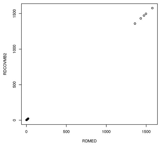
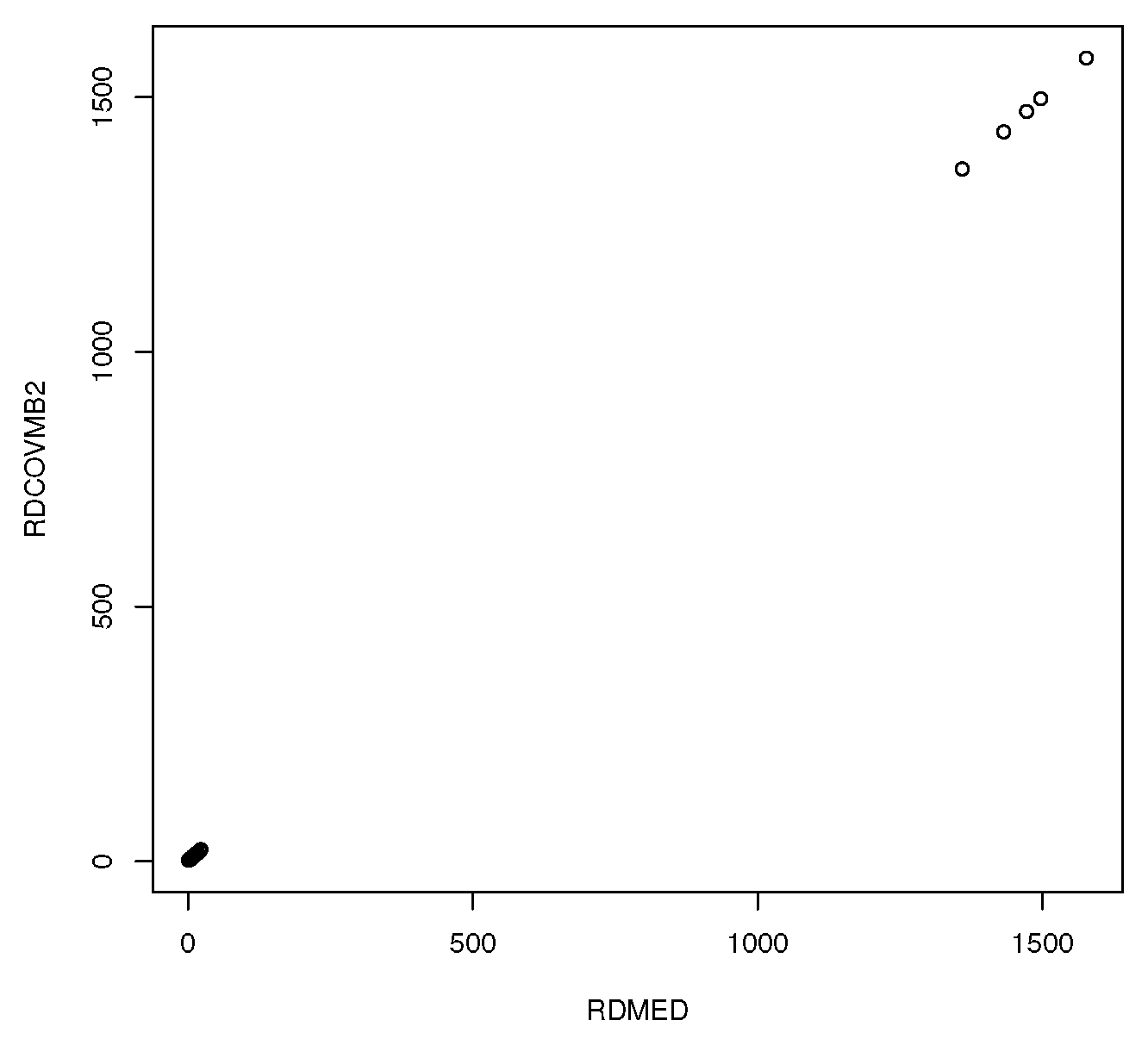
The function ddplot5 plots the Euclidean distances from the coordinatewise median versus the Euclidean distances from the covmb2 location estimator. Typically, the plotted points in this DD plot cluster about the identity line, and outliers appear in the upper right corner of the plot with a gap between the bulk of the data and the outliers.

3. Results

Example 1. 

For the [43] data with multiple linear regression, height was the response variable, while an intercept, head length, nasal height, bigonal breadth, and cephalic index were used as predictors in the multiple linear regression model. Observation 9 was deleted, since it had missing values. Five individuals, cases 61–65, were reported to be about 0.75 inches tall with head lengths well over five feet. When the covmb2 set B was applied to the predictors, the set B included all of the clean cases and omitted the 5 outliers, making almost any reasonable multiple linear regression estimator outlier resistant for this data set. Figure 1 shows the DD plot made using ddplot5. The five outliers are in the upper right corner.

Figure 1. The outliers are in the upper right corner of the DD Plot.

Example 2. 

For the pollution data of [44], the response $Y=mort$ is the mortality rate, and most of the predictors were related to pollution. The full model used $n=60$ cases and $p=16$ predictors including a constant. The response and residual plots were good. Notice that $n=60<5p.$ Table 1 gives ${\widehat{\mathit{\beta }}}_{OLS}$ along with the standard errors for the ${\widehat{\beta }}_i$. Backwards elimination with the $C_p$ criterion with OLS used six predictors: a constant, EDUC, JANT, log(NONW), log(NOX), and PREC. Also shown are the [1] Liu estimator using ridge regression with $k=2=-d$, ridge regression with $k=2$, the [8] estimator with $k=2$, and the [3] Liu estimator using OLS and $c=0.5$. The predictors are highly correlated with $n=60$ small. Hence, even with $k=\lfloor n^{1/4}\rfloor =2$, the estimated coefficients differ considerably. The ridge regression and two Liu estimates do appear somewhat similar. The fitted values from these three estimators and the OLS full model were highly correlated.

Table 1. Estimators for pollution data.

	OLS	OLS SE	Liu, $\mathit{k}=-\mathit{d}$	RR, $\mathit{k}=2$	KL, $\mathit{k}=2$	Liu, $\mathit{c}=0.5$
Constant	1881.11	442.6280	16.7700	8.8414	$-1863.430$	948.6509
DENS	0.0030	0.0040	0.0041	0.0039	0.0048	0.0035
EDUC	$-19.6669$	10.7005	$-2.3136$	$-1.4804$	16.7060	$-10.8567$
log[HC]	$-31.0112$	15.5615	$-5.4309$	$-0.1439$	30.7235	$-17.4127$
HOUS	$-0.4011$	1.6437	2.3359	2.6368	5.6747	0.9886
HUMID	$-0.4454$	1.0676	1.8651	2.1661	4.7775	0.7464
JANT	$-3.5852$	1.0536	$-3.0178$	$-3.2059$	$-2.8266$	$-3.3087$
JULT	$-3.8429$	2.1208	3.1104	3.8312	11.5054	$-0.2799$
log[NONW]	27.2397	10.1340	24.7506	20.6156	13.9916	25.2578
log[NOX]	57.3041	15.4764	30.1645	24.3417	$-8.6207$	42.7146
OVR65	$-15.9444$	8.0816	4.5711	2.4327	20.8098	$-6.0297$
POOR	3.41434	2.7475	5.5791	6.2031	8.9919	4.5624
POPN	$-131.8230$	69.1908	50.5519	29.1208	190.0642	$-42.9320$
PREC	3.6714	0.7781	2.5125	2.5911	1.5108	3.1020
log[SO]	$-10.2973$	7.3820	0.2036	2.4339	15.1651	$-4.6422$
WWDRK	0.8825	1.5095	0.3979	0.1416	$-0.5992$	0.6065

A useful application of the large-sample theory is to better understand the simulations in the literature. The simulations tend to give methods for choosing parameters, such as k and d, for some quantity of interest, including (a) the MSE of ${\widehat{\mathit{\beta }}}_i$ or (b) confidence intervals for ${\beta }_i$. For (a), it is important that $k/\sqrt{n}\to 0$ and $d/\sqrt{n}\to 0$ so that asymptotic normality and $\sqrt{n}$ consistency of the estimator is not lost. For (b), the simulations for confidence intervals assume asymptotic normality without proof.

Suppose $\sqrt{n}(\widehat{\mathit{\beta }}-\mathit{\beta })\stackrel{D}{\to }{N}_p(\mathbf{0},\mathit{D})$ and that $\widehat{\mathit{D}}$ is a consistent nonsingular estimator of $\mathit{D}$. Let ${\mathit{\beta }}_I={({\beta }_{i_1},\dots ,{\beta }_{i_g})}^T$. Then $\sqrt{n}({\widehat{\mathit{\beta }}}_I-{\mathit{\beta }}_I)\stackrel{D}{\to }{N}_g(\mathbf{0},{\mathit{D}}_I)$, where ${\mathit{D}}_I$ has the rows and columns of $\mathit{D}$ corresponding to $I=\{i_1,\dots ,i_g\}$. Then ${({\widehat{\mathit{\beta }}}_I-{\mathit{\beta }}_I)}^T{\widehat{\mathit{D}}}_I^{-1}({\widehat{\mathit{\beta }}}_I-{\mathit{\beta }}_I)\stackrel{D}{\to }{\chi }_g^2$ as $n\to \infty$. Since $g{F}_{g,n-p}\stackrel{D}{\to }{\chi }_g^2$, a $100(1-\delta )$% confidence region for ${\mathit{\beta }}_I$ is

$$\{{\mathit{\beta }}_I:{({\widehat{\mathit{\beta }}}_I-{\mathit{\beta }}_I)}^T{\widehat{\mathit{D}}}_I^{-1}({\widehat{\mathit{\beta }}}_I-{\mathit{\beta }}_I)\le g{F}_{g,n-p,1-\delta }\},$$

where $P(X\le F_{g,n-p,1-\delta })=1-\delta$ when $X\sim F_{g,n-p}$. The scaled F distribution cutoff $g{F}_{g,n-p,1-\delta }$ could be replaced by the chi-square distribution cutoff ${\chi }_{g,1-\delta }^2$. Consider the test $H_0:{\mathit{\beta }}_I={\mathit{\beta }}_{I,0}$ versus $H_1:{\mathit{\beta }}_I\ne {\mathit{\beta }}_{I,0}$. Then for a level $\delta$ test, fail to reject $H_0$ if ${\mathit{\beta }}_{I,0}$ is in the $100(1-\delta )$% confidence region for ${\mathit{\beta }}_I$, and reject $H_0$ otherwise.

To derive a confidence interval (CI) for ${\beta }_i$, note that $\sqrt{n}({\widehat{\beta }}_i-{\beta }_i)\stackrel{D}{\to }N(0,D_{ii})$ where $D_{ii}$ is the ith diagonal element of $\mathit{D}$. Hence the standard error $SE\left({\widehat{\beta }}_i\right)=\sqrt{{\widehat{D}}_{ii}}/\sqrt{n}$, and a $100(1-\delta )$% CI for ${\beta }_i$ is ${\widehat{\beta }}_i\pm t_{n-p,1-\delta /2}SE\left({\widehat{\beta }}_i\right).$ For a 95% CI, $t_{n-p,1-\delta /2}\to 1.96$ as $n\to \infty$.

For multiple linear regression with OLS and ridge-type estimators, $\mathit{D}={\sigma }^2\mathit{V}$ and $\widehat{\mathit{D}}=MSEn{\left({\mathit{X}}^T\mathit{X}\right)}^{-1}.$ Hence $SE\left({\widehat{\beta }}_i\right)=\sqrt{MSE}\sqrt{{\widehat{v}}_{ii}}$, where ${\widehat{v}}_{ii}$ is the ith diagonal element of ${\left({\mathit{X}}^T\mathit{X}\right)}^{-1}$. Then use $\widehat{\mathit{\beta }}$ in place of ${\widehat{\mathit{\beta }}}_{OLS}$ where $\widehat{\mathit{\beta }}$ satisfies Theorem 1 (a) (i) or Theorem 2 (a). For example, if $[L,U]$ is the $100(1-\delta )$% CI for ${\beta }_i$ using OLS, then

$$[L-{\widehat{\beta }}_{i,OLS}+{\widehat{\beta }}_i,U-{\widehat{\beta }}_{i,OLS}+{\widehat{\beta }}_i]$$

(11)

is a $100(1-\delta )$% CI for ${\beta }_i$ using $\widehat{\mathit{\beta }}={({\widehat{\beta }}_1,\dots ,{\widehat{\beta }}_p)}^T$. Other estimators of $\widehat{\mathit{D}}$ can be used.

We performed a small simulation for MLR using the estimators in Table 1. Let $\mathit{x}={\left(1{\mathit{u}}^T\right)}^T$ where $\mathit{u}$ is the $(p-1)\times 1$ vector of nontrivial predictors. Let $Y=\alpha +{\mathit{\varphi }}^T\mathit{u}+e$ with $\mathit{\beta }={(\alpha ,{\mathit{\varphi }}^T)}^T$. In the simulations, for $i=1,\dots ,n$, we generated ${\mathit{w}}_i\sim N_{p-1}(\mathbf{0},\mathit{I})$ where the $m=p-1$ elements of the vector ${\mathit{w}}_i$ are independent and identically distributed N(0,1). Let the $m\times m$ matrix $\mathit{A}=\left(a_{ij}\right)$ with $a_{ii}=1$ and $a_{ij}=\psi$ where $0\le \psi <1$ for $i\ne j$. Then the vector ${\mathit{u}}_i=\mathit{A}{\mathit{w}}_i$ so that $Cov\left({\mathit{u}}_i\right)={\Sigma }_{\mathit{u}}=\mathit{A}{\mathit{A}}^T=\left({\sigma }_{ij}\right)$ where the diagonal entries ${\sigma }_{ii}=[1+(m-1){\psi }^2]$ and the off diagonal entries ${\sigma }_{ij}=[2\psi +(m-2){\psi }^2]$. Hence the correlations are $cor(x_i,x_j)=\rho =(2\psi +(m-2){\psi }^2)/(1+(m-1){\psi }^2)$ for $i\ne j$, where $x_i$ and $x_j$ are nontrivial predictors. If $\psi =1/\sqrt{cp}$, then $\rho \to 1/(c+1)$ as $p\to \infty$ where $c>0$. As  $\psi$ gets close to 1, the predictor vectors cluster about the line in the direction of ${(1,\dots ,1)}^T.$ Let $Y_i=1+1x_{i,2}+\cdots +1x_{i,p}+e_i$ for $i=1,\dots ,n$. Hence $\alpha =1$ and $\mathit{\beta }={(1,\dots ,1)}^T$.

The zero mean iid errors $e_i$ were iid from five distributions: (i) N(0,1), (ii) $t_3$, (iii) EXP(1)-1, (iv) uniform($-1,1$), and  (v) 0.9 N(0,1) + 0.1 N(0,100). Only distribution (iii) is not symmetric.

When $\psi =0$, the OLS 95% confidence intervals for ${\beta }_i$ should have length near $2t_{96,0.975}\sigma /\sqrt{n}$. Hence the scaled CI length = $\sqrt{n}$ CI length $\approx 2\left(1.96\right)\sigma =3.92\sigma$ when the iid zero mean errors have variance ${\sigma }^2$. These values are 3.92 for N(0,1) errors and 2.2632 for $U(-1,1)$ errors. The simulation gave the average scaled CI lengths: for $\psi =0$, Table 2 had lengths near 4.03, while Table 3 had lengths near 2.34. The simulation computed the large sample 95% CIs $[L_{in},U_{in}]$ for ${\beta }_i$ and $i=1,\dots ,p$. The test for $H_0:{({\beta }_1,{\beta }_2)}^T={(1,1)}^T$ was also performed. In total, 5000 CIs were generated for each ${\beta }_i$, and the coverage was the proportion of times ${\beta }_i$ was in its CI. Hence, if ${\beta }_1$ was in its interval 4750/5000 = 0.95, then the observed coverage was 0.95. With 5000 runs, coverage $\in [0.94,0.96]$ gives no reason to doubt that the nominal coverage is 0.95. The average scaled lengths of the CIs are the same for each of the five estimators, but the coverages could differ. No length is available for the confidence region corresponding to the column headed by testcov. We used $p=4$ and $n=100$. Table 2 shows results for N(0,1) errors while Table 3 uses $U(-1,1)$ errors. With $k=\sqrt{n}=10$ and $\tau =1$, the OLS-type asymptotics only work for the fourth ridge-type estimator: the Liu-type estimator with $k=-d$. See Theorem 1 (a) (ii). The other three ridge-type estimators did not estimate the constant well. Two of these three estimators estimated the slopes well when $\psi =0.5$, but not when $\psi =0$. With $k=n^{1/4}=3.162$ and $\tau =0$ asymptotically, the OLS-type asymptotics apply to all four ridge-type estimators.

Table 2. n = 100, p = 4, N(0,1) errors.

psi	$\mathit{k}=\mathit{c}$	rrtype	${\mathit{\beta }}_1$	${\mathit{\beta }}_2$	${\mathit{\beta }}_3$	${\mathit{\beta }}_4$	testcov
0	3.162	OLS	0.9480	0.9446	0.9526	0.9536	0.9494
0	3.162	RR	0.9434	0.9434	0.9488	0.9436	0.9412
0	3.162	KL	0.9150	0.9196	0.9198	0.9198	0.9076
0	3.162	Liu	0.9410	0.9366	0.9430	0.9398	0.9320
0	3.162	$k=-d$	0.9478	0.9452	0.9524	0.9538	0.9502
	len		4.0194	4.0387	4.0507	4.0414
0.5	3.162	OLS	0.9480	0.9468	0.9528	0.9454	0.9500
0.5	3.162	RR	0.9436	0.9714	0.9752	0.9724	0.9584
0.5	3.162	KL	0.9182	0.9882	0.9870	0.9836	0.9572
0.5	3.162	Liu	0.9400	0.9278	0.9330	0.9300	0.9244
0.5	3.162	$k=-d$	0.9558	0.9546	0.9520	0.9548	0.9558
	len		4.0195	6.6969	6.7191	6.7043
0	10	OLS	0.9470	0.9518	0.9528	0.9508	0.9468
0	10	RR	0.8664	0.8670	0.8718	0.8734	0.8330
0	10	KL	0.5802	0.5618	0.5624	0.5438	0.3946
0	10	Liu	0.8254	0.8270	0.8280	0.8294	0.7658
0	10	$k=-d$	0.9472	0.9520	0.9458	0.9490	0.9518
	len		4.0148	4.0394	4.0388	4.0416
0.5	10	OLS	0.9480	0.9468	0.9528	0.9454	0.9500
0.5	10	RR	0.8744	0.9896	0.9938	0.9904	0.9328
0.5	10	KL	0.5692	0.9990	0.9998	0.9996	0.7530
0.5	10	Liu	0.8262	0.8452	0.8550	0.8500	0.7904
0.5	10	$k=-d$	0.9486	0.9638	0.9702	0.9666	0.9612
	len		4.0194	6.6969	6.7190	6.7043

Table 3. n = 100, p = 4, U($-1$,1) errors.

psi	$\mathit{k}=\mathit{c}$	rrtype	${\mathit{\beta }}_1$	${\mathit{\beta }}_2$	${\mathit{\beta }}_3$	${\mathit{\beta }}_4$	testcov
0	3.162	OLS	0.9508	0.9500	0.9492	0.9434	0.9508
0	3.162	RR	0.9294	0.9238	0.9218	0.9204	0.9142
0	3.162	KL	0.8258	0.8230	0.8248	0.8200	0.7734
0	3.162	Liu	0.9320	0.9272	0.9282	0.9274	0.9232
0	3.162	$k=-d$	0.9514	0.9500	0.9490	0.9434	0.9508
	len		2.3262	2.3414	2.3437	2.3392
0.5	3.162	OLS	0.9508	0.9480	0.9426	0.9458	0.9488
0.5	3.162	RR	0.9280	0.9696	0.9686	0.9688	0.9454
0.5	3.162	KL	0.8300	0.9844	0.9840	0.9820	0.8988
0.5	3.162	Liu	0.9302	0.9252	0.9228	0.9262	0.9216
0.5	3.162	$k=-d$	0.9514	0.9510	0.9456	0.9478	0.9498
	len		2.3262	3.8852	3.8880	3.8801
0	10	OLS	0.9508	0.9500	0.9492	0.9434	0.9508
0	10	RR	0.6600	0.6600	0.6676	0.6644	0.5144
0	10	KL	0.1094	0.1076	0.1130	0.1086	0.0116
0	10	Liu	0.6412	0.6404	0.6332	0.6378	0.4992
0	10	$k=-d$	0.9504	0.9512	0.9474	0.9442	0.9482
	len		2.3262	2.3415	2.3437	2.3392
0.5	10	OLS	0.9508	0.9480	0.9420	0.9458	0.9488
0.5	10	RR	0.6700	0.9872	0.9874	0.9874	0.7870
0.5	10	KL	0.0834	0.9946	0.9960	0.9932	0.1828
0.5	10	Liu	0.6414	0.8384	0.8390	0.8348	0.6406
0.5	10	$k=-d$	0.9514	0.9656	0.9634	0.9640	0.9588
	len		2.3262	3.8852	3.8800	3.8801

Table 4 used $p=10$, $psi=0.9$, and EXP(1)-1 errors. Hence the predictors are highly correlated and the errors are not from a symmetric distribution. The confidence interval coverages were similar for ${\beta }_2$ to ${\beta }_{10}$ for each of the five regression estimators. Table 4 shows the confidence interval coverages for ${\beta }_1,{\beta }_2,{\beta }_9$, and  ${\beta }_{10}$. The test was $H_0:{({\beta }_2,{\beta }_4)}^T={(1,1)}^T.$ Hence the constant ${\beta }_1$ was not tested. The Liu estimator with $c=n^{1/4}$ performed poorly, but the performance did improve as n increased.

Table 4. The test used indices 2 and 4, p = 10, EXP(1)-1 errors.

n	psi	$\mathit{k}=\mathit{c}$	rrtype	${\mathit{\beta }}_1$	${\mathit{\beta }}_2$	${\mathit{\beta }}_9$	${\mathit{\beta }}_{10}$	testcov
81	0.9	3	OLS	0.9396	0.9518	0.9500	0.9576	0.9506
81	0.9	3	RR	0.9280	1.0	1.0	1.0	1.0
81	0.9	3	KL	0.8874	0.9968	0.9978	0.9978	0.9990
81	0.9	3	Liu	0.8982	0.6316	0.6244	0.6360	0.4722
81	0.9	3	$k=-d$	0.9566	1.0	1.0	1.0	1.0
81	0.9		len	4.1932	39.8936	39.8962	39.9613
2410	0.9	7	OLS	0.9498	0.9500	0.9546	0.9462	0.9530
2410	0.9	7	Liu	0.9490	0.8910	0.8960	0.8770	0.8662
2410	0.9	7	len	3.9282	37.0673	37.04269	37.05407

The simulation can be replicated using R code such as that shown below.

source(“http://parker.ad.siu.edu/Olive/slpack.txt”)

#rrtype=1 for RR, 2 for KL, 3 for Liu, 4 for Liu k=-d

#error type=1 for N(0,1), 2 for t_3,  3 for EXP(1) - 1,

#4 for uniform(-1,1), 5 for (1-eps) N(0,1) + eps N(0,(1+shift)^2)

set.seed(970)

mlrcisim(psi=0.5,nruns=5000,rrtype=4,type=4,k=10)

set.seed(970)

mlrcisim(psi=0.5,nruns=5000,rrtype=3,type=4,c=10,k=10)

set.seed(970)

mlrcisim(psi=0.5,nruns=5000,rrtype=2,type=4,k=10)

set.seed(970)

mlrcisim(psi=0.5,nruns=5000,rrtype=1,type=4,k=10)

4. Discussion

Theorems 1–6 give a large-sample theory for many ridge-type estimators. The theorems give conditions for the ridge-type estimator to be asymptotically equivalent to the usual estimator ($k/\sqrt{n}\to 0$), where the asymptotic normality is inferior to that of the usual estimator ($k/\sqrt{n}\to \tau >0$) and where the ridge-type estimator is consistent ($k/n\to 0)$.

Taking $d=-k$ is interesting in Theorem 1. Several of the ridge-type estimators can be computed if $k>0$ even if ${\mathit{X}}^T\mathit{X}$ is singular, and such estimators can be useful if $p>n$. Ref. [45] gave a Liu-type estimator that replaced $\widehat{\mathit{\beta }}$ by a vector $\mathit{b}$ that represents prior information. Ref. [46] gave more ridge-type estimators. Ref. [47] considers ridge-type models for the partial linear regression model.

Define ${\widehat{\mathit{\beta }}}_k={({\mathit{X}}^T\mathit{X}+k{\mathit{I}}_p)}^{-1}({\mathit{X}}^T\mathit{Y}+k{\widehat{\mathit{\beta }}}_{R,k})$ to be the estimator from Theorem 1 (a) (ii). Ref. [48] (pp. 381–382, 392) shows that ${\widehat{\mathit{\beta }}}_{R,k}={\mathit{X}}^T{(\mathit{X}{\mathit{X}}^T+k{\mathit{I}}_n)}^{-1}\mathit{Y}.$ Hence ${\widehat{\mathit{\beta }}}_k={({\mathit{X}}^T\mathit{X}+k{\mathit{I}}_p)}^{-1}{\mathit{X}}^T\mathit{Z}={\widehat{\mathit{\beta }}}_{R,k}\left(\mathit{Z}\right)$ where ${\widehat{\mathit{\beta }}}_{R,k}\left(\mathit{Z}\right)$ is the ridge regression estimator from regressing $\mathit{Z}$ on $\mathit{X}$, and $\mathit{Z}=\mathit{Y}+k{(\mathit{X}{\mathit{X}}^T+k{\mathit{I}}_n)}^{-1}\mathit{Y}$. Hence ${\widehat{\mathit{\beta }}}_k={\mathit{X}}^T{(\mathit{X}{\mathit{X}}^T+k{\mathit{I}}_n)}^{-1}\mathit{Z}$, which can be quick to compute if n is much smaller than p.

When $\sqrt{n}$ consistent estimators are used,

$$\parallel {\widehat{\mathit{\beta }}}_E-{\mathit{\beta }}_E{\parallel }^2={\displaystyle \sum _{i=1}^p}{({\widehat{\beta }}_i-{\beta }_i)}^2\propto {\displaystyle \frac{p}{n}}.$$

In low dimensions where p is fixed, $p/n\to 0$ as $n\to \infty$ and ${\widehat{\mathit{\beta }}}_E$ is a consistent estimator. In high dimensions, $\parallel {\widehat{\mathit{\beta }}}_E-{\mathit{\beta }}_E{\parallel }^2$ tends to not be close to 0. For example, if $p=p_n=n^{\tau +1}$, then $p_n/n=n^{\tau }$ which tends to be large if n is large and $\tau >1$. Hence, in high dimensions, it is difficult to get a good estimator ${\widehat{\mathit{\beta }}}_E$ of ${\mathit{\beta }}_E$.

Ref. [49] has an interesting result for the second multiple linear regression model (9). Assume that the cases ${({\mathit{x}}_i^T,Y_i)}^T$ are iid with $E\left(Y\right)={\mu }_Y$, $E\left(\mathit{x}\right)={\mathit{\mu }}_{\mathit{x}}$ and nonsingular $Cov\left(\mathit{x}\right)={\Sigma }_{\mathit{x}}$. Then testing $H_0:\mathit{\beta }={\mathit{\beta }}_0$ versus $H_1:\mathit{\beta }\ne {\mathit{\beta }}_0$ is equivalent to testing $H_0:\mathit{\mu }=\mathbf{0}$ versus $H_1:\mathit{\mu }\ne \mathbf{0}$ with $\mathit{\mu }=E\left({\mathit{z}}_i\right)={\Sigma }_{\mathit{x}}(\mathit{\beta }-{\mathit{\beta }}_0)$ where ${\mathit{z}}_i=({\mathit{x}}_i-{\mathit{\mu }}_{\mathit{x}})(Y_i-{\mu }_Y-{({\mathit{x}}_i-{\mathit{\mu }}_{\mathit{x}})}^T{\mathit{\beta }}_0)$, and a high dimensional one-sample test can be applied to ${\mathit{v}}_i=({\mathit{x}}_i-\overline{\mathit{x}})(Y_i-\overline{Y}-{({\mathit{x}}_i-\overline{\mathit{x}})}^T{\mathit{\beta }}_0).$ Since $\mathit{\beta }={\mathit{\beta }}_{OLS}={\Sigma }_{\mathit{x}}^{-1}{\Sigma }_{\mathit{x}Y}$ and $\mathit{\beta }=\mathbf{0}$ if and only if $Cov(\mathit{x},Y)={\Sigma }_{\mathit{x}Y}=\mathbf{0}$, using ${\mathit{\beta }}_0=\mathbf{0}$ gives high-dimensional tests for $H_0:\mathit{\beta }=\mathbf{0}$ and $H_0:{\Sigma }_{\mathit{x}Y}=\mathbf{0}$. Ref. [50] proved that the high-dimensional test for $H_0:\mathit{\beta }=\mathbf{0}$ also works for GLMs.

The R software was used. See [51]. Programs are available from the collection of R functions slpack.txt, available from (http://parker.ad.siu.edu/Olive/slpack.txt (accessed on 17 June 2026)).

The covmb2 estimator attempts to give a robust dispersion estimator that reduces bias by using a big ball about ${\mathrm{MED}}_j$ instead of a ball that contains half of the cases. The median ball is the hypersphere centered at the coordinatewise median with radius $r=\mathrm{MED}(D_i(\mathrm{MED}\left(\mathit{W}\right),{\mathit{I}}_p),i=1,\dots ,n)$ that tends to contain $(n+1)/2$ of the cases if n is odd. The slpack function getB gives the set B of cases that got weight 1 along with the index indx of the case numbers that got weight 1. Example 2 used the function ridgetype. The function mlrcisim was used for Table 2, Table 3 and Table 4.

Ridge-type estimators ${\widehat{\mathit{\beta }}}_{RMLE}={({\mathit{X}}^T\widehat{\mathit{W}}\mathit{X}+k{\mathit{I}}_p)}^{-1}\left({\mathit{X}}^T\widehat{\mathit{W}}\mathit{X}\right){\widehat{\mathit{\beta }}}_{MLE}$ are used for quality control charts. See, for example, [52]. These estimators have the same large sample theory as that given in Theorem 5 with ${\widehat{\mathit{\beta }}}_{MLE}$ replacing ${\widehat{\mathit{\beta }}}_{GLM}.$

References

- Liu, K. Using Liu-type estimator to combat collinearity. Commun. Stat. Theory Methods 2003, 32, 1009–1020. [Google Scholar] [CrossRef] [Scilit]
- Hoerl, A.E.; Kennard, R. Ridge regression: Biased estimation for nonorthogonal problems. Technometrics 1970, 12, 55–67. [Google Scholar] [CrossRef]
- Liu, K. A new class of biased estimate in linear regression. Commun. Stat. Theory Methods 1993, 22, 393–402. [Google Scholar]
- Kurnaz, F.S.; Akay, K.U. A new Liu-type estimator. Stat. Pap. 2015, 56, 495–517. [Google Scholar]
- Özkale, M.R.; Kaçiranlar, S. The restricted and unrestricted two-parameter estimators. Commun. Stat. Theory Methods 2007, 36, 2707–2725. [Google Scholar] [CrossRef] [Scilit]
- Sakallioǧlu, S.; Kaçiranlar, S. A new biased estimator based on ridge estimation. Stat. Pap. 2008, 49, 669–689. [Google Scholar]
- Yang, H.; Chang, X. A new two-parameter estimator in linear regression. Commun. Stat. Theory Methods 2010, 39, 923–934. [Google Scholar] [CrossRef] [Scilit]
- Kibria, B.M.G.; Lukman, A.F. A new ridge-type estimator for the linear regression model: Simulations and applications. Scientifica 2020, 2020, 9758378. [Google Scholar] [CrossRef] [Scilit] [PubMed]
- Sen, P.K.; Singer, J.M. Large Sample Methods in Statistics: An Introduction with Applications; Chapman & Hall: New York, NY, USA, 1993. [Google Scholar]
- Knight, K.; Fu, W.J. Asymptotics for lasso-type estimators. Ann. Stat. 2000, 28, 1356–1378. [Google Scholar] [CrossRef] [Scilit]
- Tibshirani, R. Regression shrinkage and selection via the lasso. J. Roy. Stat. Soc. B 1996, 58, 267–288. [Google Scholar] [CrossRef] [Scilit]
- Gunst, R.F.; Mason, R.L. Regression Analysis and Its Application; Marcel Dekker: New York, NY, USA, 1980. [Google Scholar]
- Pelawa Watagoda, L.C.R.; Olive, D.J. Comparing six shrinkage estimators with large sample theory and asymptotically optimal prediction intervals. Stat. Pap. 2021, 62, 2407–2431. [Google Scholar]
- Ertaş, H. A modified ridge M-estimator for linear regression model with multicollinearity and outliers. Commun. Stat. Simul. Comput. 2018, 47, 1240–1250. [Google Scholar]
- Haider, B.; Asim, S.M.; Wasim, D.; Kibria, B.G.M. A simulation-based comparative analysis of two parameter robust ridge M-estimators for linear regression model. Stats 2025, 8, 84. [Google Scholar]
- Majid, A.; Amin, M.; Aslam, M.; Ahmad, S. New robust ridge estimators for the linear regression model with outliers. Commun. Stat. Simul. Comput. 2023, 52, 4717–4738. [Google Scholar]
- Sivapulle, M.J. Robust ridge regression based on an M-estimator. Aust. J. Stat. 1991, 33, 319–333. [Google Scholar]
- Bassett, G.W.; Koenker, R.W. Asymptotic theory of least absolute error regression. J. Am. Stat. Assoc. 1978, 73, 618–622. [Google Scholar] [CrossRef]
- Zhou, L.; Cook, R.D.; Zou, H. Enveloped Huber regression. J. Am. Stat. Assoc. 2024, 119, 2722–2732. [Google Scholar]
- Nelder, J.A.; Wedderburn, R.W.M. Generalized linear models. J. R. Stat. Soc. Ser. A 1972, 135, 370–384. [Google Scholar] [CrossRef] [Scilit]
- Hillis, S.L.; Davis, C.S. A simple justification of the iterative fitting procedure for generalized linear models. Am. Stat. 1994, 48, 288–289. [Google Scholar] [CrossRef] [Scilit]
- Agresti, A. Categorical Data Analysis, 2nd ed.; Wiley: Hoboken, NJ, USA, 2002. [Google Scholar]
- Schaefer, R.L.; Roi, L.D.; Wolfe, R.A. A ridge logistic estimator. Commun. Stat. Theory Methods 1984, 13, 99–113. [Google Scholar] [CrossRef] [Scilit]
- Månsson, K.; Shukur, G. On ridge parameters in logistic regression. Commun. Stat. Theory Methods 2011, 40, 3366–3381. [Google Scholar] [CrossRef] [Scilit]
- Månsson, K.; Shukur, G. A Poisson ridge regression estimator. Econ. Model. 2011, 28, 1475–1481. [Google Scholar] [CrossRef] [Scilit]
- Chowdhury, S.M.R.; Bursac, Z.; Kibria, B.M.G. Improving confidence interval estimation in logistic regression with multicollinear predictors: A comparative study of shrinkage estimators and application to prostate cancer data. Stats 2026, 9, 11. [Google Scholar] [CrossRef] [Scilit]
- Månsson, K.; Kibria, B.M.G.; Shukur, G. On Liu estimators for the logit regression model. Econ. Model. 2012, 29, 1483–1488. [Google Scholar] [CrossRef] [Scilit]
- Ertan, E.; Akay, K.U. A new class of Poisson ridge-type estimator. Sci. Rep. 2023, 13, 4968. [Google Scholar] [CrossRef] [Scilit] [PubMed]
- Crivelli, A.; Firinguetti, L.; Montano, R.; Munóz, M. Confidence intervals in ridge regression by bootstrapping the dependent variable: A simulation study. Commun. Stat. Simul. Comput. 1995, 24, 631–652. [Google Scholar] [CrossRef] [Scilit]
- Cule, E.; Vineis, P.; De Iorio, M. Significance testing in ridge regression for genetic data. BMC Bioinform. 2011, 12, 372. [Google Scholar] [CrossRef] [Scilit]
- Halawa, A.M.; El Bassiouni, M.Y. Tests of regression coefficients under ridge regression models. J. Stat. Comput. Simul. 2000, 65, 341–356. [Google Scholar] [CrossRef] [Scilit]
- Özkale, M.R.; Altuner, H. Bootstrap confidence interval of ridge regression in linear regression model: A comparative study via a simulation study. Commun. Stat. Theory Methods 2023, 52, 7405–7441. [Google Scholar]
- Akaike, H. Information theory and an extension of the maximum likelihood principle. In Proceedings of the 2nd International Symposium on Information Theory; Petrov, B.N., Csakim, F., Eds.; Akademiai Kiado: Budapest, Hungary, 1973; pp. 267–281. [Google Scholar]
- Schwarz, G. Estimating the dimension of a model. Ann. Stat. 1978, 6, 461–464. [Google Scholar] [CrossRef] [Scilit]
- Chen, J.; Chen, Z. Extended Bayesian information criterion for model selection with large model spaces. Biometrika 2008, 95, 759–771. [Google Scholar] [CrossRef] [Scilit]
- Mallows, C. Some comments on Cp. Technometrics 1973, 15, 661–676. [Google Scholar]
- James, G.; Witten, D.; Hastie, T.; Tibshirani, R. An Introduction to Statistical Learning with Applications in R, 2nd ed.; Springer: New York, NY, USA, 2021. [Google Scholar]
- Meinshausen, N. Relaxed lasso. Comput. Stat. Data Anal. 2007, 52, 374–393. [Google Scholar] [CrossRef] [Scilit]
- Bülmann, P.; van de Geer, S. Statistics for High-Dimensional Data Methods, Theory and Applications; Springer: New York, NY, USA, 2011. [Google Scholar]
- Olive, D.J.; Hawkins, D.M. Variable selection for 1D regression models. Technometrics 2005, 47, 43–50. [Google Scholar] [CrossRef] [Scilit]
- Rathnayake, R.C.; Olive, D.J. Bootstrapping some GLMs and survival regression models after variable selection. Commun. Stat. Theory Methods 2023, 52, 2625–2645. [Google Scholar]
- Olive, D.J. Robust Multivariate Analysis; Springer: New York, NY, USA, 2017. [Google Scholar]
- Buxton, L.H.D. The anthropology of Cyprus. J. Anthropol. Inst. Great Br. Irel. 1920, 50, 183–235. [Google Scholar] [CrossRef] [Scilit]
- McDonald, G.C.; Schwing, R.C. Instabilities of regression estimates relating air pollution to mortality. Technometrics 1973, 15, 463–482. [Google Scholar] [CrossRef] [Scilit]
- Li, Y.; Yang, H. A new Liu-type estimator in linear regression model. Stat. Pap. 2012, 53, 427–437. [Google Scholar]
- Sidhu, B.K.; Tiwari, M.K.; Bist, V.; Kumar, M.; Pathak, A. A new modified generalized two parameter estimator for linear regression model. Commun. Stat. Theory Methods 2025, 54, 2807–2826. [Google Scholar]
- Arashi, M.; Valizadeh, T. Performance of Kibria’s methods in partial linear ridge regression model. Stat. Pap. 2015, 56, 231–246. [Google Scholar]
- Efron, B.; Hastie, T. Computer Age Statistical Inference; Cambridge University Press: New York, NY, USA, 2016. [Google Scholar]
- Zhao, A.; Li, C.; Li, R.; Zhang, Z. Testing high-dimensional regression coefficients in linear models. Ann. Stat. 2024, 52, 2034–2058. [Google Scholar] [CrossRef] [Scilit] [PubMed]
- Abid, A.M.; Quaye, P.A.; Olive, D.J. A high dimensional omnibus regression test. Stats 2025, 8, 107. [Google Scholar] [CrossRef] [Scilit]
- R Core Team. R: A Language and Environment for Statistical Computing; R Foundation for Statistical Computing: Vienna, Austria, 2024. [Google Scholar]
- Amin, M.; Rani, S.; Aljeddani, S.M.A. Pearson and deviance residual-based control charts for the inverse Gaussian ridge regression process: Simulation and an application to air quality monitoring. Axioms 2025, 14, 455. [Google Scholar] [CrossRef] [Scilit]
Disclaimer/Publisher’s Note: The statements, opinions and data contained in all publications are solely those of the individual author(s) and contributor(s) and not of MDPI and/or the editor(s). MDPI and/or the editor(s) disclaim responsibility for any injury to people or property resulting from any ideas, methods, instructions or products referred to in the content. |
© 2026 by the authors. Licensee MDPI, Basel, Switzerland. This article is an open access article distributed under the terms and conditions of the Creative Commons Attribution (CC BY) license.