The Generalized Marshall–Olkin Topp–Leone-G Family: Properties, Estimation, and Goodness-of-Fit Testing Under Right-Censored Data

Abstract

In this paper, we introduce a new extension of the Topp–Leone-G family, called the generalized Marshall–Olkin Topp–Leone-G (GMOTL-G) family of distributions. The proposed family is obtained by combining the generalized Marshall–Olkin and Topp–Leone-G generators, leading to a more flexible class of models for lifetime data. We study several of its mathematical and statistical properties and focus in particular on the generalized Marshall–Olkin Topp–Leone exponential (GMOTL-E) distribution as an important special case. For this model, we derive and discuss a number of useful characteristics, including the moment generating function, moments, order statistics, residual and reversed residual life functions, mean deviations, asymptotic behavior, and stochastic ordering. We also develop maximum likelihood estimation for the model parameters under both complete and right-censored samples. In addition, we construct a goodness-of-fit test for the proposed model under independent right censoring using a chi-square type approach. The performance of the estimation and testing procedures is investigated through simulation, and the results show good behavior of the estimators and satisfactory agreement between empirical and theoretical significance levels. Finally, two real data applications, one with complete data and one with right-censored data, are presented to illustrate the flexibility and practical usefulness of the proposed model. These results show that the new family provides an effective tool for modeling lifetime data and for assessing model adequacy in the presence of right censoring.

1. Introduction

In recent years, there has been growing interest in developing flexible families of probability distributions for modeling lifetime and reliability data. This is mainly because classical distributions are often not flexible enough to describe the different patterns observed in real data, especially when the data are skewed, heavy-tailed, or associated with hazard rate functions of various shapes.In many practical applications such as survival analysis, reliability engineering, medicine, and actuarial science, it is important to use models that can adequately capture different data behaviors; see Gross and Clark (1975) [1,2], it is important to use models that can capture these features adequately. For this reason, many authors have introduced new generators and extensions of existing distributions in order to obtain more adaptable models Several generalized lifetime models have therefore been proposed in the literature to improve flexibility and goodness-of-fit for complex data structures [3].

One of the most important and widely used generators in this direction is the Marshall–Olkin family, introduced by Marshall and Olkin (1997) [4]. This family provides a simple and effective way to add an extra parameter to a baseline distribution and improve its flexibility. Different extensions and applications of the Marshall–Olkin approach have been investigated in recent years for reliability and survival analysis problems [5]. Later, Jayakumar and Mathew (2008) [6] proposed the generalized Marshall–Olkin family, which extends the original idea by adding another shape parameter. This generalization gives more control over the tail behavior and the hazard rate function, and for that reason, it has attracted considerable attention in the literature.

$$S^{GMO}(t;\rho ,\delta )={\left[{\displaystyle \frac{\rho S\left(t\right)}{1-\overline{\rho }S\left(t\right)}}\right]}^{\delta }\mathrm{and}{f}^{GMO}(t;\rho ,\delta )={\displaystyle \frac{{\rho }^{\delta }\delta f\left(t\right)S{\left(t\right)}^{\delta -1}}{{\left[1-\overline{\rho }S\left(t\right)\right]}^{\delta +1}}}$$

(1)

where $-\infty <t<+\infty ,$ $\rho >0$ $\left(\overline{\rho }=1-\rho \right)$ and $\delta >0$ is an extra shape parameter. For $\delta =1$, the GMO family reduces to the MO family that is, $S^{GMO}(t;\rho ,\delta )=S^{MO}(t;\rho )$—and for $\delta =\rho =1$, the baseline model is $S^{GMO}(t;\rho ,\delta )=S\left(t\right).$

In 2016, Ali et al. [7], presented the Topp–Leone-G(TL-G) family. The TL-G family has attracted considerable attention because of its ability to generate flexible distributions with various hazard rate shapes [8]. Whose cdf and pdf are respectively

$$G^{TLG}\left(t;\omega \right)={\left[1-\overline{G}{\left(t\right)}^2\right]}^{\omega };t\in R,\omega >0$$

(2)

and

$$g^{TLG}(t;\omega )=2\omega g\left(t\right)\overline{G}\left(t\right){\left[1-\overline{G}{\left(t\right)}^2\right]}^{\omega -1}$$

(3)

where $g\left(x\right)$ represents the probability density function (pdf) and $\overline{G}\left(t\right)=1-G\left(t\right)$ denotes the survival function (sf) of the baseline distribution.

In addition to proposing a new distributional family, this paper is also concerned with statistical inference in the presence of right-censored data. Right censoring is very common in practice, especially in medical studies, reliability experiments, and survival analysis, where the exact lifetime may not be observed for all individuals or items under study. In such situations, the problem of assessing whether a proposed model fits the data well becomes more challenging. Although many generalized distributions have been introduced in the literature, relatively less attention has been given to goodness-of-fit procedures under right censoring Several authors have emphasized the importance of developing appropriate goodness-of-fit procedures for censored lifetime data [9] for these types of models. This motivates the second main aspect of the present work.

More precisely, the contribution of this paper is twofold. First, we introduce the GMOTL-G family and study its main structural and statistical properties. Second, we develop a goodness-of-fit testing procedure under right censoring for the proposed model by adapting the Bagdonavicius–Nikulin chi-square type approach. In this way, the paper is not limited to proposing a new model, but also addresses the important issue of model validation when censored observations are present.

To illustrate the proposed family in a concrete and useful way, we focus in particular on the generalized Marshall–Olkin Topp–Leone exponential (GMOTL-E) distribution, obtained by taking the exponential distribution as the baseline model. This special case is analytically convenient and practically relevant. Its density and hazard rate functions are derived explicitly, and the graphical results show that it is capable of exhibiting different shapes. We also study several of its properties, including moments, moment generating function, order statistics, residual life and reversed residual life functions, mean deviations, asymptotic behavior, and stochastic ordering. These results show that the proposed model is mathematically rich and potentially useful in applications.

From the inferential point of view, we develop maximum likelihood estimation for the model parameters under both complete and right-censored samples. Since the resulting likelihood equations are nonlinear, the estimates are obtained numerically. We then construct a goodness-of-fit test for right-censored data and apply it to the GMOTL-E model. The performance of the estimators and the proposed test is examined through simulation. In addition, two real data applications are considered in order to illustrate the usefulness of the model and compare it with some competing distributions.

The main objectives of this paper are therefore to introduce the GMOTL-G family by Mundher et al. (2020) [10], investigate its mathematical and statistical properties, study the GMOTL-E model as an important submodel, develop estimation procedures under complete and right-censored samples, and construct a goodness-of-fit test under right censoring. We believe that these contributions are relevant both from a theoretical point of view and from the perspective of practical statistical modeling.

The remainder of this paper is organized as follows. Section 2 introduces the generalized Marshall–Olkin Topp–Leone-G family and presents its main structural properties. Section 3 is devoted to the GMOTL-E model and some of its important statistical properties. Section 4 presents the inferential procedures, including maximum likelihood estimation and the goodness-of-fit test under right censoring. Section 5 contains the simulation study and the real data applications. Finally, the last section gives the conclusion and some possible directions for future work.

2. Proposed Generalized Marshall–Olkin Topp–Leone-G Family

Let $T_{i1},T_{i2},\dots T_{im}$ be a sequence of $\delta$ M $i.i.d$. random variables from $TL-G\left(\omega \right)$ distribution and suppose ${\vartheta }_i=min\left(T_{i1},T_{i2},\dots T_{im}\right)$ and ${\phi }_i=max\left(T_{i1},T_{i2},\dots T_{im}\right)$ for $i=1,2,\dots ,\delta$. We are interested in the distribution of ${\vartheta }_i$ and ${\phi }_i$.

Proof. 

Case I: If M possesses a geometric distribution with parameter $\rho$ $(0<\rho \le 1)$ independent of $T_i^{\prime }s$, then $\vartheta =min\left(T_1,T_2,\dots T_m\right)$ follows the $MOTL-G(\rho ,\omega )$ distribution.

For a specific M and $0<\rho <1,$

$$P(\vartheta >t)=P\left[min(t_1,t_2,\dots ,t_m)\right]=\prod ^{M}P(T_i>t)=\prod ^M{\left[S_T\left(t\right)\right]}^M$$

Let $M\backsim geo\left(\rho \right)$, then $P(M=u)={(1-\rho )}^{m-1}\rho ,$ $m=1,2,\dots$, and then

$$E{\left[S_T\left(t\right)\right]}^M={\displaystyle \sum _{m\ge 1}^{\infty }}{S}_T{\left(t\right)}^m{(1-\rho )}^{m-1}\rho =\rho S_T\left(t\right){\displaystyle \sum _{m\ge 1}^{\infty }}{S}_T{\left(t\right)}^{m-1}{(1-\rho )}^{m-1}={\displaystyle \frac{\rho S_T\left(t\right)}{1-\overline{\rho }{S}_T\left(t\right)}}$$

Now, $S_T\left(t\right)=1-{\left[1-\overline{G}{\left(t\right)}^2\right]}^{\omega }$, then

$$S_{\vartheta }\left(t\right)={\displaystyle \frac{\rho \left[1-{\left\{1-\overline{G}{\left(t\right)}^2\right\}}^{\omega }\right]}{1-\overline{\rho }\left[1-{\left\{1-\overline{G}{\left(t\right)}^2\right\}}^{\omega }\right]}}$$

If M has a geometric distribution with parameter $\rho$ $\left(0<\rho \le 1\right)$ independent of $T_{ij}^{\prime }s,$ then ${min}_{1\le i\le \delta }\left\{min\left(T_{i1},T_{i2},\dots T_{im}\right)\right\}$ is distributed as $GMOTL-G(\delta ,\rho ,\omega ).$

We have,

$$\begin{array}{ccc}\hfill P\left[min\left\{{\vartheta }_1,{\vartheta }_2,\dots ,{\vartheta }_{\delta }\right\}>t\right]& =& P\left[{\vartheta }_1>t\right]P\left[{\vartheta }_2>t\right]\dots \dots P\left[{\vartheta }_{\delta }>t\right]\hfill \\ & =& {\displaystyle \prod _{i=1}^{\delta }}P\left[{\vartheta }_i>t\right]={\left[S_{\vartheta }\left(t\right)\right]}^{\delta }\hfill \\ & =& {\left[{\displaystyle \frac{\rho \left[1-{\left\{1-\overline{G}{\left(t\right)}^2\right\}}^{\omega }\right]}{1-\overline{\rho }\left[1-{\left\{1-\overline{G}{\left(t\right)}^2\right\}}^{\omega }\right]}}\right]}^{\delta }\hfill \end{array}$$

Case II: If M has a geometric distribution with parameter $1/\rho$ $\left(\rho >1\right)$ independent of $T_i^{\prime }s$, then $\phi =max(T_1,T_2,\dots T_m)$ is distributed as $MOTL-G(\rho ,\omega )$.

For $\rho >1,$ $F_{\phi }\left(t\right)=P(\phi \le t)=P\left[T_i\le t,i=1,2,\dots ,M\right]=F_T{\left(t\right)}^M$.

Let $M\backsim geo(1/\rho )$, then $P(M=u)={(1-{\displaystyle \frac{1}{\rho }})}^{m-1}{\displaystyle \frac{1}{\rho }},$ $m=1,2,\dots$

$$\begin{array}{ccc}\hfill F_{\phi }\left(t\right)& =& E_M{\left[F_T\left(t\right)\right]}^M={\displaystyle \sum _{m\ge 1}^{\infty }}{F}_T{\left(t\right)}^m{(1-{\displaystyle \frac{1}{\rho }})}^{m-1}{\displaystyle \frac{1}{\rho }}\hfill \\ & =& {\displaystyle \frac{1}{\rho }}{F}_T\left(t\right){\displaystyle \sum _{m\ge 1}^{\infty }}{F}_T{\left(t\right)}^{m-1}{(1-{\displaystyle \frac{1}{\rho }})}^{m-1}={\displaystyle \frac{\frac{1}{\rho }{F}_T\left(t\right)}{1-\left(1-\frac{1}{\rho }\right)F_T\left(t\right)}}\hfill \end{array}$$

Now

$$\begin{array}{ccc}\hfill S_{\phi }\left(t\right)& =& 1-{\displaystyle \frac{\frac{1}{\rho }{F}_T\left(t\right)}{1-\left(1-\frac{1}{\rho }\right)F_T\left(t\right)}}={\displaystyle \frac{1-F_T\left(t\right)}{1-\left(1-\frac{1}{\rho }\right)F_T\left(t\right)}}={\displaystyle \frac{S_T\left(t\right)}{S_T\left(t\right)+\left(\frac{1}{\rho }\right)F_T\left(t\right)}}\hfill \\ & =& {\displaystyle \frac{\rho S_T\left(t\right)}{\rho S_T\left(t\right)+\left(1-S_T\left(t\right)\right)}}={\displaystyle \frac{\rho S_T\left(t\right)}{1-\left(1-\rho \right)S_T\left(t\right)}}={\displaystyle \frac{\rho \left[1-{\left\{1-\overline{G}{\left(t\right)}^2\right\}}^{\omega }\right]}{1-\overline{\rho }\left[1-{\left\{1-\overline{G}{\left(t\right)}^2\right\}}^{\omega }\right]}}\hfill \end{array}$$

If M possesses a geometric distribution characterized by the parameter $1/\rho$ (where $\rho >1$) and is independent of $T_{ij}^{\prime }s$, then ${min}_{1\le i\le \delta }\left\{max\left(T_{i1},T_{i2},\dots T_{im}\right)\right\}$ follows a $GMOTL-G(\delta ,\rho ,\omega )$ distribution.

We receive

$$\begin{array}{ccc}\hfill P\left[min\left\{{\phi }_1,{\phi }_2,\dots ,{\phi }_{\delta }\right\}>t\right]& =& P\left[{\phi }_1>t\right]P\left[{\phi }_2>t\right]\dots \dots P\left[{\phi }_{\delta }>t\right]\hfill \\ & =& {\displaystyle \prod _{i=1}^{\delta }}P\left[{\phi }_i>t\right]={\left[S_{\phi }\left(t\right)\right]}^{\delta }\hfill \\ & =& {\left[{\displaystyle \frac{\rho \left[1-{\left\{1-\overline{G}{\left(t\right)}^2\right\}}^{\omega }\right]}{1-\overline{\rho }\left[1-{\left\{1-\overline{G}{\left(t\right)}^2\right\}}^{\omega }\right]}}\right]}^{\delta }\hfill \end{array}$$

(4)

We define a family of distribution with the survival function in (4) as the $GMOTL-G(\delta ,\rho ,\omega )$. The pdf and hazard rate function (hrf) of the $GMOTL-G(\delta ,\rho ,\omega )$ are easily derived as

$$f^{GMOTLG}(t;\delta ,\rho ,\omega )={\displaystyle \frac{2{\rho }^{\delta }\delta \omega g\left(t\right)\overline{G}\left(t\right){\left[1-\overline{G}{\left(t\right)}^2\right]}^{\omega -1}{\left[1-{\left\{1-\overline{G}{\left(t\right)}^2\right\}}^{\omega }\right]}^{\delta -1}}{{\left[1-\overline{\rho }\left[1-{\left\{1-\overline{G}{\left(t\right)}^2\right\}}^{\omega }\right]\right]}^{\delta +1}}}$$

(5)

With $t>0$, $\delta ,\rho ,\omega >0$

• and

  $$h^{GMOTLG}(t;\delta ,\rho ,\omega )={\displaystyle \frac{2\delta \omega g\left(t\right)\overline{G}\left(t\right){\left[1-\overline{G}{\left(t\right)}^2\right]}^{\omega -1}{\left[1-{\left\{1-\overline{G}{\left(t\right)}^2\right\}}^{\omega }\right]}^{-1}}{1-\overline{\rho }\left(1-{\left\{1-\overline{G}{\left(t\right)}^2\right\}}^{\omega }\right)}}$$

  (6)

Note that the $GMOTL-G(\delta ,\rho ,\omega )$ family includes the following known families as particular cases.

• $MOTL-G(\rho ,\omega )$ or $CGTL-G(\rho ,\omega )$ (Handique et al., 2020 [11]) for $\delta =1.$
• $TL-G\left(\omega \right)$ for $\delta =\rho =1.$

The quantile function (qf) of T, say $Q\left(u\right)=F^{-1}\left(u\right)$, can be easily obtained by inverting (4) as

$$Q\left(u\right)=G^{-1}\left[1-\sqrt{1-\sqrt[\omega ]{A}}\right]),\mathrm{Where}A=1-{\displaystyle \frac{{(1-u)}^{1/\delta }}{\rho +\overline{\rho }{(1-u)}^{1/\delta }}};0<u<1.$$

Using this function, we can generate random data for the $GMOTL-G(\delta ,\rho ,\omega )$ family distributions. □

In the present work, we shall concentrate on the generalized Marshall–Olkin Topp–Leone exponential $(GMOTL-E)$ distribution where the baseline distribution is $g\left(t\right)=\lambda e^{-\lambda t}$ and $G\left(t\right)=1-e^{-\lambda t},t>0,$ $\lambda >0,$ in $GMOTL-E(\delta ,\rho ,\omega ,\lambda ).$ The pdf and hrf of the obtained model are respectively

$$f^{GMOTLE}(t;\delta ,\rho ,\omega ,\lambda )={\displaystyle \frac{2{\rho }^{\delta }\delta \omega \lambda e^{-2\lambda t}{\left[1-e^{-2\lambda t}\right]}^{\omega -1}{\left[1-{\left\{1-e^{-2\lambda t}\right\}}^{\omega }\right]}^{\delta -1}}{{\left[1-\overline{\rho }\left[1-{\left\{1-e^{-2\lambda t}\right\}}^{\omega }\right]\right]}^{\delta +1}}}$$

(7)

and

$$h^{GMOTLE}(t;\delta ,\rho ,\omega ,\lambda )={\displaystyle \frac{2{\rho }^{\delta }\delta \omega \lambda e^{-2\lambda t}{\left[1-e^{-2\lambda t}\right]}^{\omega -1}{\left[1-{\left\{1-e^{-2\lambda t}\right\}}^{\omega }\right]}^{-1}}{1-\overline{\rho }\left(1-{\left\{1-e^{-2\lambda t}\right\}}^{\omega }\right)}}$$

(8)

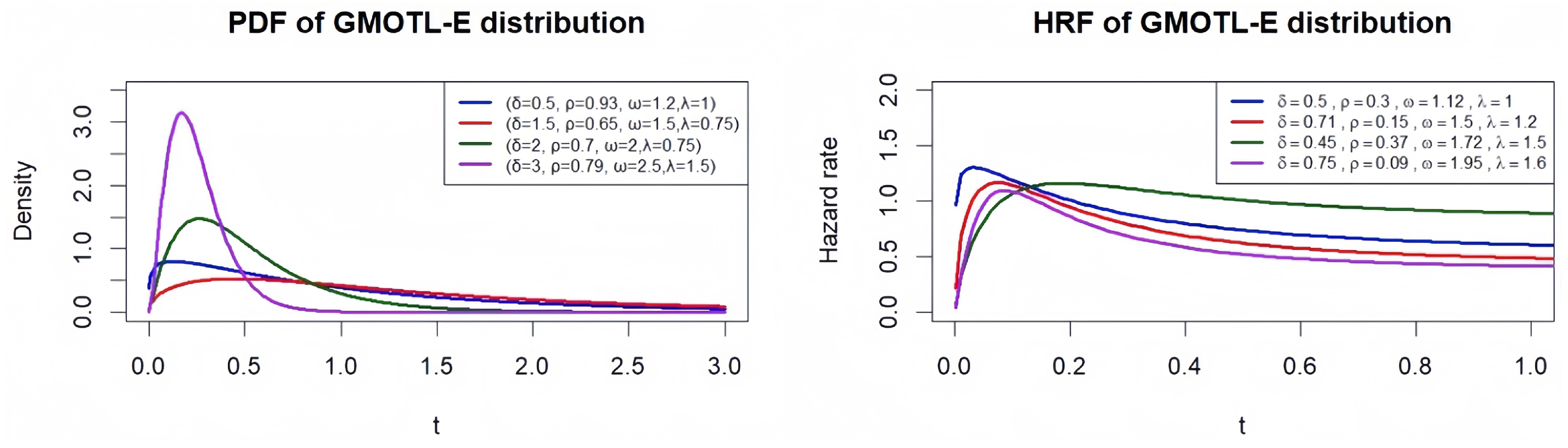
To check the shapes assumed by this distribution, we provide plots of the pdf of $GMOTL-E(\delta ,\rho ,\omega ,\lambda )$ for some parameter values (see Figure 1).

Figure 1 illustrates the shapes of the probability density function (PDF) and the hazard rate function of the GMOTL-E distribution for different parameter values. It can be observed that the proposed model is capable of capturing a wide range of behaviors.

The survival and density functions of $GMOTL-G(\delta ,\rho ,\omega )$ are expressible as a linear combination of the equivalent functions of the exponentiated $TL-G\left(\omega \right)$ distribution as outlined below. We forgo the evidence, as they are straightforward.

$$\begin{array}{ccc}\hfill S^{GMOTLG}(t;\delta ,\rho ,\omega )& =& {\rho }^{\delta }{\left\{{\overline{G}}^{TLG}(t;\omega )\right\}}^{\delta }{\displaystyle \sum _{i=0}^{\infty }}{\displaystyle \frac{(i+\delta -1)!}{(\delta -1)!i!}}{(1-\rho )}^j{\left\{{\overline{G}}^{TLG}(t;\omega )\right\}}^i\hfill \\ & =& {\displaystyle \sum _{i=0}^{\infty }}{\chi }_i^{\prime }{\left\{{\overline{G}}^{TLG}(t;\omega )\right\}}^{i+\delta }\hfill \end{array}$$

(9)

$$\begin{array}{ccc}\hfill f^{GMOTLG}(t;\delta ,\rho ,\omega )& =& -{\displaystyle \sum _{i=0}^{\infty }}{\chi }_i^{\prime }{\displaystyle \frac{d}{dt}}{\left\{{\overline{G}}^{TLG}(t;\omega )\right\}}^{i+\delta }\hfill \\ & =& g^{TLG}(t;\omega ){\displaystyle \sum _{i=0}^{\infty }}{\chi }_i{\left\{{\overline{G}}^{TLG}(t;\omega )\right\}}^{i+\delta -1}\hfill \end{array}$$

(10)

where ${\chi }_i^{\prime }={\chi }_i^{\prime }\left(\rho \right)=\left(\begin{array}{c}i+\delta -1\\ i\end{array}\right){\left(1-\rho \right)}^i{\rho }^{\delta },$ ${\chi }_i={\chi }_i\left(\rho \right)=\left(i+\delta \right){\chi }_i^{\prime }.$

$$\begin{array}{ccc}& & f^{GMOTLG}(t;\delta ,\rho ,\omega )\hfill \\ & =& {\displaystyle \sum _{i=0}^{\infty }}\left\{\begin{array}{c}{\displaystyle {\sum }_{j=0}^{i+\delta -1}}{\displaystyle {\sum }_{k=0}^{\omega (j+1)-1}}{\displaystyle {\sum }_{l=0}^{2k+1}}{\chi }_{i}2\omega {\displaystyle \frac{{(-i)}^{j+k+l}}{l+1}}\\ \times \left(\begin{array}{c}i+\delta -1\\ j\end{array}\right)\left(\begin{array}{c}\omega (j+1)-1\\ k\end{array}\right)\left(\begin{array}{c}2k+1\\ l\end{array}\right)\end{array}\right\}\left\{\left(l+1\right){g\left(t\right)G\left(t\right)}^l\right\}\hfill \\ & =& {\displaystyle \sum _{l=0}^{\infty }}\left\{\begin{array}{c}{\displaystyle {\sum }_{k=0}^{\infty }}{\displaystyle {\sum }_{j=0}^{\infty }}{\displaystyle {\sum }_{i=0}^{\infty }}{\chi }_{i}2\omega {\displaystyle \frac{{(-i)}^{j+k+l}}{l+1}}\\ \times \left(\begin{array}{c}i+\delta -1\\ j\end{array}\right)\left(\begin{array}{c}\omega (j+1)-1\\ k\end{array}\right)\left(\begin{array}{c}2k+1\\ l\end{array}\right)\end{array}\right\}\left\{\left(l+1\right){g\left(t\right)G\left(t\right)}^l\right\}\hfill \\ & =& {\displaystyle \sum _{l=0}^{\infty }}{\varpi }_l{h}_{l+1}\left(t\right)\left[since\left(\begin{array}{c}m\\ p\end{array}\right)=0,forp>m\right]\hfill \end{array}$$

(11)

where ${\varpi }_l={\sum }_{k=0}^{\infty }{\sum }_{j=0}^{\infty }{\sum }_{i=0}^{\infty }{\chi }_{i}2\omega {\displaystyle \frac{{(-i)}^{j+k+l}}{l+1}}\left(\begin{array}{c}i+\delta -1\\ j\end{array}\right)\left(\begin{array}{c}\omega (j+1)-1\\ k\end{array}\right)\left(\begin{array}{c}2k+1\\ l\end{array}\right)$ and $h_l\left(t\right)=lg\left(t\right)G{\left(t\right)}^{l-1}$ and $\left[a\right]$ means an integer part of a.

Similarly, we can write

$$F^{GMOTLG}(t;\delta ,\rho ,\omega )={\displaystyle \sum _{l=0}^{\infty }}{\varpi }_l{H}_{l+1}\left(t\right)$$

where $H_l\left(t\right)=G{\left(t\right)}^l$ is the cdf of $exp-G$ distribution with an exponentiation parameter of $(l+1)$. Some statistical characteristics of the $GMOTL-G(\delta ,\rho ,\omega )$ distributions can be derived from those of $EG$ distribution.

The proposed GMOTL-G family differs from existing extensions of the Topp–Leone-G class in several important aspects. While models such as the Marshall–Olkin TL-G, complementary geometric TL-G, Poisson TL-G by Merovci et al. (2020) [12], and odd-Weibull TL-G introduce flexibility through a single transformation mechanism, the GMOTL-G family combines the generalized Marshall–Olkin and Topp–Leone generators within a unified framework. This construction introduces two additional shape parameters, allowing for greater flexibility in modeling both the tail behavior and the hazard rate function. As a result, the proposed model provides a richer class of distributions capable of capturing more complex data patterns than existing extensions.

3. Properties of GMOTL-G

In this section, we present the main theoretical properties of the GMOTL-G family. These include the moment generating function, moments, order statistics, residual and reversed residual life functions, mean deviations, asymptotic behavior, and stochastic ordering. These results provide important insights into the structural characteristics of the proposed model and further demonstrate its flexibility and applicability in statistical modeling.

3.1. Moment Generating Function

Using Equation (8), we can express the moment generating function (mgf) in terms of the mgf of an exponentiated $TL-G\left(\omega \right)$ distribution $M_T^{E-TLG}\left(s\right)$ as follows.

$$\begin{array}{c}{M}_T^{GMOTLG}\left(s\right)=E\left[e^{sT}\right]={\int }_{-\infty }^{+\infty }{e}^{st}{f}^{GMOTLG}\left(t\right)dt=-{\int }_{-\infty }^{+\infty }{e}^{st}{\displaystyle {\sum }_{i=0}^{\infty }}{\chi }_i^{\prime }{\displaystyle \frac{d}{dt}}{\left\{{\overline{G}}^{TLG}(t;\omega )\right\}}^{i+\delta }dt\hfill \\ =-{\displaystyle {\sum }_{i=0}^{\infty }}{\chi }_i{\int }_{-\infty }^{+\infty }{e}^{st}{\displaystyle \frac{d}{dt}}{\left\{{\overline{G}}^{TLG}(t;\omega )\right\}}^{i+\delta }dt={\displaystyle {\sum }_{i=0}^{\infty }}{\chi }_i{M}_T^{E-TLG}\left(s\right)\hfill \end{array}$$

Also using Equation (9), $M_T^{GMOTLG}\left(s\right)$ can be expressed in terms of $M_{l+1}\left(s\right)$, the mgf of exponentiated-G (exp-G) with power parameter $(l+1)$, as $M_T^{GMOTLG}\left(s\right)={\sum }_{l=0}^{\infty }{\varpi }_l{M}_{l+1}\left(s\right)$. It can be written in terms of the baseline quantile function as

$$M_T^{GMOTLG}\left(s\right)={\displaystyle \sum _{l=0}^{\infty }}{\varpi }_l\tau (s,k),$$

where the quantity $\tau (s,k)={\int }_0^{1}exp\left[s{Q}_G\left(u\right)\right]u^{k}du$ can be calculated by numerical methods.

3.2. Moments in Terms of Exp-G Distribution

Let $Z_{l+1}$ be the exp-G distribution with $l+1$ power parameter. The moments of order r of T, noted as ${\mu }_r^{\prime }$, follow from Equation (9) as ${\mu }_r^{\prime }=E\left[T^r\right]={\int }_{-\infty }^{+\infty }{t}^{r}f\left(t\right)dt={\sum }_{l=0}^{\infty }{\varpi }_{l}E\left(Z_{l+1}^r\right).$

And ${\mu }_m,$ the $m^{th}$ central moment of $T,$ is:

$$\begin{array}{ccc}\hfill {\mu }_m& =& E{(T-{\mu }_1^{\prime })}^m={\displaystyle \sum _{r=0}^m}\left(\begin{array}{c}m\hfill \\ r\hfill \end{array}\right){(-{\mu }_1^{\prime })}^{m-r}E\left(T^r\right)\hfill \\ & =& {\displaystyle \sum _{r=0}^m}{\displaystyle \sum _{l=0}^{\infty }}{\varpi }_l{(-1)}^{m-r}\left(\begin{array}{c}m\hfill \\ r\hfill \end{array}\right){\left({\mu }_1^{\prime }\right)}^{m-r}E\left(Z_{l+1}^r\right)\hfill \end{array}$$

The cumulants $\left(k_n\right)$ of T follow recursively from $k_m={\mu }_m^{\prime }-{\sum }_{r=0}^{m-1}\left(\begin{array}{c}\hfill m-1\\ \hfill r-1\end{array}\right)k_r{\mu }_{m-r}^{\prime },$ where $k_1={\mu }_1^{\prime }$, $k_2={\mu }_2^{\prime }-{\mu }_1^{\prime 2}$, $k_3={\mu }_3^{\prime }-3{\mu }_2^{\prime }{\mu }_1^{\prime }-{\mu }_1^{\prime 3}$ etc.

The $s^{th}$ incomplete moment of T, say ${\Phi }_s\left(T\right)$ can be expressed from (9) as

$${\Phi }_s\left(T\right)={\int }_{-\infty }^x{t}^{s}f\left(t\right)dt={\displaystyle \sum _{l=0}^{\infty }}{\varpi }_l{\int }_{-\infty }^x{t}^s{h}_{l+1}\left(t\right)dt$$

Since closed-form expressions for the moments are not available, we provide a numerical illustration to examine the effect of the model parameters on key summary measures such as the mean, variance, and skewness.

From

Table 1. Numerical values of moments (mean, variance, and skewness) of the GMOTL-E distribution for selected parameter values.

$\mathit{\delta }$	$\mathit{\rho }$	$\mathit{\omega }$	$\mathit{\lambda }$	Mean	Variance	Skewness
0.5	1.0	1.0	1.0	1.506	1.003	1.970
1.0	1.0	1.0	1.0	1.998	1.000	2.009
1.5	1.0	1.0	1.0	2.496	0.992	1.986
1.0	0.5	1.0	1.0	1.885	0.213	0.623
1.0	1.5	1.0	1.0	2.324	4.214	4.056
1.0	1.0	0.5	1.0	1.500	0.249	2.001
1.0	1.0	1.5	1.0	2.499	2.265	2.037
1.0	1.0	1.0	0.5	2.997	3.956	1.967
1.0	1.0	1.0	1.5	1.663	0.441	2.014

, it is clear that the parameters of the $GMOTL-E$ distribution have a significant impact on the distributional characteristics. In particular, the parameter $\rho$ strongly affects the dispersion and skewness, while $\lambda$ influences the scale of the distribution. These results confirm the flexibility of the proposed model in capturing different shapes and behaviors.

3.3. Order Statistics

Suppose $T_1,T_2,\dots ,T_m$ is a random sample from the $GMOTL-G(\delta ,\rho ,\omega )$ family. Let $T_{i:m}$ be the $i^{th}$ order statistics. The pdf of $T_{i:m}$ can be expressed as

$$\begin{array}{ccc}\hfill f_{i:m}\left(t\right)& =& \frac{m!}{(i-1)!(m-i)!}{f}^{GMOTLG}\left(t\right){\left[1-{\overline{F}}^{GMOTLG}\left(t\right)\right]}^{i-1}{\left[{\overline{F}}^{GMOTLG}\left(t\right)\right]}^{m-i}\hfill \\ & =& \frac{m!}{(i-1)!(m-i)!}{f}^{GMOTLG}\left(t\right){\displaystyle \sum _{l=0}^{i-1}}{(-1)}^l\left\{{\displaystyle \frac{(i-1)!}{l!(i-l-1)!}}\right\}{\left[{\overline{F}}^{GMOTLG}\left(t\right)\right]}^{m+l-i}\hfill \end{array}$$

Using the general expansion of the $GMOTL-G(\delta ,\rho ,\omega )$ density and survival functions, we can write the pdf of the $i^{th}$ order statistics for the $GMOTL-G(\delta ,\rho ,\omega )$ family as

$$\begin{array}{ccc}\hfill f_{i:m}\left(t\right)& =& {\displaystyle \frac{m!}{(i-1)!(m-i)!}}\left\{g^{TLG}(t;\omega ){\displaystyle \sum _{e=0}^{\infty }}{\chi }_e{\left[{\overline{G}}^{TLG}\left(t;\omega \right)\right]}^{e+\delta -1}\right\}\hfill \\ & & \times {\displaystyle \sum _{l=0}^{i-1}}{(-1)}^l\left({\displaystyle \genfrac{}{}{0pt}{}{i-1}{l}}\right){\left[{\displaystyle \sum _{b=0}^{\infty }}{\chi }_b^{\prime }\left[{\overline{G}}^{TLG}{\left(t;\omega \right)}^{b+\delta }\right]\right]}^{(m+l-i)}\hfill \end{array}$$

The following is obtained by using power series for positive integer $m(\ge 1)$ (see Gradshteyn and Ryzhik, 2007) [13]:

${\left[{\sum }_{i=0}^{\infty }{a}_i{u}^i\right]}^m={\sum }_{i=0}^{\infty }{c}_{m,i}{u}^i$, where the coefficient $c_{m;i}$ for $i=1,2,\dots$ is easily obtained from the recurrence equation

$$c_{m;i}={\left(i{a}_0\right)}^{-1}{\displaystyle \sum _{p=1}^i}\left[p\left(m+1\right)-i\right]a_p{c}_{m,i-p}\mathrm{where}{c}_{m,0}=a_o^m.$$

Now

$${\left[{\displaystyle \sum _{b=0}^{\infty }}{\chi }_b^{\prime }\left[{\overline{G}}^{TLG}{\left(t;\omega \right)}^{b+\delta }\right]\right]}^{(m+l-i)}={\displaystyle \sum _{b=0}^{\infty }}{d}_{m+l-i,b+\delta }{\left[{\overline{G}}^{TLG}\left(t;\omega \right)\right]}^{b+\delta }$$

where

$$d_{m+l-i,b+\delta }={\left((b+\delta )a_0\right)}^{-1}{\displaystyle \sum _{r=1}^{b+\delta }}\left[r(m+l-i+1)-(b+\delta )\right]a_r{d}_{m+l-i;b+\delta -r}$$

Hence

$$\begin{array}{ccc}\hfill f_{i:m}\left(t\right)& =& g^{TLG}(t;\omega ){\displaystyle \sum _{e,b=0}^{\infty }}{\eta }_{e,b}{\left[{\overline{G}}^{TLG}\left(t;\omega \right)\right]}^{e+b+2\delta -1}\hfill \\ & =& -{\displaystyle \sum _{e,b=0}^{\infty }}\left[{\eta }_{e,b}/\left(e+b+2\delta \right)\right]{\displaystyle \frac{d}{dt}}{\left[{\overline{G}}^{TLG}\left(t;\omega \right)\right]}^{e+b+2\delta }\hfill \\ & =& -{\displaystyle \sum _{e,b=0}^{\infty }}{\eta }_{e,b}^{\prime }{\displaystyle \frac{d}{dt}}{\left[{\overline{G}}^{TLG}\left(t;\omega \right)\right]}^{e+b+2\delta }\hfill \end{array}$$

where ${\eta }_{e,b}=m{\chi }_e{d}_{m+l-i,b+\delta }\left({\displaystyle \genfrac{}{}{0pt}{}{m-1}{i-1}}\right){\sum }_{l=0}^{i-1}\left({\displaystyle \genfrac{}{}{0pt}{}{i-1}{l}}\right){\left(-1\right)}^l$ and ${\eta }_{e,b}^{\prime }={\eta }_{e,b}$/$\left(e+b+2\delta \right)$.

3.4. Residual Life and Reversed Residual Life

Let us consider T a random variable from $GMOTL-G(\delta ,\rho ,\omega )$ with cdf in (5). The $m^{th}$ moment of the residual life, noted as $p_m\left(x\right)=E\left[{\left(T-x\right)}^m/T>x\right]$; $m=1,2,\dots$ uniquely determines $F\left(t\right)$

$$\begin{array}{ccc}\hfill p_m\left(x\right)& =& {\displaystyle \frac{1}{1-F\left(x\right)}}{\int }_x^{\infty }{(t-x)}^{m}dF\left(t\right)={\displaystyle \frac{1}{1-F\left(x\right)}}{\int }_x^{\infty }{\displaystyle \sum _{n=0}^m}\left(\begin{array}{c}m\\ r\end{array}\right)t^r{(-x)}^{m-r}f\left(t\right)d\left(t\right)\hfill \\ & =& {\displaystyle \frac{1}{1-F\left(x\right)}}{\displaystyle \sum _{i=0}^{\infty }}{\chi }_i^{*}{\int }_x^{\infty }{t}^r{\left[{\overline{G}}^{TLG}\left(t;\omega \right)\right]}^{i+\delta -1}{g}^{TLG}(t;\omega )dt\hfill \end{array}$$

where ${\chi }_i^{*}={\chi }_i{\sum }_{r=0}^m\left(\begin{array}{c}m\\ r\end{array}\right){(-x)}^{m-r}.$

Again from Equation (9), we obtain

$$P_m\left(x\right)={\displaystyle \frac{1}{1-F\left(x\right)}}{\int }_z^{\infty }{(t-x)}^{m}dF\left(t\right)={\displaystyle \frac{1}{\overline{F}\left(x\right)}}{\displaystyle \sum _{l=0}^{\infty }}{\varpi }_l^{*}{\int }_x^{\infty }{t}^h{h}_{l+1}\left(t\right)dt,$$

where ${\varpi }_l^{*}={\varpi }_l{\sum }_{h=0}^m\left({\displaystyle \genfrac{}{}{0pt}{}{m}{h}}\right){\left(-x\right)}^{m-h}$.

For, (Mn’t), the $m^{th}$ moment of the reverse residual life, we proceed as the previous case.

$P_m\left(x\right)=E\left[{\left(x-T\right)}^m/T\le x\right]$, $x>0,m=1,2,\dots$ uniquely determines $F\left(t\right)$. We have

$$\begin{array}{ccc}\hfill P_m\left(x\right)& =& {\displaystyle \frac{1}{F\left(x\right)}}{\int }_0^x{(x-t)}^{m}dF\left(t\right)={\displaystyle \frac{1}{F\left(x\right)}}{\int }_0^x{\displaystyle \sum _{r=0}^m}{(-1)}^r\left(\begin{array}{c}m\\ r\end{array}\right)t^r{(-x)}^{m-r}f\left(t\right)d\left(t\right)\hfill \\ & =& {\displaystyle \frac{1}{F\left(x\right)}}{\displaystyle \sum _{i=0}^{\infty }}{\chi }_i^{**}{\int }_0^x{t}^r{\left[{\overline{G}}^{TLG}\left(t;\omega \right)\right]}^{i+\delta -1}{g}^{TLG}(t;\omega )dt,\hfill \end{array}$$

${\chi }_i^{**}={\chi }_i{(-1)}^m{\sum }_{r=0}^m\left(\begin{array}{c}m\\ r\end{array}\right)x^{m-r}$

Using Equation (9), it can be written as

$$P_m\left(x\right)={\displaystyle \frac{1}{F\left(x\right)}}{\int }_0^x{(x-t)}^{m}dF\left(t\right)={\displaystyle \frac{1}{F\left(x\right)}}{\displaystyle \sum _{l=0}^m}{\varpi }_l^{**}{\int }_0^x{\left(t\right)}^h{h}_{l+1}\left(t\right)dt,$$

where ${\varpi }_l^{**}={\varpi }_l{(-1)}^m{\sum }_{h=0}^m\left(\begin{array}{c}m\\ h\end{array}\right)x^{m-h}.$

3.5. Mean Deviation

Let T be the $GMOTL-G(\delta ,\rho ,\omega )$ random variable with mean $\mu =E\left(T\right)$ and median $M=Median\left(T\right)=Q\left(0.5\right)$. The mean deviations from the mean and the median can be expressed as

$${\sigma }_{\mu }\left(T\right)={\int }_{-\infty }^{\infty }\left|T-\mu \right|f\left(t\right)dt={\int }_{-\infty }^{\mu }(\mu -t)f\left(t\right)dt+{\int }_{\mu }^{+\infty }(t-\mu )f\left(t\right)dt=2\mu F\left(\mu \right)-2\Omega \left(\mu \right)$$

and

$${\sigma }_M\left(T\right)={\int }_{-\infty }^{\infty }\left|T-M\right|f\left(t\right)dt={\int }_{-\infty }^M(M-t)f\left(t\right)dt+{\int }_M^{+\infty }(t-M)f\left(t\right)dt=\mu -2\Omega \left(M\right)$$

respectively, where $F(.)$ and $f(.)$ are the cdf and pdf of the $GMOTL-G(\delta ,\rho ,\omega )$ distribution and $\Omega \left(t\right)={\int }_{-\infty }^{x}tf\left(t\right)dt.$

One can compute $\Omega \left(t\right)$ as follows: $\Omega \left(t\right)={\sum }_{i=0}^{\infty }{\chi }_i{\int }_{-\infty }^{x}t{g}^{TLG}(t;\omega ){\left[{\overline{G}}^{TLG}\left(t;\omega \right)\right]}^{i+\delta -1}dt$, where ${\chi }_i$ is as defined in Section 3.1. From Equation (9), $\Omega \left(t\right)={\int }_{-\infty }^{x}tf\left(t\right)dt.={\sum }_{l=0}^{\infty }{\varpi }_l{\int }_{-\infty }^{x}t{h}_{l+1}\left(t\right)dt$, where ${\mu }_l$ is as defined in Section 3.1.

3.6. Asymptotes

The behavior of the proposed model asymptotes are discussed here.

Proposition 1. 

The asymptotes of pdf and hrf of $GMOTL-G(\delta ,\rho ,\omega )$ are given by

$f^{GMOTLG}(t;\delta ,\rho ,\omega )⇝2\delta {\rho }^{-1}\omega g\left(t\right){(1-\overline{G}{\left(t\right)}^2)}^{\omega -1}$,                        as $t\to 0$

$f^{GMOTLG}(t;\delta ,\rho ,\omega )⇝2\delta {\rho }^{\delta }\omega g\left(t\right)\overline{G}\left(t\right){\left[1-{(1-\overline{G}{\left(t\right)}^2)}^{\omega }\right]}^{\delta -1}$,        as $t\to \infty$

$h^{GMOTLG}(t;\delta ,\rho ,\omega )⇝2\delta {\rho }^{-1}\omega g\left(t\right){(1-\overline{G}{\left(t\right)}^2)}^{\omega -1}$,                        as $t\to 0$

$h^{GMOTLG}(t;\delta ,\rho ,\omega )⇝2\delta \omega g\left(t\right)\overline{G}\left(t\right){\left[1-{(1-\overline{G}{\left(t\right)}^2)}^{\omega }\right]}^{-1}$,            as $t\to \infty$

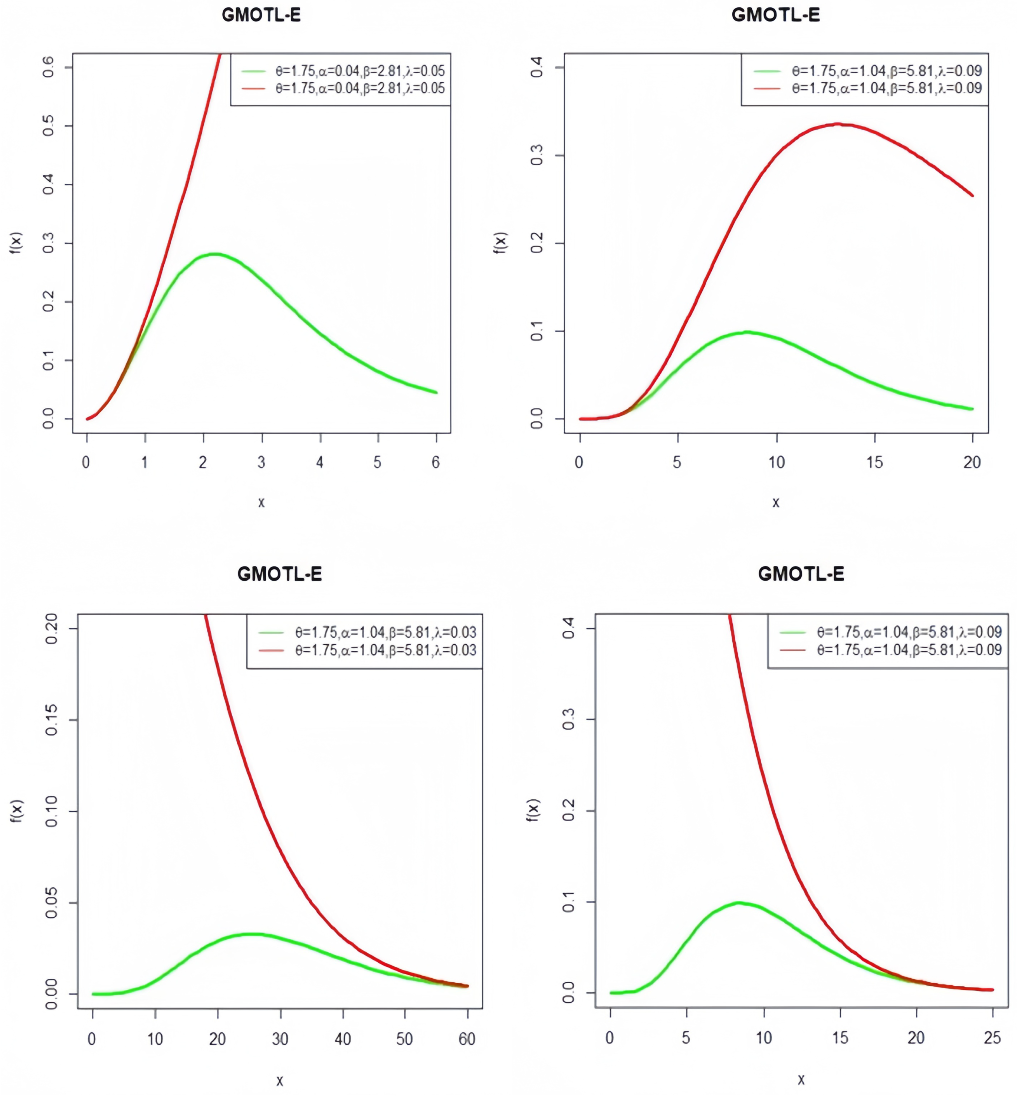
Proofs are simple and thus avoided. These results can also be checked graphically (see Figure 2) by plotting the original and corresponding asymptotic.

3.7. Stochastic Ordering

Let T and Y be two random variables with cumulative distribution functions F and G, and probability density functions f and g, respectively. Then, T is said to be smaller than Y in the likelihood ratio order (denoted by $T{\le }_{lr}Y$) if the ratio $f\left(t\right)/g\left(t\right)$ is decreasing in t, for all $t\ge 0$.

Theorem 1. 

Let $T⇝GMOTL-G(\delta ,{\rho }_1,\omega )$ and $Y⇝GMOTL-G(\delta ,{\rho }_2,\omega )$. If ${\rho }_1<{\rho }_2$, then $T{\le }_{lr}Y$. As a consequence, it follows that ($T{\le }_{hr}Y,T{\le }_{rhr}Y,T{\le }_{st}Y).$

Proof. 

Let $T⇝GMOTL-G(\delta ,{\rho }_1,\omega )$ and $Y⇝GMOTL-G(\delta ,{\rho }_2,\omega )$. If ${\rho }_1<{\rho }_2$, then

$$\begin{array}{c}{\displaystyle \frac{f\left(t\right)}{g\left(t\right)}}={\left({\displaystyle \frac{{\rho }_1}{{\rho }_2}}\right)}^{\delta }{\left[{\displaystyle \frac{1-{\overline{\rho }}_1\left[1-{(1-\overline{G}{\left(t\right)}^2)}^{\omega }\right]}{1-{\overline{\rho }}_2\left[1-{(1-\overline{G}{\left(t\right)}^2)}^{\omega }\right]}}\right]}^{\delta +1}\hfill \\ {\displaystyle \frac{d}{dt}}\left({\displaystyle \frac{f\left(t\right)}{g\left(t\right)}}\right)=(\delta +1){\left({\displaystyle \frac{{\rho }_1}{{\rho }_2}}\right)}^{\delta }({\rho }_1-{\rho }_2){\displaystyle \frac{2\omega g\left(t\right)\overline{G}\left(t\right){(1-\overline{G}{\left(t\right)}^2)}^{\omega -1}{\left(1-{\overline{\rho }}_1\left[1-{(1-\overline{G}{\left(t\right)}^2)}^{\omega }\right]\right)}^{\delta }}{{\left(1-{\overline{\rho }}_2\left[1-{(1-\overline{G}{\left(t\right)}^2)}^{\omega }\right]\right)}^{\delta +2}}}\hfill \end{array}$$

Hence, $f\left(t\right)/g\left(t\right)$ is decreasing in t. That is, $T{\le }_{lr}Y$. □

4. Parameter Estimation

In this section, we discuss parameter estimation in the case of complete as well as censored data.

4.1. Maximum Likelihood Estimation for Complete Data

To calculate the unknown parameters, we use the maximum likelihood method. Let us consider $t_1,t_{2,\dots ,}{t}_m,$ m observed values drawn from the $GMOTL-G(\delta ,\rho ,\omega )$ family with parameter vector $\Theta ={\left(\delta ,\rho ,\omega ,\zeta \right)}^T$, where $\zeta =\left({\zeta }_1,{\zeta }_2,\dots {\zeta }_q\right)$ represents the distribution parameter vector. The total log-likelihood function of $\Theta$ is given, from (5), by

$$\begin{array}{ccc}\hfill l(\Theta )& =& {\displaystyle \sum _{i=1}^m}ln\left[f\left(t_i,\Theta \right)\right]\hfill \\ & =& mln\left(2\omega \delta \right)+m\delta ln\left(\rho \right)+{\displaystyle \sum _{i=1}^m}lng(t_i,\zeta )\hfill \\ & & +{\displaystyle \sum _{i=1}^m}ln\overline{G}(t_i,\zeta )+\left(\omega -1\right){\displaystyle \sum _{i=1}^m}ln\left(1-{\overline{G}}^2(t_i,\zeta )\right)\hfill \\ & & +\left(\delta -1\right){\displaystyle \sum _{i=1}^m}ln\kappa (t_i,\zeta )-\left(\delta +1\right){\displaystyle \sum _{i=1}^m}ln\left[1-\overline{\rho }\kappa (t_i,\zeta )\right]\hfill \end{array}$$

where $\kappa (t_i,\zeta )=1-{\left[1-{\overline{G}}^2(t_i,\zeta )\right]}^{\omega }.$

By differentiating the log-likelihood function with respect to the model parameters and equating the resulting expressions to zero, we obtain the corresponding score equations. When ${\displaystyle \frac{\partial l}{\partial \delta }},{\displaystyle \frac{\partial l}{\partial \rho }},{\displaystyle \frac{\partial l}{\partial \omega }}$, and ${\displaystyle \frac{\partial l}{\partial {\zeta }_q}}$ occur simultaneously, we obtain the MLEs $\widehat{\Theta }={\left(\widehat{\delta },\widehat{\rho },\widehat{\omega },\widehat{\zeta }\right)}^T$ of $\Theta ={\left(\delta ,\rho ,\omega ,\zeta \right)}^T$. But these equations can be solved numerically using iterative methods such as the Newton–Raphson type algorithms. The score function corresponding to the parameter $\delta$ is given by

$${\displaystyle \frac{\partial \mathit{\ell }(\Theta )}{\partial \delta }}={\displaystyle \frac{m}{\delta }}+mln\left(\rho \right)+{\displaystyle \sum _{i=1}^m}ln\kappa (t_i;\zeta )-{\displaystyle \sum _{i=1}^m}ln\left[1-\overline{\rho }\kappa (t_i;\zeta )\right].$$

$${\displaystyle \frac{\partial \mathit{\ell }(\Theta )}{\partial \rho }}={\displaystyle \frac{m\delta }{\rho }}-(\delta +1){\displaystyle \sum _{i=1}^m}{\displaystyle \frac{\kappa (t_i;\zeta )}{1-\overline{\rho }\kappa (t_i;\zeta )}}.$$

$$\begin{array}{cc}\hfill {\displaystyle \frac{\partial \mathit{\ell }(\Theta )}{\partial \omega }}=& {\displaystyle \frac{m}{\omega }}+{\displaystyle \sum _{i=1}^m}ln\left(1-{\overline{G}}^2(t_i;\zeta )\right)\hfill \\ & -(\delta -1){\displaystyle \sum _{i=1}^m}{\displaystyle \frac{{\overline{G}}^{\omega }(t_i;\zeta )ln\overline{G}(t_i;\zeta )}{\kappa (t_i;\zeta )}}\hfill \\ & +(\delta +1)\overline{\rho }{\displaystyle \sum _{i=1}^m}{\displaystyle \frac{{\overline{G}}^{\omega }(t_i;\zeta )ln\overline{G}(t_i;\zeta )}{1-\overline{\rho }\kappa (t_i;\zeta )}}.\hfill \end{array}$$

Finally, the score function with respect to the baseline parameter $\zeta$ is given in the general form

$$\begin{array}{cc}\hfill {\displaystyle \frac{\partial \mathit{\ell }(\Theta )}{\partial \zeta }}=& {\displaystyle \sum _{i=1}^m}{\displaystyle \frac{\partial }{\partial \zeta }}lng(t_i;\zeta )+{\displaystyle \sum _{i=1}^m}{\displaystyle \frac{\partial }{\partial \zeta }}ln\overline{G}(t_i;\zeta )\hfill \\ & +(\omega -1){\displaystyle \sum _{i=1}^m}{\displaystyle \frac{\partial }{\partial \zeta }}ln\left(1-{\overline{G}}^2(t_i;\zeta )\right)\hfill \\ & +(\delta -1){\displaystyle \sum _{i=1}^m}{\displaystyle \frac{\partial }{\partial \zeta }}ln\kappa (t_i;\zeta )-(\delta +1){\displaystyle \sum _{i=1}^m}{\displaystyle \frac{\partial }{\partial \zeta }}ln\left[1-\overline{\rho }\kappa (t_i;\zeta )\right].\hfill \end{array}$$

4.2. Maximum Likelihood Estimation for Right-Censored Data

In this paper, we assume independent random right censoring, where the lifetime variables are $T_1,T_{2,\dots ,}{T}_m$ from the $GMOTL-G(\delta ,\rho ,\omega )$ distribution. In this case, each observation can be written as $t_i=min\left(T_i,C_i\right)$ for $i=1,\dots ,n$, where $T_i$ and C are respectively the failure and censoring times. We presume that the censoring times are independent of the parameters; hence, the probability function can be expressed as

$$L(t,\Theta )={\displaystyle \prod _{i=1}^m}{f}^{{\Delta }_i}\left(t_i\right)S^{1-{\Delta }_i}\left(t_i\right),{\Delta }_i=1_{\left\{T_i<C_i\right\}}$$

Then

$$\begin{array}{ccc}\hfill I_m(t,\Theta )& =& {\displaystyle \sum _{i=1}^m}{\Delta }_{i}ln\left[f\left(t_i\right)\right]+{\displaystyle \sum _{i=1}^m}(1-{\Delta }_i)lnS\left(t_i\right)\hfill \\ & =& {\displaystyle \sum _{i=1}^m}{\Delta }_i\left[\begin{array}{c}ln\left(2\delta \omega \right)+\delta ln\left(\rho \right)+lng(t_i,\zeta )+ln\overline{G}(t_i,\zeta )\\ +(\omega -1)ln\left[1-{\overline{G}}^2(t_i,\zeta )\right]+\left(\delta -1\right)ln\kappa (t_i,\zeta )\\ -(\delta +1)ln\left[1-\overline{\rho }\kappa \left(t_i,\zeta \right)\right]\end{array}\right]\hfill \\ & & +\delta {\displaystyle \sum _{i=1}^m}(1-{\Delta }_i)ln\left[{\displaystyle \frac{\rho \kappa (t_i,\zeta )}{1-\overline{\rho }\kappa \left(t_i,\zeta \right)}}\right]\hfill \end{array}$$

The maximum likelihood estimators are obtained by differentiating the log-likelihood function with respect to the parameters and equating the resulting expressions to zero, which yields a system of score equations. Due to the complexity of these equations, numerical methods are employed to obtain the estimates.

5. Goodness-of-Fit Testing Under Right Censoring

In this section, we develop a goodness-of-fit testing procedure for the proposed model under independent right censoring. The test is constructed based on a chi-square type approach and is adapted to the GMOTL-E distribution. This section constitutes one of the main contributions of the paper, as it provides a practical tool for assessing model adequacy when censored observations are present.

5.1. Framework Under Right Censoring

Let $T_1,T_2,\dots ,T_m$ be independent and identically distributed random variables representing the lifetimes of interest, and let $C_1,C_2,\dots ,C_m$ be independent censoring times. Instead of observing $T_i$ directly, we observe $t_i=min(T_i,C_i)$ together with the censoring indicators.

We assume that the censoring mechanism is independent of the lifetime distribution, which corresponds to the standard independent right-censoring scheme commonly used in survival analysis and reliability studies.

5.2. Construction of the Test Statistic

In the situation where the complete data case is available, different goodness-of-fit tests are developed in the statistical literature, but for censored data, this is not the case. Here and using the method of Bagdonavicius and Nikulin (2011) [14], we constructed a new test statistic for $GMOTL-G(\delta ,\rho ,\omega )$ distribution for right-censored data Given m i.i.d. random variable $T_1,T_2,\dots ,T_m$ following a parametric model $F_0$, our aim is to test the hypothesis that the sampled data come from the distribution $F_0(t;\xi ),$ $t\ge 0,$ $\Theta ={({\Theta }_1,{\Theta }_{2,}\dots {\Theta }_s)}^T,$$\Theta \subset R^s.$

$$\mathrm{That} \mathrm{is}, H_0:P(T_i\le t\mid H_0)=F_0(t;\Theta ), t\ge 0 \mathrm{and} \Theta ={({\Theta }_1,{\Theta }_{2,}\dots {\Theta }_s)}^T,$$

These observations are grouped into r classes $I_j$, for $j=1,2,\dots ,r$. We propose a test statistic $Y^2$ for right censoring with unknown parameters. This test statistic $Y^2$ is defined by

$$Y^2={\displaystyle \sum _{j=1}^r}{\displaystyle \frac{{(U_j-e_j)}^2}{U_j}}+Q$$

$U_j,$ $e_j$ represent the observed and the expected number of T in the intervals $I_j$, and Q is a quadratic from given as $Q=W^T{\widehat{D}}^{-}W,where$ $W={\left(W_1,W_2,\dots W_s\right)}^T,$ ${\widehat{W}}_l={\sum }_{j=1}^r{\widehat{C}}_{lj}{\widehat{A}}_j^{-1}{Z}_j,$

${\widehat{C}}_{lj}={\displaystyle \frac{1}{m}}{\sum }_{i:t_i\in I_j}{\delta }_i{\displaystyle \frac{\partial lnh(t_i,\widehat{\Theta })}{\partial \Theta }},$   ${\widehat{A}}_j=U_j/m,$   $U_j={\sum }_{i:T_i\in I_j}{\Delta }_i,$

$\widehat{D}={\left[{\widehat{d}}_{l{l}^{\prime }}\right]}_{s\times s}$,   ${\widehat{d}}_{l{l}^{\prime }}={\widehat{i}}_{l{l}^{\prime }}-{\sum }_{j=1}^r{\widehat{C}}_{lj}{\widehat{C}}_{l^{\prime }j}{\widehat{A}}_j^{-1},$  $l,l^{\prime }=1,\dots ,s,$

$Z_j={\displaystyle \frac{1}{\sqrt{m}}}\left(U_j-e_j\right),$   $j=1,2,\dots ,r$

and ${\widehat{i}}_{l{l}^{\prime }}={\displaystyle \frac{1}{m}}{\sum }_{i=1}^m{\delta }_i{\displaystyle \frac{\partial lnh(t_i,\widehat{\Theta })}{\partial {\Theta }_l}}{\displaystyle \frac{\partial lnh(t_i,\widehat{\Theta })}{\partial {\Theta }_{l^{\prime }}}}.$

Under the null hypothesis is $H_0$; this statistic $Y^2$ follows a chi-square distribution. This approach is commonly used in the statistical literature to construct goodness-of-fit tests for a wide range of models, including those based on Bertholon-type formulations, generalized exponential AFT structures, and AFT-generalized inverse Weibull distributions.

5.3. Goodness-of-Fit Test for GMOTL-E Distribution

We examine a right-censored sample from $GMOTL-E\left(\delta ,\rho ,\omega ,\lambda \right).$ As previously said, $t_i$ represents the minimum value between $T_i$ and $C_i$. Let $\tau$ be a finite duration, during which we categorized the observed data into $r>4$ sub-intervals $I_j=(a_{j-1}-a_j)$ of $\left[0,\tau \right]$. To verify $H_0$ that this sample originates from the $GMOTL-E\left(\delta ,\rho ,\omega ,\lambda \right)$ distribution, we must first estimate the interval bounds $a_j$, which are provided by

$${\widehat{a}}_j=H^{-1}\left({\displaystyle \frac{E_j-{\sum }_{l=1}^{i-1}H\left(t_l,\widehat{\Theta }\right)}{m-i+1}},\widehat{\Theta }\right),{\widehat{a}}_r=max\left(T_{\left(m\right),}\tau \right)$$

$H\left(t_l,\widehat{\Theta }\right)$ is the cumulative hazard rate function of $GMOTL-E$ and $\widehat{\Theta }$ is the maximum likelihood parameter estimators for initial data. We then obtain the values of $U_j$ and $e_j$ $\left(e_j={\displaystyle \frac{E_r}{r}}\mathrm{for}\mathrm{any}j,\mathrm{with}{E}_r={\sum }_{i=1}^{m}H\left(t_i,\widehat{\Theta }\right)\right)$.

So, we have

$$E_j={\displaystyle \frac{-j\delta }{k-1}}{\displaystyle \sum _{i=1}^m}ln\left({\displaystyle \frac{\rho \left\{1-{\left(1-e^{-2\lambda t_i}\right)}^{\omega }\right\}}{1-\overline{\rho }\left\{1-{\left(1-e^{-2\lambda t_i}\right)}^{\omega }\right\}}}\right),j=1,\dots r-1$$

we note ${\xi }_i=1-{\left(1-e^{-2\lambda t_i}\right)}^{\omega }$.

Computation of the Quadratic Form Q

For our model, the elements of $\widehat{C}$ are given as follows

$${\widehat{C}}_{lj}={\displaystyle \frac{1}{m}}{\displaystyle \sum _{i:t_i\in I_j}^m}{\Delta }_i{\displaystyle \frac{\partial }{\partial {\widehat{\Theta }}_l}}lnh(t_i;\widehat{\Theta })\mathrm{where}$$

$$lnh\left(t_i\right)=ln\left(2\delta \rho \omega \right)+\delta ln\rho -2\lambda t_i+(\omega -1)ln(1-e^{-2\lambda t_i})-ln\left({\xi }_i\right)-ln(1-\overline{\rho }{\xi }_i)$$

are obtained as below

$${\widehat{C}}_{1j}={\displaystyle \sum _{i:t_i\in I_j}^m}{\Delta }_i\left({\displaystyle \frac{\delta }{\rho }}-{\displaystyle \frac{{\xi }_i}{1-\overline{\rho }{\xi }_i}}\right)$$

$${\widehat{C}}_{2j}={\displaystyle \sum _{i:t_i\in I_j}^m}{\Delta }_i\left({\displaystyle \frac{1}{\lambda }}-2t_i+\frac{2(\omega -1)t_i{e}^{-2\lambda t_i}}{1-e^{-2\lambda t_i}}+\frac{2\omega t_i{e}^{-2\lambda t_i}{\left(1-e^{-2\lambda t_i}\right)}^{\omega -1}}{1-{\left(1-e^{-2\lambda t_i}\right)}^{\omega }}-\frac{2\overline{\rho }\omega t_i{e}^{-2\lambda t_i}{\left(1-e^{-2\lambda t_i}\right)}^{\omega -1}}{1-\overline{\rho }{\xi }_i}\right)$$

$${\widehat{C}}_{3j}={\displaystyle \sum _{i:t_i\in I_j}^m}{\Delta }_i\left({\displaystyle \frac{1}{\omega }}+ln\left(1-e^{-2\lambda t_i}\right)+\frac{{\left(1-e^{-2\lambda t_i}\right)}^{\omega }ln\left(1-e^{-2\lambda t_i}\right)}{1-{\left(1-e^{-2\lambda t_i}\right)}^{\omega }}-\frac{\overline{\rho }{\left(1-e^{-2\lambda t_i}\right)}^{\omega }ln\left(1-e^{-2\lambda t_i}\right)}{1-\overline{\rho }{\xi }_i}\right)$$

$${\widehat{C}}_{4j}={\displaystyle \sum _{i:t_i\in I_j}^m}{\Delta }_i\left({\displaystyle \frac{1}{\delta }}+ln\left(\rho \right)\right)$$

Therefore, the statistic $Y_m^2$ can be easily computed for the $GMOTL-E\left(\delta ,\rho ,\omega ,\lambda \right)$ distribution in the case of right censorship and unknown parameters. This statistic is distributed as a chi-square with r degrees of freedom.

$$Y_m^2\left(\widehat{\Theta }\right)={\displaystyle \sum _{j=1}^r}{\displaystyle \frac{{\left(U_j-e_j\right)}^2}{U_j}}+{\widehat{W}}^T{\left[{\widehat{ı}}_{l{l}^{\prime }}-{\displaystyle \sum _{j=1}^r}{\widehat{C}}_{lj}{\widehat{C}}_{l^{\prime }j}{\widehat{A}}_j^{-1}\right]}^{-1}\widehat{W}$$

6. Simulations

In this section, we investigate the finite-sample performance of the maximum likelihood estimators and the proposed goodness-of-fit test for the GMOTL-E distribution.

6.1. Simulation Setup

Random samples were generated from the GMOTL-E distribution for different combinations of the parameters $\delta ,\rho ,\omega ,\lambda$. The following parameter configurations were considered:

$$(2,1.5,0.7,2),(0.5,1,1.6,1.2),(1.5,0.7,1,0.8)$$

For each configuration, samples of sizes $n=10,20,45,120,300$ were generated. Each experiment was replicated $M=1000$ times to ensure stable results.

The performance of the maximum likelihood estimators was evaluated using the bias and mean square error (MSE), defined as:

$$\mathrm{MSE}\left(\widehat{\theta }\right)=\mathbb{E}\left[{(\widehat{\theta }-\theta )}^2\right].$$

6.2. Results for Parameter Estimation

The results of the simulation study are summarized in

Table 2. Simulation results for different parameter configurations and sample sizes.

m	$\mathit{\delta }=2$	$\mathit{\rho }=1.5$	$\mathit{\omega }=0.7$	$\mathit{\lambda }=2$
10	1.9643 (0.0067)	1.4684 (0.0079)	0.7249 (0.0089)	2.0229 (0.0063)
20	1.9729 (0.0052)	1.4768 (0.0064)	0.7153 (0.0072)	2.0193 (0.0049)
45	1.9785 (0.0046)	1.4809 (0.0053)	0.7126 (0.0059)	2.0157 (0.0037)
120	1.9873 (0.0028)	1.4865 (0.0032)	0.7097 (0.0038)	2.0092 (0.0025)
300	1.9983 (0.0012)	1.4962 (0.0019)	0.7014 (0.0022)	2.0012 (0.0013)
$\mathit{m}$	$\mathit{\delta }=\mathbf{0}.\mathbf{5}$	$\mathit{\rho }=\mathbf{1}$	$\mathit{\omega }=\mathbf{1}.\mathbf{6}$	$\mathit{\lambda }=\mathbf{1}.\mathbf{2}$
10	0.4757 (0.0098)	0.8731 (0.0078)	1.6281 (0.0066)	1.0736 (0.0073)
20	0.4791 (0.0083)	0.8809 (0.0060)	1.6196 (0.0053)	1.0814 (0.0056)
45	0.4856 (0.0071)	0.9779 (0.0042)	1.6156 (0.0036)	1.1784 (0.0039)
120	0.4902 (0.0049)	0.9884 (0.0028)	1.6085 (0.0020)	1.1889 (0.0023)
300	0.4987 (0.0015)	0.9973 (0.0019)	1.6051 (0.0006)	1.1978 (0.0007)
$\mathit{m}$	$\mathit{\delta }=\mathbf{1}.\mathbf{5}$	$\mathit{\rho }=\mathbf{0}.\mathbf{7}$	$\mathit{\omega }=\mathbf{1}$	$\mathit{\lambda }=\mathbf{0}.\mathbf{8}$
10	1.5278 (0.0045)	0.7197 (0.0062)	0.9745 (0.0077)	0.7758 (0.0056)
20	1.5216 (0.0033)	0.7135 (0.0050)	0.9835 (0.0061)	0.7843 (0.0043)
45	1.5167 (0.0024)	0.7086 (0.0031)	0.9886 (0.0048)	0.7899 (0.0036)
120	1.5121 (0.0016)	0.7042 (0.0023)	0.9942 (0.0031)	0.7955 (0.0019)
300	1.5089 (0.0009)	0.7008 (0.0016)	0.9985 (0.0018)	0.7998 (0.0006)

, which reports the estimated values, bias, and mean square error for different parameter configurations and sample sizes.

From Table 2, it is observed that the performance of the maximum likelihood estimators improves as the sample size increases. In particular, both the bias and the mean square error decrease with increasing sample size, indicating the consistency of the estimators.

Moreover, the estimators remain stable across different parameter configurations, which confirms the robustness of the estimation procedure.

6.3. Comparison Between Complete and Right-Censored Samples

To evaluate the impact of censoring on the efficiency of the estimators, we compare the maximum likelihood estimates obtained from complete samples with those obtained from right-censored samples under the same parameter configurations.

Right-censored samples were generated under the assumption of independent censoring. Two censoring levels, namely 20% and 40%, were considered to examine how increasing censoring proportions affect the estimation accuracy.

The same simulation setup described previously was used for both complete and censored samples.

From

Table 3. Comparison of parameter estimation under complete and right-censored samples.

Data Type	n	Censoring	$\mathit{\delta }=2$	$\mathit{\rho }=1.5$	$\mathit{\omega }=0.7$	$\mathit{\lambda }=2$
n = 20, 45
Complete	20	0	2.008 (0.0038)	1.507 (0.0047)	0.687 (0.0058)	1.985 (0.0041)
Censored	20	20 %	1.972 (0.0052)	1.476 (0.0064)	0.715 (0.0072)	2.019 (0.0049)
Censored	20	40 %	1.981 (0.0063)	1.482 (0.0073)	0.720 (0.0078)	2.021 (0.0056)
Complete	45	0	2.006 (0.0022)	1.505 (0.0030)	0.690 (0.0043)	1.987 (0.0032)
Censored	45	20 %	1.978 (0.0046)	1.480 (0.0053)	0.712 (0.0059)	2.0157 (0.0037)
Censored	45	40 %	1.984 (0.0039)	1.485 (0.0059)	0.718 (0.0064)	2.018 (0.0045)
n = 120, 300
Complete	120	0	2.004 (0.0013)	1.503 (0.0021)	0.695 (0.0014)	1.990 (0.0016)
Censored	120	20 %	1.987 (0.0028)	1.486 (0.0032)	0.709 (0.0038)	2.009 (0.0025)
Censored	120	40 %	1.985 (0.0032)	1.486 (0.0034)	0.714 (0.0042)	2.015 (0.0030)
Complete	300	0	2.002 (0.0007)	1.501 (0.0012)	0.699 (0.0008)	1.992 (0.0009)
Censored	300	20 %	1.998 (0.0012)	1.496 (0.0019)	0.701 (0.0022)	2.001 (0.0013)
Censored	300	40 %	1.986 (0.0020)	1.489 (0.0023)	0.712 (0.0032)	2.013 (0.0027)

, it is observed that the estimators obtained from complete data generally have smaller biases and mean square errors compared to those obtained from right-censored data.

As the censoring proportion increases, the estimation accuracy decreases, which is expected due to the loss of information caused by censoring. This effect is more pronounced for smaller sample sizes.

However, the estimators remain reasonably stable even under moderate levels of censoring, and the overall performance improves as the sample size increases. These results indicate that the proposed estimation procedure is robust and performs satisfactorily in the presence of right censoring.

6.4. Test Statistic $Y^2$

To check the validity of the hypothesis—that is, $H_0$—that the right-censored sample belongs to the $GMOTL-E\left(\delta ,\rho ,\omega ,\lambda \right)$ model, we compute the statistic criteria $Y_n^2\left(\widehat{\Theta }\right)$ for the generated samples. The empirical levels of significance, $Y^2>{\chi }_{\epsilon }^2\left(r\right)$, corresponding to theoretical levels of significance $(\epsilon =0.10,0.05,0.01)$, obtained are given in

Table 4. Simulated levels of significance for $Y_n^2(\Theta )$ test for GMOTL-E model against their theoretical values ($\epsilon$ 0.01, 0.05, 0.10).

M	$\mathit{m}=10$	$\mathit{m}=20$	$\mathit{m}=45$	$\mathit{m}=120$	$\mathit{m}=300$
$\epsilon =1\%$	$0.0052$	$0.0065$	$0.0075$	$0.0087$	$0.0096$
$\epsilon =5\%$	$0.0449$	$0.0456$	$0.0463$	$0.0476$	$0.0482$
$\epsilon =10\%$	$0.0951$	$0.0963$	$0.0974$	$0.0989$	$0.0994$

. We have chosen $r=5$ classes to group the data.

Regarding these results, we can say that the simulated samples are fitted by distribution for the different levels of significance, which confirms the applicability of the proposed test in this work. Therefore, the same can be safely used to validate data fitting from this new distribution.

7. Real Data Modeling

7.1. Comparative Assessment of $GMOTL-E$ in Modeling Uncensored Data

Below displays

Table 5. Descriptive statistics for Sierra Leone COVID-19 daily reported new cases.

Datasets	m	Min	Mean	Median	S.d	Skewness	Kurtosis	Max
I	64	1	$19.77$	7	$29.59$	$2.5$	$10.51$	160

the daily reported new COVID-19 cases in Sierra Leone [2]. The dataset covers several days of reported cases, illustrating fluctuations in the number of new infections. The values represent the daily counts of new cases over a certain period.

$$3,15,1,1,1,11,18,19,34,5,15,48,86,160,72,92,81,50,65,41,48,40,44,30,23,43,6,7,32,$$

$$7,13,16,13,2,14,4,5,5,12,6,3,14,1,3,1,3,7,1,2,2,1,9,1,10,2,2,7,2,1,1,1,1,1,1.$$

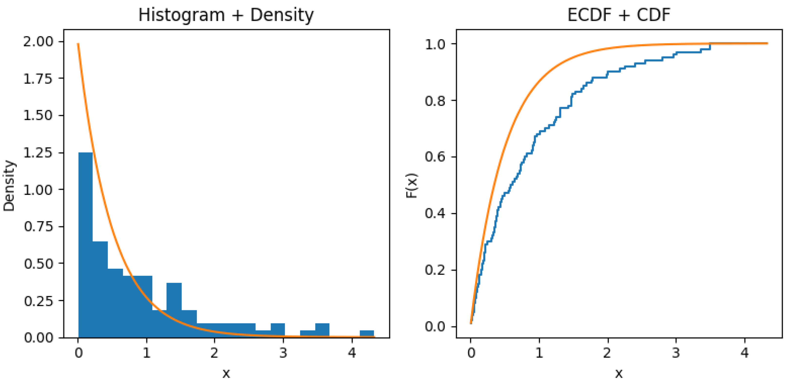
To further assess the goodness-of-fit of the proposed model [15], we provide graphical comparisons based on both the density and distribution functions as shown in Figure 3.

As shown in the figure, the GMOTL-E model provides a reasonable fit to the data in both the density and distribution representations, which supports the numerical goodness-of-fit results.

This study demonstrates that the $GMOTL-E\left(\delta ,\rho ,\omega ,\lambda \right)$ distributions from the proposed family are formidable competitors to the Marshall–Olkin Kumaraswamy exponential (MOKw-E), Kumaraswamy Marshall–Olkin exponential (KwMO-E) (Alizadeh et al., 2015 [16]), Beta Poisson exponential, Kumaraswamy Poisson exponential (KwP-E) (Chakraborty et al., 2020 [11]), and Marshall Olkin Topp–Leone exponential (Handique et al., 2020 [11]) distributions. We have evaluated various classical model selection criteria to compare the fitted models. We have also supplied the maximum likelihood estimates (MLEs) of the parameters together with their standard errors for the alternatives. The results presented in

Table 6. MLEs nd their standard errors (in parentheses) for the guinea pig survival times dataset.

Distributions	$\widehat{\mathit{\delta }}$	$\widehat{\mathit{\rho }}$	$\widehat{\mathit{a}}$	$\widehat{\mathit{\omega }}$	$\widehat{\mathit{\lambda }}$
$MOKw-E\left(\rho ,a,\omega ,\lambda \right)$	−	0.0051 0.0018	3.0512 0.0085	2.2451 0.0043	0.0647 0.0053
$KwMO-E\left(a,\omega ,\rho ,\lambda \right)$	−	0.6478 0.0856	3.6125 0.0794	2.9562 0.0912	0.4612 0.8451
$BP-E\left(a,\omega ,\delta ,\lambda \right)$	0.028 0.034	−	2.9874 0.7632	0.6786 1.2365	1.8459 0.7235
$KwP-E\left(a,\omega ,\delta ,\lambda \right)$	3.162 2.631	−	2.9452 0.0862	3.1845 0.7624	0.2347 0.1374
$MOTL-E\left(\rho ,\omega ,\lambda \right)$	−	0.4982 0.3743	−	4.2657 0.5321	0.4963 0.1267
$GMOTL-E\left(\delta ,\rho ,\omega ,\lambda \right)$	2.378 0.731	0.1024 0.0785	−	1.9823 0.5264	0.0794 0.2137

and

Table 7. AIC, BIC, CAIC, HQIC, A, W and KS (p-value) values for the guinea pig survival times dataset.

Distributions	$\mathit{AIC}$	$\mathit{BIC}$	$\mathit{CAIC}$	$\mathit{HQIC}$	A	W	$\mathit{KS}$ (p-Value)
$MOKw-E\left(\rho ,a,\omega ,\lambda \right)$	$114.11$	$123.23$	$114.71$	$117.71$	$0.71$	$0.09$	$0.020\left(0.90\right)$
$KwMO-E\left(a,\omega ,\rho ,\lambda \right)$	$112.47$	$121.61$	$113.09$	$116.09$	$0.53$	$0.08$	$0.019\left(0.91\right)$
$BP-E\left(a,\omega ,\delta ,\lambda \right)$	$110.09$	$119.17$	$110.69$	$113.69$	$0.40$	$0.04$	$0.017\left(0.93\right)$
$KwP-E\left(a,\omega ,\delta ,\lambda \right)$	$111.30$	$120.41$	$111.90$	$114.93$	$0.47$	$0.05$	$0.018\left(0.92\right)$
$MOTL-E\left(\rho ,\omega ,\lambda \right)$	$109.39$	$116.22$	$109.74$	$112.11$	$0.36$	$0.03$	$0.016\left(0.94\right)$
$GMOTL-E\left(\delta ,\rho ,\omega ,\lambda \right)$	$105.79$	$114.87$	$106.38$	$109.39$	$0.28$	$0.02$	$0.015\left(0.95\right)$

unequivocally demonstrate the superiority of the proposed model compared to the alternatives across all criteria. Although all distributions were thoroughly surpassed by the suggested model, we have only shown the findings for four-parameter models here.

The top-performing models, namely $MOTL-E$ and $GMOTL-E$, offer greater flexibility due to their incorporation of shape parameters such as $\delta$ and $\rho$. This flexibility facilitates improved modeling of asymmetry and heavy tails in the data. As a result, these models provide a more accurate representation of the underlying distribution, ultimately enhancing predictive performance. Consequently, they are better suited for applications involving data that display significant deviations from normality.

The $GMOTL-E$ distribution clearly outperforms all others across all model selection criteria:

• It has the lowest values for $AIC$, $BIC$, $CAIC$, and $HQIC$, indicating an optimal trade-off between model fit and complexity.
• The best goodness-of-fit statistics (lowest A, W, and $KS$ values), with a $KS$ p-value of $0.95$, suggest excellent agreement between the empirical and theoretical distributions.

$MOTL-E$ is the second-best performer but slightly less accurate than $GMOTL-E$, showing the added value of the $\delta$ parameter in $GMOTL-E$. This distinction emphasizes the value of incorporating additional parameters to enhance model precision. Additionally, the better performance of $GMOTL-E$ indicates that improving its design could lead to even stronger prediction abilities in future uses.

Traditional models like $BP-E$ or $MOKw-E$ perform significantly worse, supporting the relevance and strength of the proposed new distributional family.

7.2. Right-Censored Data Analysis with GMOTL-E

To illustrate the adaptability of our model, we utilize actual, censored data representing the duration (in months) from diagnosis to death for 31 patients displaying advanced non-Hodgkin’s lymphoma clinical symptoms, as reported by Gijbels and Gurler (2003) [17], who applied an exponential change point model to characterize this data. Eleven of the thirty-one observations are censored, as the patients remained alive at the final follow-up.

2.5, 4.1, 4.6, 6.4, 6.7, 7.4, 7.6, 7.7, 7.8, 8.8, 13.3, 13.4, 18.3, 19.7, 21.9, 24.7, 27.5, 29.7, 30.1 *, 32.9, 33.5, 35.4 *, 37.7 *, 40.9 *, 42.6, 45.4, 48.5 *, 48.9 *, 60.4, 64.4 *, 66.4 *.

The asterisk (*) indicates a suppressed observation.

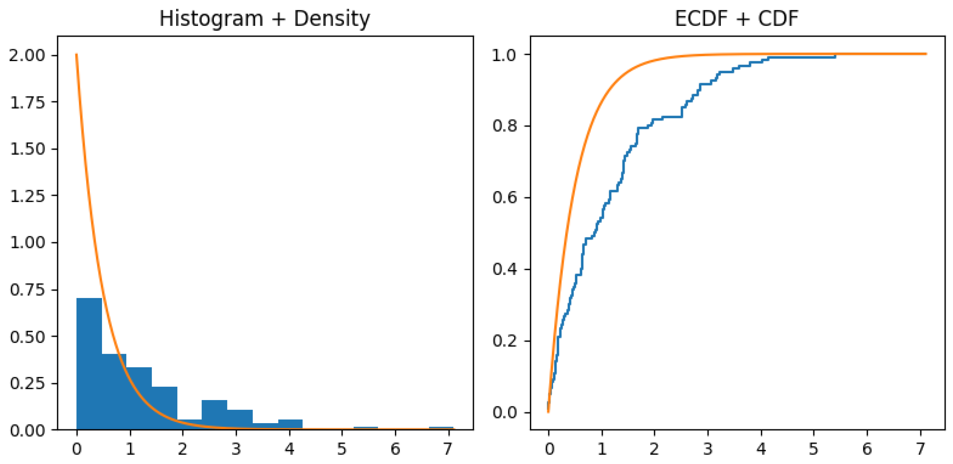
To further assess the goodness-of-fit of the proposed model for the second dataset, we provide graphical comparisons based on both the density and distribution functions as shown in Figure 4.

As shown in the figure, the GMOTL-E model provides a satisfactory fit to the second dataset in both the density and distribution representations, which supports the goodness-of-fit results obtained earlier.

We employ the aforementioned statistical test to ascertain whether these data conform to the $GMOTL-E\left(\delta ,\rho ,\omega ,\lambda \right)$ distribution. We will initially estimate the parameters of the GMOTL-E distribution using the available uncensored observations while effectively addressing the filtered data. Subsequently, we can do goodness-of-fit tests to assess the model’s appropriateness for the dataset, ensuring that the conclusions are robust and reliable. We initially calculate the maximum likelihood estimators of the unknown parameters as

$$\widehat{\Theta }={\left(\widehat{\rho },\widehat{\lambda },\widehat{\omega },\widehat{\delta }\right)}^T={\left(1.1063,0.8921,1.8263,3.9467\right)}^T.$$

The data are subsequently categorized into $r=6$ intervals $I_j$. The requisite calculations are shown in

Table 8. Values of ${\widehat{a}}_j,e_j,U_j,{\widehat{C}}_{1j},{\widehat{C}}_{2j},{\widehat{C}}_{3j},{\widehat{C}}_{4j}$.

${\widehat{\mathit{a}}}_{\mathit{j}}$	$7.2$	$15.8$	$29.9$	$36.8$	$46.8$	$66.4$
$U_J$	5	7	6	4	4	5
${\widehat{C}}_{1j}$	$-0.9562$	$-1.0856$	$-4.2563$	$-7.5236$	$-0.7182$	$-1.866$
${\widehat{C}}_{2j}$	$1.8965$	$2.5138$	$1.9856$	$0.8956$	$0.7154$	$0.6235$
${\widehat{C}}_{3j}$	$1.0265$	$1.5845$	$1.1263$	$0.9563$	$0.7152$	$0.6945$
${\widehat{C}}_{4j}$	$1.7791$	$2.4807$	$2.1263$	$0.7087$	$0.7087$	$0.3543$
$e_j$	$1.3259$	$1.3259$	$1.3259$	$1.3259$	$1.3259$	$1.3259$

.

Then, we obtain the value of the statistic test $Y_n^2$ as:

$$Y_m^2={\displaystyle \sum _{j=1}^r}{\displaystyle \frac{{(U_j-e_j)}^2}{U_j}}+Q=4.9562+4.8236=9.7798$$

For significance level $\epsilon =0.05$, the critical value ${\chi }_6^2=12,5916$ is higher than the value of $Y_m^2=9.7798,$ so we can say that the proposed $GMOTL-E$ model fits these data.

8. Conclusions

In this paper, we introduced a new extension of the Topp–Leone-G family, called the generalized Marshall–Olkin Topp–Leone-G (GMOTL-G) family of distributions. The proposed family was constructed by combining the generalized Marshall–Olkin and Topp–Leone-G generators in order to obtain a more flexible class of models for lifetime data. We showed that this family contains important existing models as special cases and offers greater flexibility for modeling different distributional behaviors.

We pay particular attention to the generalized Marshall-Olkin Topp-Leone exponential distribution (GMOTL-E) as a useful special case of the proposed family. Several of its mathematical and statistical properties were derived and discussed, including moments, order statistics, residual life and reversed residual life functions, mean deviations, asymptotic behavior, and stochastic ordering. The analytical developments, together with the graphical illustrations, show that the proposed model is capable of capturing different shapes of the density and hazard rate functions, which makes it attractive for practical applications.

From an inferential point of view, we developed maximum likelihood estimation for the model parameters with both complete and right-censored data. We also constructed a goodness-of-fit test for the proposed model under independent right censoring using a chi-square type approach. The simulation study showed that the maximum likelihood estimators behave well, with mean square errors decreasing as the sample size increases, and that the proposed test provides empirical significance levels that are close to the corresponding theoretical levels. These results support the usefulness of the estimation and testing procedures developed in this work. The practical performance of the proposed model was illustrated through two real-data applications. In the uncensored data analysis, the GMOTL-E model provided the best fit among the competing models considered, according to the model selection criteria and goodness-of-fit measures. In the right-censored application, the proposed goodness-of-fit test indicated that the GMOTL-E model gives an adequate fit to the data. These findings show that the new family is not only mathematically interesting, but also useful in real modeling situations involving both complete and censored samples.

Overall, the results obtained in this paper indicate that the proposed GMOTL-G family provides a useful and flexible framework for modeling lifetime data, especially in situations where additional shape flexibility and model validation under right censoring are needed. We believe that this contribution is relevant both from a theoretical perspective and from the point of view of practical statistical analysis.

There are several directions for future research. One possible extension is to study other important submodels derived from the GMOTL-G family by considering different baseline distributions. It would also be of interest to investigate Bayesian estimation methods and compare them with the maximum likelihood approach developed here. Another useful direction would be to extend the goodness-of-fit methodology to other censoring schemes and to regression-type survival models. Finally, further applications to reliability, biomedical and actuarial datasets may provide additional evidence of the usefulness of the proposed family in practice.

References

- Gross, A.J.V.; Clark, A. Survival Distributions: Reliability Applications in the Biometrical Sciences; John Wiley: New York, NY, USA, 1975. [Google Scholar]
- Available online: https://covid19.who.int (accessed on 16 February 2026).
- Aarset, M.V. How to identify a bathtub hazard rate. IEEE Trans. Reliab. 1987, 36, 106–108. [Google Scholar] [CrossRef]
- Marshall, A.; Olkin, I. A new method for adding a parameter to a family of distributions with applications to the exponential and Weibull families. Biometrika 1997, 84, 641–652. [Google Scholar] [CrossRef]
- Bjerkedal, T. Acquisition of resistance in Guinea pigs infected with different doses of virulent tubercle bacilli. Am. J. Hyg. 1960, 72, 130–148. [Google Scholar] [PubMed]
- Mayakumar, K.; Mathew, T. On a generalization to Marshall-Olkin scheme and its application to Burr type XII distribution. Stat. Pap. 2008, 49, 421–439. [Google Scholar] [CrossRef]
- Ali, A.S.; Arif, O.; Shawky, A.; Hanif, S.; Shahbaz, M.Q. Topp-Leone family of distributions: Some Properties and Application. Pak. J. Stat. Oper. Res. 2016, 3, 443–452. [Google Scholar]
- Broderick, O.; Fastel, C.; Divine, W. The odd Weibull-Topp-Leone-G power series family of dis-tributions: Model, properties, and applications. J. Nonlinear Sci. Appl. 2021, 14, 268–286. [Google Scholar]
- Goual, H.; Seddik-Ameur, N. Chi-Squared Type Test for the AFT-Generalized Inverse Weibull Distribution. Commun. Stat. Methods 2014, 43, 2605–2617. [Google Scholar] [CrossRef]
- Khaleel, M.A.; Oguntunde, P.E.; Al Abbasi, J.N.; Ibrahim, N.A.; AbuJarad, M.H. The Marshall-OlkinTopp Leone-G family of distributions: A family for generalizing probability models. Sci. Afr. 2020, 8, e00470. [Google Scholar] [CrossRef]
- Chakraborty, S.; Handique, L.; Jamal, F. The Kumaraswamy Poisson-G family of distribution: Its properties and applications. Ann. Data Sci. 2020, 9, 229–247. [Google Scholar] [CrossRef]
- Merovci, F.; Yousuf, H.M.; Hamedani, G.G. The Poisson Topp Leone generator of distributions for lifetime data: Theory, Characterizations and Applications. Pak. J. Stat. Oper. Res. 2020, 16, 343–355. [Google Scholar] [CrossRef]
- Gradshteyn, I.S.; Ryzhik, I.M. Tables of Integrals, Series, and Products; Academic Press: New York, NY, USA, 2007. [Google Scholar]
- Bagdonavicius, V.; Nikulin, M. Chi-squared goodness-of-fit test for right censored data. Int. J. Appl. Math. Stat. 2011, 24, 30–50. [Google Scholar]
- Ravi, V.; Gilbert, P.D. BB: An R package for solving a large system of nonlinear equations and for optimizing a high-dimensional nonlinear objective function. J. Stat. Softw. 2009, 32, 1–26. [Google Scholar]
- Alizadeh, M.; Tahir, M.H.; Cordeiro, G.M.; Zubai, M.; Hamedani, G.G. The Kumaraswamy Marshal-Olkin family of distributions. J. Egypt. Math. Soc. 2015, 23, 546–557. [Google Scholar] [CrossRef]
- Gijbels, I.; Gurler, U. Estimation of a Change-Point in a Hazard Function Based on Censored Data. Lifetime Data Anal. 2003, 9, 395–411. [Google Scholar] [CrossRef] [PubMed]
Figure 1.
PDF and HRF representations of the GMOTL-E(,,,).
Figure 2.
Plots of the pdf (green) and its asymptotic pdf (red) for the same value of the parameters as on left two panels and on two right panels.
Figure 3.
Plots of the observed histogram and estimated pdf on left and observed ogive and estimated cdf for the GMOTL-E model for dataset I.
Figure 4.
Plots of the observed histogram and estimated pdf on left and observed ogive and estimated cdf for the GMOTL-E model for dataset II.