Unified Numerical Method for Stochastic Differential Equations with Poisson and Gaussian White Noises

Abstract

A method is developed for integrating stochastic differential equations (SDEs) with Poisson (PWN) and Gaussian (GWN) white noises interpreted as the formal derivatives of the compound Poisson and Brownian motion processes. In contrast to the current integration schemes, which solve discrete time versions of the posed SDEs, the proposed method solves the posed SDEs for finite dimensional (FD) models of the compound Poisson and Brownian motion processes, i.e., finite sums of deterministic functions of time weighted by random coefficients. Paths of the resulting solutions, referred to as FD solutions, can be generated by standard ordinary differential equation (ODE) solvers since the paths of the FD input models are smooth. We also establish conditions under which the distributions of extremes and other continuous functionals of the solutions of the posed SDEs can be approximated by those of their FD solutions. This is essential in applications since the distributions of functionals of FD solutions can be estimated while those of actual solutions are rarely available analytically and cannot be obtained numerically.

1. Introduction

Differential equations with random inputs, referred to as stochastic differential equations (SDEs), are broadly used in applications to, e.g., characterize the evolution of the states of dynamical and other physical systems [1] (Chap. 7). If the input to an SDE is a Gaussian process whose memory is much shorter than that of the equation, it is typically assumed that the input has no memory, i.e., it is a Gaussian white noise (GWN) process. Otherwise, the input can be defined by the solution of a linear system to GWN so that the state of the SDE under consideration, augmented with that of the linear system, satisfies a new SDE driven by GWN. The GWN is viewed as the formal derivative of the Brownian motion process so that the SDEs with GWN are interpreted in the Itô sense. Their differential and integral forms have been used to develop numerical integration algorithms. The Euler formula, a forward finite difference integration scheme, is simple to implement and delivers satisfactory results for sufficiently small integration time steps. More accurate integration schemes, e.g., the Taylor and Milstein formulas, are available [1] (Chaps. 9 and 10) and [2] (Sect. 3.4).

The solutions of SDEs with GWN are random processes with continuous paths, which provide realistic models for a broad range of applications. However, they cannot capture sudden changes in the states of, e.g., nonlinear systems with multiple potential wells and linear systems subjected to random pulses. These phenomena can be described by SDEs with Poisson white noise (PWN) and sums of Poisson and Gaussian white noise processes [3,4,5]. The PWN process has random pulses arriving at Poisson times. It is defined by the formal derivative of the compound Poisson process (CPP), which has piecewise constant paths with jumps of random magnitudes at Poisson times. The fixed time step algorithms for integrating SDEs with GWN cannot be used directly for SDEs with PWN since the pulses of this noise process arrive at random times. There are two conceptually different integration methods for SDEs with PWN [6,7].

The method in [6] constructs a recurrence formula, which gives the value of the solution of an SDE with PWN at the end of a selected integration time step in terms of its value at the beginning of the time step and the contribution of the PWN during this step. The construction is based on approximations of the integral version of the posed Itô SDE written between the ends of each time step. The resulting recurrence formula has the form of the Euler scheme for integrating SDEs with GWN.

The method in [7] is based on the representation of the CPP defining the input PWN by a random walk with a selected fixed time step. The process takes random constant values in each time step, which result from the properties of the PWN. The representation is extended to SDEs with Lévy white noise (LWN) interpreted as the formal derivative of the Lévy process since this process can be represented by the sum of properly scaled compound Poisson and Brownian motion processes and the Brownian motion process can also be described by a random walk model. The method has been applied to integrate SDE with PWN, GWN and LWN. The resulting integration scheme resembles the Euler formula for integrating SDEs with GWN. The algorithm has also been used to characterize extremes of solutions of SDEs with PWN and LWN.

We develop a unified method for integrating SDEs with GWN and PWN, which is conceptually different from the current methods, such as the algorithms in [6,7]. Instead of integrating discrete time versions of the posed SDEs, we solve the posed SDEs for finite dimensional (FD) models of the Brownian motion and compound Poisson input processes, i.e., finite sums of d deterministic functions of time weighted by random coefficients. Since the input processes have the same correlation function under proper scaling, their FD models live in the linear space spanned by the same deterministic functions of time, referred to as basis functions. Then, the same algorithm is required to solve the posed SDEs under FD models for GWN and PWN. Paths of the resulting solutions, referred to as FD solutions, can be obtained by using standard ODE solvers since the paths of the input FD models are smooth. In summary, FD solutions of the posed SDEs under GWN and PWN can be obtained by running ODE solvers for paths of FD input models, which can be obtained by elementary calculations from samples of their random coefficients. The proposed method has a notable feature for applications, which is not available for the current integration methods. It gives conditions under which the distributions of extremes and other functionals of the solutions of posed SDEs can be approximated by those of the FD solutions. This is essential for applications since statistics of FD solutions can be constructed from their paths, which can be generated by standard numerical algorithms, and actual solution paths are rarely available analytically and cannot be obtained numerically.

The paper is organized as follows. Section 2 reviews essential properties of the compound Poisson and Brownian motion processes. FD models for these processes are constructed in Section 3. Their basis functions are the top d eigenfunctions of the correlation function of the Brownian motion and compound Poisson input processes, i.e., the eigenfunctions corresponding to the largest d eigenvalues. Since the common correlation function of these processes is continuous, so are its eigenfunctions, so that the paths of the input FD models are continuous. The weak convergence of the FD models of compound Poisson and Brownian motion processes is examined in Section 4. The analysis has to be performed in a space of functions with jumps, rather the space of continuous functions, Section 5 proves the weak convergence of compound Poisson processes and of their FD models to the Brownian motion. The weak convergence of FD solutions to solutions of posed SDEs is discussed in Section 6. Numerical illustrations are in Section 7. They deal with the weak convergence of FD models of compound Poisson processes to Brownian motion and of FD solutions of SDEs with additive and multiplicative PWN inputs. Concluding remarks are in Section 8.

2. Compound Poisson and Brownian Motion Processes

Let $\{C(t),t\ge 0\}$ be a compound Poisson process defined by

$$C(t)=\sum _{k=1}^{N(t)}{Y}_k,t\ge 0,$$

(1)

where $\left\{Y_k\right\}$ are independent identically distributed (iid) zero-mean random variables with finite variance and $N(t)$ is a homogeneous Poisson process with distribution

$$\mathbb{P}\left(N(t)=n\right)={\displaystyle \frac{{(\lambda t)}^n}{n!}}{e}^{-\lambda t},n=0,1\dots ,$$

(2)

of intensity parameter $\lambda >0$. The compound Poisson process has independent increments, so that $N(t)-N(s)$ and $N(s)-N(u)$, $t>s>u$, are independent Poisson random variables of intensities $\lambda (t-s)$ and $\lambda (s-u)$. The mean and correlation functions of C are

$$E\left[C(t)\right]=0\mathrm{and}E\left[C(s)C(t)\right]=\lambda (s\wedge t)E[Y_1^2],$$

(3)

where $s\wedge t=min(s,t)$.

The Brownian motion process is a zero-mean Gaussian process with independent increments and correlation function $E\left[B(s)B(t)\right]=s\wedge t$. If the first two moments of the iid random variables $\left\{Y_k\right\}$ in the definition of the compound Poisson process are $E[Y_1]=0$ and $\lambda E[Y_1^2]=1$, then the Brownian motion and the compound Poisson processes are equal in the second moment sense, i.e., they have the same mean and correlation functions. The processes have independent Gaussian and non-Gaussian increments. The paths of the Brownian motion in a time interval $[0,\tau ]$ are elements of the space of real-valued continuous functions $C[0,\tau ]$ while the paths of the compound Poisson process are not in this space since they are piecewise constant with jumps at Poisson times.

The jumps in the paths of the compound Poisson process are finite since $E\left[Y_1^2\right]<\infty$ by assumption and $\mathbb{P}\left(|Y_1|>y\right)\le E\left[|Y_1|\right]/y\le E{\left[Y_1^2\right]}^{1/2}/y$ by the Tchebychev and the Cauchy–Schwarz inequalities so that $\mathbb{P}\left(|Y_1|>y\right)\to 0$ as $y\to \infty$. The number of jumps in any bounded time interval $[0,\tau ]$ is finite since ${\sum }_{n=0}^{\infty }{(\lambda t)}^n/n!=1$ so that

$$\mathbb{P}\left(N(\tau )>m\right)=\sum _{n=m+1}^{\infty }{\displaystyle \frac{{(\lambda t)}^n}{n!}}{e}^{-\lambda \tau }=e^{-\lambda \tau }\sum _{n=m+1}^{\infty }{\displaystyle \frac{{(\lambda t)}^n}{n!}}\to 0,\mathrm{as}m\to \infty .$$

This shows that the paths of compound Poisson process in a time interval $[0,\tau ]$ are elements of the space $D[0,\tau ]$ of real-valued functions that are right continuous with left limits, which includes the space $C[0,\tau ]$ [8] (Sect. 12).

The metric ${\sup }_{0,\le t\le \tau }|x(t)-y(t)|$, which quantifies the discrepancy between two elements $x,y\in C[0,\tau ]$, does not work in $D[0,\tau ]$. Heuristically, two elements x and y of $D[0,\tau ]$ are near to each other if their ordinates and their jump times are small perturbations of each other. This suggests that the discrepancy between two elements x and y of $D[0,\tau ]$ can be quantified by the difference between their ordinates at slightly distorted times. The Skorohod metric is used to quantify the discrepancy between elements of $D[0,\tau ]$ and construct a topology on this space, referred to as the Skorohod topology [9] (Chap. 3). This metric restricted to continuous functions coincides with the sup-metric of $C[0,\tau ]$.

The subsequent sections (1) construct finite dimensional (FD) models $B_d$ and $C_d$ for the Brownian motion and the compound Poisson processes, B and C, i.e., finite sums of deterministic functions with random coefficients, and (2) establish conditions under which $B_d;C_d$ converge weakly to B;C and the FD solutions converge weakly to corresponding target solutions. Under these conditions, functionals of FD solutions, which can be obtained from FD models of Brownian motion and the compound Poisson processes by standard integration algorithms for ordinary differential equations (ODEs), can be used as surrogates for the corresponding functionals of target solutions, which are rarely available analytically and cannot be obtained numerically. The last part of the paper illustrates the implementation and the accuracy of the proposed integration algorithm by numerical examples.

3. Finite Dimensional (FD) Models for B and C

We assume without loss of generality for our theoretical arguments that the reference time is $\tau =1$. It is also assumed that the first two moments of the jumps of the compound Poisson process $\{C(t),0\le t\le 1\}$ are $E[Y_1]=0$ and $\lambda E[Y_1^2]=1$ so that $E\left[C(t)\right]=E\left[B(t)\right]=0$ and $E\left[C(s)C(t)\right]=E\left[B(s)B(t)\right]=s\wedge t$. The eigenvalues and the eigenfunctions of the common correlation function of B and C are

$${\lambda }_k={\displaystyle \frac{1}{{\pi }^2{(k-1/2)}^2}}\mathrm{and}{\phi }_k(t)=\sqrt{2}\sin \left((k-1/2)\pi t\right).k=1,2,\dots ,$$

(4)

The two processes admit the Karhunen–Loève (KL) series representation

$$C(t)=B(t)=\sum _{k=1}^{\infty }{Z}_k{\phi }_k(t),0\le t\le 1,$$

(5)

with equality in the second moment sense, where $\left\{Z_k\right\}$ are zero-mean uncorrelated random variables with variances $\left\{{\lambda }_k\right\}$, i.e., $E\left[Z_k\right]=0$ and $E\left[Z_k{Z}_l\right]={\lambda }_k{\delta }_{kl}$. However, the random coefficients of the KL representations of C and B have different distributions.

Denote by $\left\{Z_{B,k}\right\}$ and $\left\{Z_{C,k}\right\}$ the random coefficients of the representations of B and C. Samples of these coefficients can be obtained by projecting paths of C and B on the eigenfunctions $\left\{{\phi }_k\right\}$, i.e.,

$$Z_{C,k}={\int }_0^{1}C(t){\phi }_k(t)dt\mathrm{and}{Z}_{B,k}={\int }_0^{1}B(t){\phi }_k(t)dt,k=1,2,\dots .$$

(6)

These coefficients are dependent non-Gaussian variables for C and independent Gaussian variables for B.

Truncated versions of the KL series in (5) with random coefficients in (6) define the FD models

$$C_d(t)=\sum _{k=1}^d{Z}_{C,k}{\phi }_k(t)\mathrm{and}{B}_d(t)=\sum _{k=1}^d{Z}_{B,k}{\phi }_k(t),0\le t\le 1,$$

(7)

of C and B. The basis functions of the above FD models are the top d eigenfunctions of the correlation function of C and B, i.e., the eigenfunctions corresponding to the largest d eigenvalues. The stochastic dimension of these models is d since they depend on d random variables. The joint distribution of the non-Gaussian coefficients $Z_C=\left(Z_{C,1},\dots ,Z_{C,d}\right)$ is unknown. It can be estimated from samples of $Z_C$ delivered by (6). In contrast, the joint distribution of $Z_B=\left(Z_{B,1},\dots ,Z_{B,d}\right)$ is known and results from the fact that the components of this vector are independent zero-mean Gaussian variables with variances $\left\{{\lambda }_k\right\}$. Note also that the FD models $C_d$ and $B_d$ use the same basis functions so that their paths are elements of the linear space spanned by the functions $\{{\phi }_k,k=1,\dots ,d\}$. Since the eigenfunctions are differentiable, the paths of $C_d$ and $B_d$ are differentiable functions so that they are in $C[0,\tau ]$.

4. Weak Convergence C_d ⟹ C and B_d ⟹ B

According to Theorem 15.6 in [9] and Theorem 13.5 in [8], the FD models $C_d$ converge weakly to C as $d\to \infty$ (written $C_d⟹C$) if (1) the finite dimensional distributions (FDDs) of $C_d$ converge to those of C as $d\to \infty$ and (2) for $u\le s\le t$ and $d\ge 1$, the inequality

$$E\left[|C_d(s)-C_d{(u)|}^{2\beta }{|C_d(t)-C_d(s)|}^{2\beta }\right]\le {\left(F(t)-F(u)\right)}^{2\alpha }$$

(8)

holds for $\beta \ge 0$ and $\alpha >1/2$, where F is a nondecreasing, continuous function on $[0,1]$. The weak convergence $C_d⟹C$ implies the convergence ${\sup }_{0\le t\le 1}|C_d(t)|\to {\sup }_{0\le t\le 1}|C(t)|$ in distribution as $d\to \infty$ by the continuous mapping theorem [10] (Theorem 18.11) since the sup functional is continuous.

Theorem 1. 

If the random variables $\left\{Y_k\right\}$ in (1) have finite variances, the FDDs of $C_d$ converge to the FDDs of C as $d\to \infty$.

Proof. 

Denote by $c(s,t)=E\left[C(s)C(t)\right]$ and $c_d(s,t)=E\left[C_d(s)C_d(t)\right]$ the correlation functions of C and $C_d$. Since the correlation function of C is continuous, the series $c(s,t)={\sum }_{k=1}^{\infty }{\lambda }_k{\phi }_k(s){\phi }_k(t)$ converges uniformly and absolutely on ${[0,1]}^2$ by Mercer’s theorem [11] (Sect. 6.2). Then, $c_d(s,t)\to c(s,t)$ and $E[\left[C(t)C_d(t)\right]\to c(t,t)$ as $d\to \infty$ so that

$$E\left[{\left(C(t)-C_d(t)\right)}^2\right]=c(t,t)+c_d(t,t)-2E\left[C(t)C_d(t)\right]\to 0,\mathrm{as}d\to \infty ,$$

which means that $C_d(t)\to C(t)$ in the mean square sense for any $t\in [0,1]$

Then, the random vector $\left(C_d(t_1),\dots ,C_d(t_m)\right)$ converges to $\left(C(t_1),\dots ,C(t_m)\right)$ in mean square as $d\to \infty$ for any integer $m\ge 1$ and times $(t_1,\dots ,t_m)$ in $[0,1]$. The Cramér–Wold criterion [12] (Theorems 5.1 and 5.2) gives the convergence of the joint distribution of $\left(C_d(t_1),\dots ,C_d(t_m)\right)$ to that of $\left(C(t_1),\dots ,C(t_m)\right)$, i.e., the convergence of the FDDs of $C_d$ to those of C as $d\to \infty$. □

A practical implication of the above theorem is that the marginal and the finite dimensional distributions of C can be approximated by those of $C_d$ for a sufficiently large stochastic dimension d.

Theorem 2. 

If the random variables $\left\{Y_k\right\}$ in (1) have finite variance, the FD models $C_d$ converge weakly to C ($C_d⟹C$) as $d\to \infty$.

Proof. 

The FDDs of $C_d$ converge to those of C by the previous theorem. It remains to show that we can find $\alpha$, $\beta$ and F such that the inequality of (8) is satisfied. The increments of $C_d$ in this condition have the form

$$\begin{array}{cc}\hfill C_d(s)-C_d(u)& =\sqrt{2}\sum _{k=1}^d{Z}_k\left(\sin ({\alpha }_{k}s)-\sin ({\alpha }_{k}u)\right)=\sqrt{2}\sum _{k=1}^d{Z}_k{\alpha }_k\cos ({\alpha }_k{s}_k^{*})(s-u)\hfill \\ \hfill C_d(t)-C_d(s)& =\sqrt{2}\sum _{k=1}^d{Z}_k\left(\sin ({\alpha }_{k}t)-\sin ({\alpha }_{k}s)\right)=\sqrt{2}\sum _{k=1}^d{Z}_k{\alpha }_k\cos ({\alpha }_k{t}_k^{*})(t-s)\hfill \end{array}$$

where ${\alpha }_k=(k-1/2)\pi$ and $Z_k=Z_{C,k}$. The final expressions of these increments result from the mean value theorem, where $s_k^{*}\in [u,s]$ and $t_k^{*}\in [s,t]$. The second moments of the increments have the form

$$\begin{array}{cc}\hfill E\left[{\left(C_d(s)-C_d(u)\right)}^2\right]& =2\sum _{k=1}^d{\lambda }_k{\alpha }_k^2{\cos }^2({\alpha }_k{s}_k^{*}){(s-u)}^2\le 2{(s-u)}^2\sum _{k=1}^d{\lambda }_k{\alpha }_k^2\mathrm{and}\hfill \\ \hfill E\left[{\left(C_d(t)-C_d(s)\right)}^2\right]& =2\sum _{k=1}^d{\lambda }_k{\alpha }_k^2{\cos }^2({\alpha }_k{t}_k^{*}){(t-s)}^2\le 2{(t-s)}^2\sum _{k=1}^d{\lambda }_k{\alpha }_k^2\hfill \end{array}$$

The left side of (8) for $\beta =1/2$ has the form

$$\begin{array}{cc}\hfill E\left[|C_d(s)-C_d(u)||C_d(t)-C_d(s|\right]& \le {\left(E\left[{\left(C_d(s)-C_d(u)\right)}^2\right]E\left[{\left(C_d(t)-C_d(s)\right)}^2\right]\right)}^{1/2}\hfill \\ \hfill & =2(s-u)(t-s)\sum _{k=1}^d{\lambda }_k{\alpha }_k^2\le {\rho }_d{(t-u)}^2\hfill \end{array}$$

by using the Cauchy–Schwarz inequality and the notation ${\rho }_d=2{\sum }_{k=1}^d{\lambda }_k{\alpha }_k^2$. Then, the inequality of (8) is satisfied for $F(·)={\rho }_d^{1/2}(·)$ and $\alpha =1$ so that $C_d⟹C$. □

The arguments of the above theorem apply to the FD model $B_d$ of B since the FD models $B_d$ and $C_d$ have the same functional form, their paths are in $C[0,1]$ and this space is included in $D[0,1]$. This means that $B_d$ converges weakly to B under the condition of the above theorem. Note that the FDDs of $B_d$ converge to those of B as $d\to \infty$ since these processes are Gaussian and the correlation function of $B_d$ converges to that of B as $d\to \infty$ by Mercer’s theorem (see Theorem 1). An alternative proof for the convergence $B_d⟹B$ can be found in [12] (Theorems 5.16 and 5.17).

The above statements imply that continuous functionals of $C_d$ and $B_d$ converge in distribution to corresponding functionals of C and B, e.g., ${\sup }_{0\le t\le 1}|C_d(t)|\to {\sup }_{0\le t\le 1}|C(t)|$ and ${\sup }_{0\le t\le 1}|B_d(t)|\to {\sup }_{0\le t\le 1}|B(t)|$ in distribution as $d\to \infty$. The practical implication is that the distribution of ${\sup }_{0\le t\le 1}|C(t)|$ can be approximated by that of ${\sup }_{0\le t\le 1}|C_d(t)|$ and the distribution of ${\sup }_{0\le t\le 1}|B(t)|$ can be approximated by that of ${\sup }_{0\le t\le 1}|B_d(t)|$ provided that d is sufficiently large.

5. Weak Convergence C, C_d ⟹ B

The paths of the processes C and B are elements of the spaces $D[0,1]$ and $C[0,1]$ so that the relationship between these processes has to be examined in $D[0,1]$. We show that C under proper scaling satisfies the conditions of Theorem 15.6 in [9] and Theorem 13.5 in [8] and conclude that C converges weakly to B as $\lambda \to \infty$.

Theorem 3. 

If the jumps of C are zero-mean Gaussian variables with variances $1/\lambda$, the FDDs of C converge to the FDDs of B as $\lambda \to \infty$.

Proof. 

The characteristic function of $C(t)$ has the form

$$\begin{array}{cc}\hfill {\phi }_{C(t)}(u)& =E\left[e^{iu{\sum }_{k=1}^{N(t)}{Y}_k}\right]=E\left\{E\left[e^{iu{\sum }_{k=1}^{N(t)}{Y}_k}\mid N(t)\right]\right\}=E\left\{{\phi }_{Y_1}{(u)}^{N(t)}\right\}\hfill \\ \hfill & =\sum _{n=0}^{\infty }{\phi }_{Y_1}{(u)}^n{\displaystyle \frac{{(\lambda t)}^n}{n!}}{e}^{-\lambda t}=\exp \left[-\lambda t\left(1-{\phi }_{Y_1}(u)\right)\right]\hfill \end{array}$$

by using properties of the Poisson process and the series representation of the exponential function, where ${\phi }_{Y_1}$ denotes the characteristic function of $Y_1$. Under the assumption $Y_1\sim N(0,1/\lambda )$, we have ${\phi }_{Y_1}(u)=\exp \left(-u^2/(2\lambda )\right)$ so that

$$\underset{\lambda \to \infty }{\lim }\lambda t\left(1-{\phi }_{Y_1}(u)\right)=\underset{\rho \to 0}{\lim }{\displaystyle \frac{1-\exp (-\rho u^2/2)}{1/t}}=\underset{\rho \to 0}{\lim }{\displaystyle \frac{\exp (-\rho u^2/2)u^2/2}{1/t}}=t{u}^2/2,$$

by using the L’Hopital rule, where $\rho =1/\lambda$. This shows that ${\phi }_{C(t)}(u)\to \exp \left(-t{u}^2/2\right)$ as $\lambda \to \infty$, which is the characteristic function of $B(t)$.

The processes B and C have independent increments so that their finite dimensional densities are completely defined by the distributions of their increments [13] (Sect. 3.6.4). The joint density of $\left(B(t_1),\dots ,B(t_m)\right)$ has the form

$$f(x_1,\dots ,t_m)=f_{U_1}(x_1)f_{U_2}(x_2-x_1)\cdots f_{U_m}(x_m-x_{m-1})$$

for any integer $m\ge 1$ and times $t_1<\cdots <t_m$, where $U_i=B(t_i)-B(t_{i-1})\sim N(0,t_i-t_{i-1})$, $i=1,\dots ,m$, and $t_0=0$. The characteristic functions of the corresponding increments $V_i=C(t_i)-C(t_{i-1})$ of C are ${\phi }_{V_i}(u)=\exp \left[-\lambda (t_i-t_{i-1}){\phi }_{Y_1}(u)\right]$ and converge to the characteristic functions of $U_i$ as $\lambda \to \infty$ so that FDDs of C converge to those of B. □

The statement, which we proved for Gaussian jumps, holds for any zero-mean jumps with symmetric densities of variance $1/\lambda$. For example, the characteristic function of $Y_1\sim U(-a,a)$ with $a=\sqrt{3/\lambda }$ is ${\phi }_{Y_1}(u)=\sin (au)/(au)$ so that

$$\begin{array}{cc}\hfill \underset{\lambda \to \infty }{\lim }\lambda t\left(1-{\phi }_{Y_1}(u)\right)& =\underset{\rho \to 0}{\lim }{\displaystyle \frac{1-\exp (-\rho u^2/2)}{1/t}}\hfill \\ \hfill & =\underset{\rho \to 0}{\lim }{\displaystyle \frac{\exp (-\rho u^2/2)u^2/2}{1/t}}=t{u}^2/2,\hfill \end{array}$$

by repeated use of the L’Hopital rule, where $b=au$. As previously, we have ${\lim }_{\lambda \to \infty }{\phi }_{C(t)}(u)=\exp \left(-t{u}^2/2\right)$.

If the aboveequation does not fit in a line, use

$$\begin{array}{cc}\hfill \underset{\lambda \to \infty }{\lim }\lambda t\left(1-{\phi }_{Y_1}(u)\right)& =\underset{\rho \to 0}{\lim }{\displaystyle \frac{1-\exp (-\rho u^2/2)}{1/t}}\hfill \\ \hfill & =\underset{\rho \to 0}{\lim }{\displaystyle \frac{\exp (-\rho u^2/2)u^2/2}{1/t}}=t{u}^2/2,\hfill \end{array}$$

As previously, the practical implication of the above theorem is that the marginal and the finite dimensional distributions of C can be approximated by those of $C_d$ for a sufficiently large stochastic dimension d.

Theorem 4. 

If the jumps of C are zero-mean Gaussian variables with variances $1/\lambda$, then $C⟹B$ as $\lambda \to \infty$.

Proof. 

Under the stated conditions, the FDDs of C converge to those of B by the previous theorem. It remains to show that (8) with C in place of $C_d$ holds. The increments of C in the time intervals $(u,s)$ and $(s,t)$, $u\le s\le t$, are

$$C(s)-C(u)=\sum _{k=N(u)+1}^{N(s)}{Y}_k\mathrm{and}C(t)-C(s)=\sum _{k=N(s)+1}^{N(t)}{Y}_k$$

so that

$$E\left[{|C(s)-C(u)|}^{2\beta }{|C(t)-C(s)|}^{2\beta }\right]=E\left[{|C(s)-C(u)|}^{2\beta }\right]E\left[{|C(t)-C(s)|}^{2\beta }\right]$$

since C has independent increments. For $\beta =1$, we have

$$\begin{array}{cc}\hfill E\left[{|C(s)-C(u)|}^2\right]& =E\left[{(\sum _{k=N(u)+1}^{N(s)}{Y}_k)}^2\right]=E\left\{E\left[{(\sum _{k=N(u)+1}^{N(s)}{Y}_k)}^2\mid N(u),N(s)\right]\right\}\hfill \\ \hfill & =E\left\{\sum _{k=N(u)+1}^{N(s)}E[Y_k^2]\right\}=E\{\left(N(s)-N(u)\right)/\lambda \}=s-u\hfill \end{array}$$

and

$$E\left[{|C(s)-C(u)|}^2{|C(t)-C(s)|}^2\right]=(s-u)(t-s)\le {(t-u)}^2$$

so that the condition of (8) is satisfied for $\alpha =\beta =1$ and $F(·)=(·)$. Then, C converges weakly to B as $\lambda \to \infty$. □

The above proof is closely related to that of Theorem 14.1 in [14] showing that processes with piecewise constant paths, iid jumps and constant (deterministic) time steps converge weakly to the Brownian motion process as the time step decreases to zero under proper scaling. Note also that Theorem 4 holds for any other zero-mean jumps with symmetric density whose variance is such that $\lambda E[Y_1^2]=1$.

Theorem 5. 

If the jumps of C are zero-mean Gaussian variables with variances $1/\lambda$, then $C_d⟹B$ as $d,\lambda \to \infty$.

Proof. 

Denote by $P_{C_d}(A)=\mathbb{P}\left(C_d^{-1}(A)\right)$, $P_C(A)=\mathbb{P}\left(C^{-1}(A)\right)$ and $P_B(A)=\mathbb{P}\left(B^{-1}(A)\right)$ the probabilities induced by the processes $C_d$, C and B on the measure space $\left(D[0,1],\mathcal{D}\right)$, where $A\in \mathcal{D}$ and $\mathcal{D}$ denotes the $\sigma$-field generated by the Skorohod topology. Then,

$$|P_{C_d}(A)-P_B(A)|\le |P_{C_d}(A)-P_C(A))|+|P_C(A)-P_B(A))|\to 0,\mathrm{as}d,\lambda \to \infty ,$$

since the first and second terms on the above bound approach zero as $d\to \infty$ by the weak convergence $C_d⟹C$ and as $\lambda \to \infty$ by the weak convergence $C⟹B$. Hence, $C_d⟹B$ as $d,\lambda \to \infty$ so that the distribution of ${\sup }_{0\le t\le 1}|B(t)|$ can be approximated by that of ${\sup }_{0\le t\le 1}|C_d(t)|$ for sufficiently large stochastic dimension d and intensity parameter $\lambda$. The statement of this theorem holds for any zero-mean jumps with symmetric density and $\lambda E[Y_1^2]=1$. □

6. Weak Convergence X_C,d ⟹ X_C and X_B,d, X_C,d ⟹ X_B

Denote by $X_C$ and $X_B$ the solutions of an SDE with Poisson and Gaussian white noise inputs assumed to be defined on a probability space $\left(\mathrm{\Omega },\mathcal{F},\mathbb{P}\right)$. As previously, these inputs are the formal derivatives of the compound Poisson and Brownian motion processes and have the same first two moments. Let $X_{C,d}$ and $X_{B,d}$ be the solutions of the SDE under consideration with $C_d$ and $B_d$ in place of C and B. Note that the change from the white noise input to an FD model may require modifying the SDE by a correction term. Since $C_d$ and $B_d$ have continuous paths, the solutions $X_{C,d}$ and $X_{B,d}$ are also continuous so that the paths of these four processes are in $C[0,1]$. This space also contains the paths of B and $X_B$. However, the paths of C and $X_C$ are in $D[0,1]$.

Theorem 6. 

If an SDE defines a continuous I/O map and the conditions of Theorems 1–5 are satisfied, then $X_{C,d}⟹X_C$ as $d\to \infty$, $X_C⟹X_B$ as $\lambda \to \infty$ and $X_{C,d}⟹X_B$ as $d,\lambda \to \infty$, so that ${\sup }_{0\le t\le \tau }|X_{C,d}(t)|\to {\sup }_{0\le t\le \tau }|X_C(t)|$ as $d\to \infty$, ${\sup }_{0\le t\le \tau }|X_C(t)|\to {\sup }_{0\le t\le \tau }|X_B(t)|$ as $\lambda \to \infty$ and ${\sup }_{0\le t\le \tau }|X_{C,d}(t)|\to {\sup }_{0\le t\le \tau }|X_B(t)|$ as $d,\lambda \to \infty$ in distribution.

Proof. 

The target solutions $X_B$ and $X_C$ to B and C and their FD versions, i.e., the solutions $X_{B,d}$ and $X_{C,d}$ to the inputs $B_d$ and $C_d$, are measurable functions from $\left(\mathrm{\Omega },\mathcal{F},\mathbb{P}\right)$ to the measure space $\left(D[0,1],\mathcal{D}\right)$. Under the conditions of Theorems 1–5, we have $C_d⟹C$ and $B_d⟹B$ as $d\to \infty$, $C⟹B$ as $\lambda \to \infty$ and $C_d⟹B$ as $d,\lambda \to \infty$.

Since the I/O map defined by the SDE under consideration is continuous by assumption, the modes of convergence in the input space are preserved in the output space by the continuous mapping theorem [10] (Theorem 18.1), i.e., $X_{C,d}⟹X_C$ and $X_{B,d}⟹B$ as $d\to \infty$, $X_C⟹X_B$ as $\lambda \to \infty$ and $X_{C,d}⟹X_B$ as $d,\lambda \to \infty$. Heuristically, the continuity of the I/O map defined by an SDE requires that solutions to two inputs that are close to each other are also close in the sense of the sup metric of $C[0,1]$ for processes with continuous paths and the Skorohod metric of $D[0,1]$ for processes with jumps. Conditions for the continuity of this map for processes with continuous paths are in [12] (Theorem 6.13) and result from the theory of ODEs [15] (Chap. 6). They require the continuity of the drift and diffusion coefficients and of their derivatives.

The latter convergence follows by arguments as in Theorem 5. We need to show that $|P_{X_{C,d}}(A)-P_{X_B}A)|\to 0$ as $d,\lambda \to \infty$ for any $A\in \mathcal{D}$ with no atoms on its boundary $\partial A$, where $P_{X_{C,d}}(A)=\mathbb{P}\left(X_{C_d}^{-1}(A)\right)$ and $P_{X_B}(A)=\mathbb{P}\left(X_B^{-1}(A)\right)$ are the probability measures induced by $X_{C,d}$ and $X_B$ on $\left(D[0,1],\mathcal{D}\right)$. With the notation $P_{X_C}(A)=\mathbb{P}\left(X_C^{-1}(A)\right)$, we have $|P_{X_{C,d}}(A)-P_{X_B}(A)|\le |P_{X_{C,d}}(A)-P_{X_C}(A)|+|P_{X_C}(A)-P_{X_B}(A)|\to 0$ since $X_{C,d}⟹X_C$ so that $|P_{X_{C,d}}(A)-P_{X_C}(A)|\to 0$ as $d\to \infty$ and $X_C⟹X_B$ so that $|P_{X_C}(A)-P_{X_B}(A)|\to 0$ as $\lambda \to 0$. The weak convergence of the above processes implies the convergence in distribution of their extremes by the continuous mapping theorem. □

Note that the weak convergence of $X_{C,d}⟹X_C$ as $d\to \infty$, $X_C⟹X_B$ as $\lambda \to \infty$ and $X_{C,d}⟹X_B$ as $d,\lambda \to \infty$ implies the convergence of the FDDs of $X_{C,d}$ to those $X_C$ as $d\to \infty$, the FDDs of $X_C$ to those of $X_B$ as $\lambda \to \infty$ and the FDDs of $X_{C,d}$ to those of $X_B$ as $d,\lambda \to \infty$, so that the FDDs of $X_C$ and $X_B$ can be approximated by those of $X_{C,d}$ and $X_C$ or $X_{C,d}$ for sufficiently large values of the parameters d and $\lambda$.

The practical implications are that $(i)$ the distributions of functionals of $X_C$ can be approximated by the corresponding functionals of $X_{C,d}$ whose paths result from paths of $C_d$ by using integration algorithms for ordinary differential equations (ODEs), e.g., the MATLAB ode45-function, and $(ii)$ the same integration algorithms can be used to estimate the distributions of functionals of solutions to linear forms of GWN and PWN processes. There is no need for specialized integration algorithms such as in [6,7] to generate approximate paths of $X_C$. The generation of surrogates $X_{C,d}$ of $X_C$ whose properties match to any accuracy the properties of this process uses standard integration algorithms for ODEs.

7. Numerical Illustrations

Three examples are presented. The first constructs FD models for the compound Poisson and Brownian motion processes and estimates the distributions of extremes of these processes from paths of their FD models. The second and the third examples deal with SDEs with additive and multiplicative Poisson and Gaussian white noise inputs. Statistics of their solutions are estimated from paths of the corresponding FD solutions, which can be obtained by employing available integration algorithms for ODEs, e.g., the MATLAB ode45-function.

7.1. Compound Poisson and Brownian Motion Processes

We have seen that the FD models $C_d$ in (7) converge weakly to C as $d\to \infty$ (Theorem 2) and to B as $d,\lambda \to \infty$ (Theorem 5) so that statistics of functionals of C and B can be approximated by those of corresponding functional of $C_d$. The following illustrations are for the time interval $[0,\tau =5]$, stochastic dimension $d=5$ and independent zero-mean Gaussian jumps $\left\{Y_k\right\}$ with variance $1/\lambda$ so that $E\left[C(s)C(t)\right]=E\left[B(s)B(t)\right]=s\wedge t$. The expressions of the eigenvalues and eigenfunctions of the correlation function of B and C are in (4). The estimates are based on 100,000 independent paths of C, B and of their FD models.

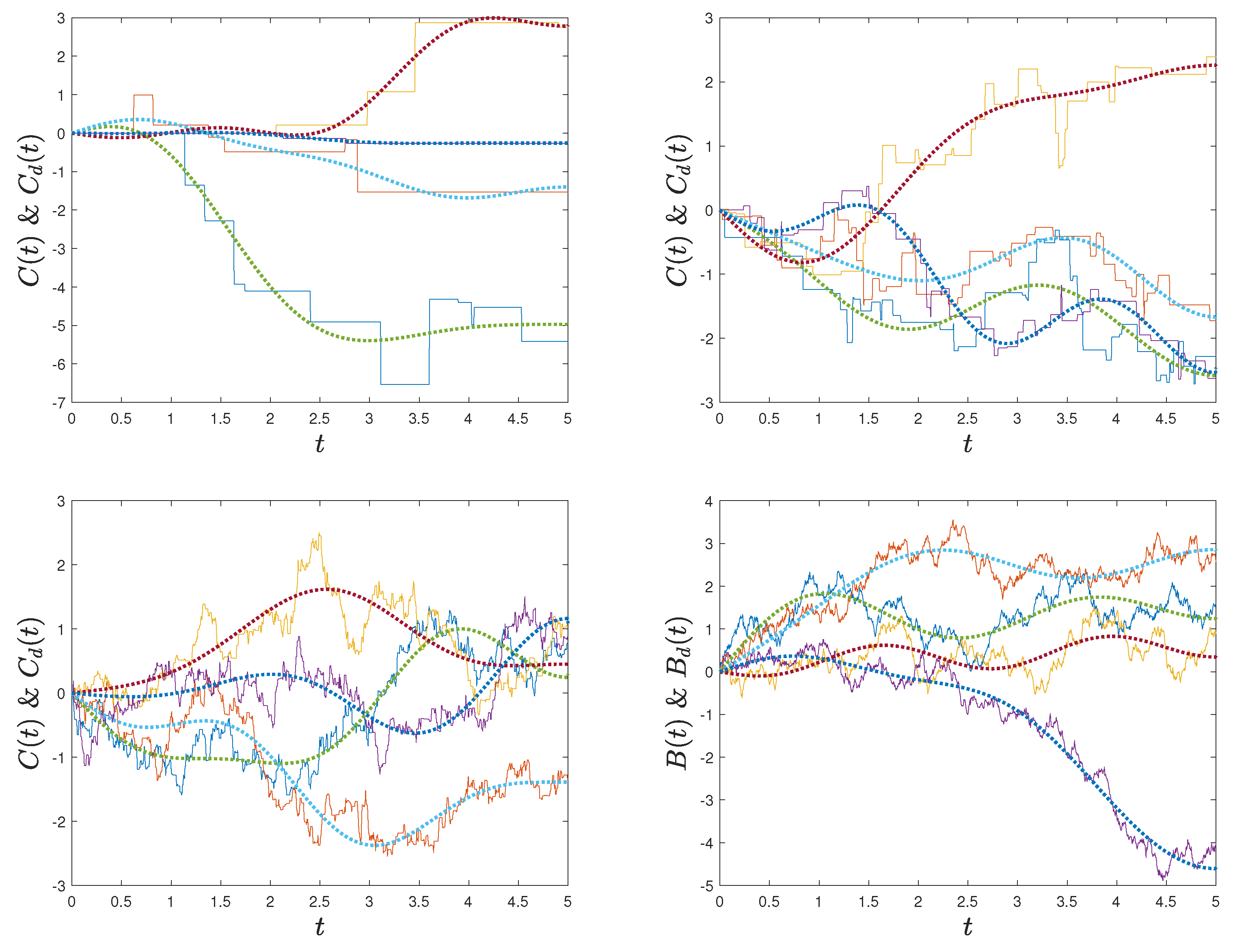
The top-left, top-right and bottom-left panels of Figure 1 show four paths of C and $C_d$ with solid and dotted lines for $\lambda =1$, 10 and 100 and stochastic dimension $d=5$. Samples of the random coefficients of $C_d$ have been calculated from (6). The paths of $C_d$ capture the trend of the corresponding paths of C even for these low stochastic dimensions. The bottom-right panel shows four paths of B and of its FD model $B_d$ with solid and dotted lines. The FD model $B_d$ of B is given by (7) with random coefficients in (6). The FD paths trace closely the target paths. The plots in the bottom-left and right panels of this figure suggest that the paths of C are similar to those of the Brownian motion for a sufficiently large intensity $\lambda$ of the Poisson process N. The above comments on the relationship between paths of $C_d$, C and B are based on visual observations. We have not proved that, e.g., the paths of C approach the paths of B as $\lambda \to \infty$.

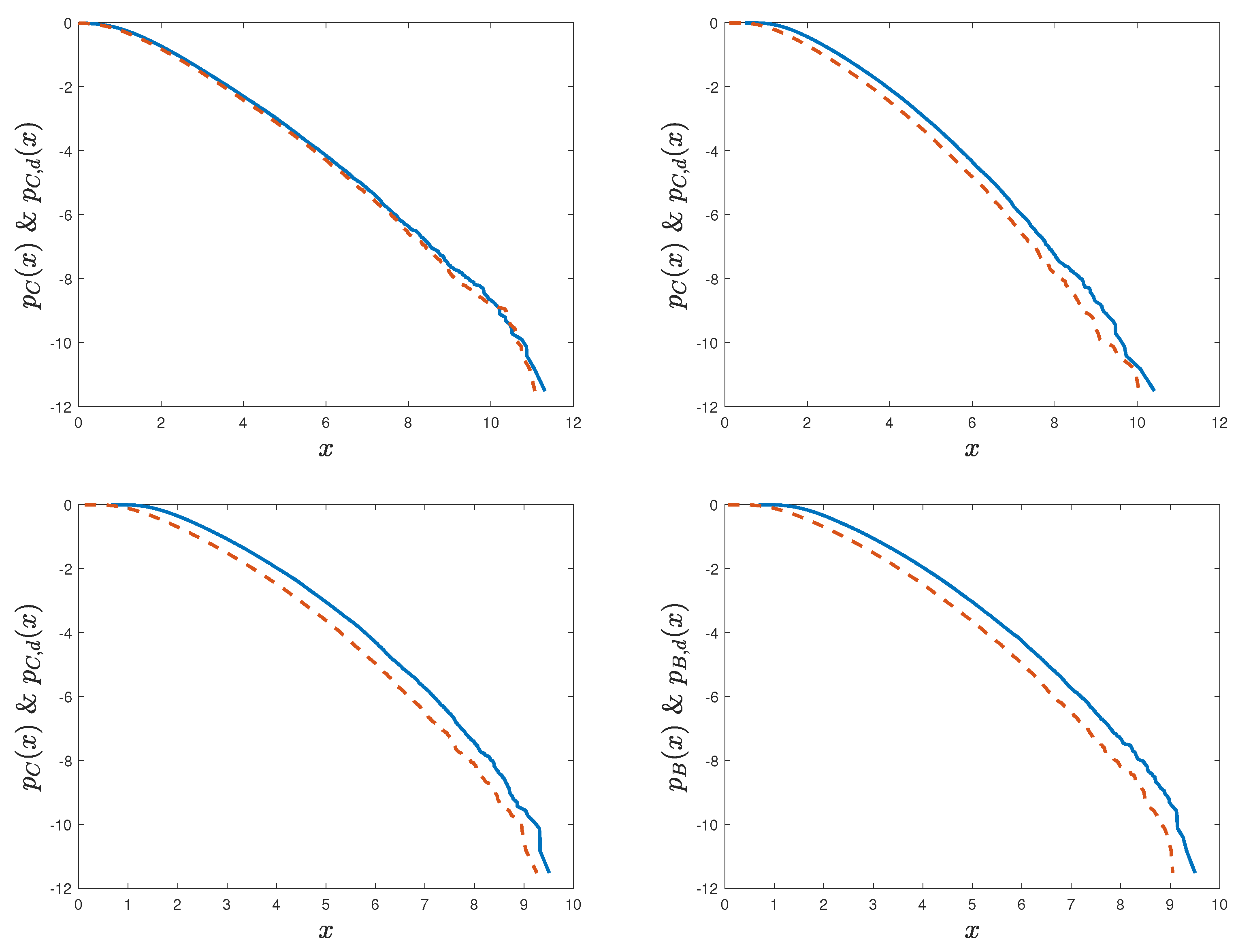
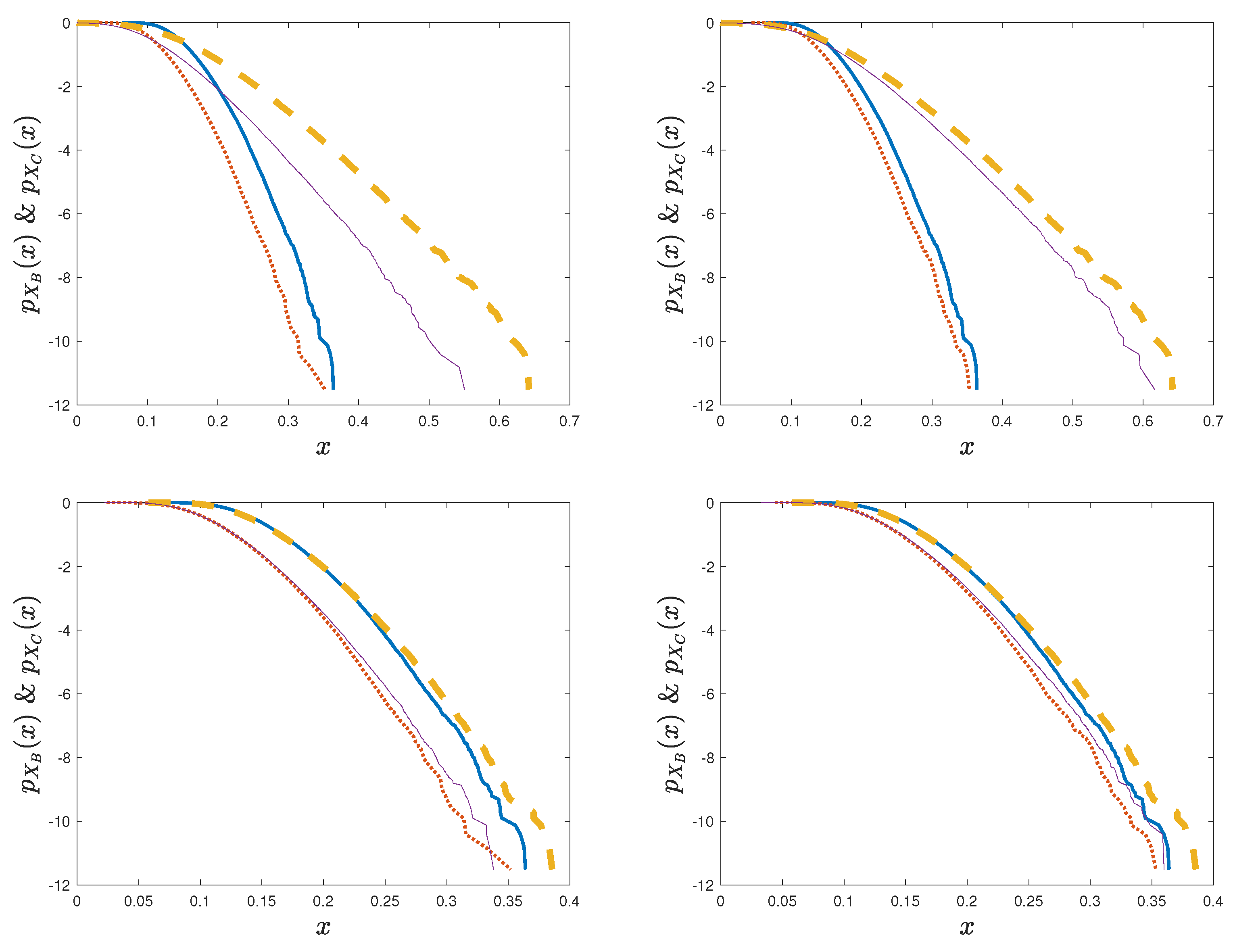
The top-left, top-right and bottom-left panels of Figure 2 display estimates of the probabilities $p_C(x)=\mathbb{P}\left({\sup }_{0\le t\le \tau }|C(t)|>x\right)$ and $p_{C,d}(x)=\mathbb{P}\left({\sup }_{0\le t\le \tau }|C_d(t)|>x\right)$ with solid and dashed lines for $\lambda =1$, 10 and 100 (top-left, top-right and bottom-left panels) and of $p_B(x)=\mathbb{P}\left({\sup }_{0\le t\le \tau }|B(t)|>x\right)$ and $p_{B,d}(x)=\mathbb{P}\left({\sup }_{0\le t\le \tau }|B_d(t)|>x\right)$ with solid and dashed lines (bottom-right panel). The stochastic dimension of the FD models $C_d$ and $B_d$ is $d=5$. The estimates are based on 100,000 independent paths of C, $C_d$, B and $B_d$. The probabilities are shown in logarithmic scale. The plots suggest that FD estimates of extremes for the stochastic dimension $d=5$ are satisfactory. That the FD estimates $p_{C,d}(x)$ of $p_C(x)$ are most accurate for $\lambda =1$ may be explained by the fact that the target process C has on average only $\lambda \tau =5$ jumps in $[0,\tau ]$ and the FD models depends on five random variables. Note also that for $\lambda =100$ the probabilities $p_{C,d}(x)$ and $p_{B,d}(x)$ and the probabilities $p_C(x)$ of $p_B(x)$ nearly coincide in agreement with Theorems 4 and 5.

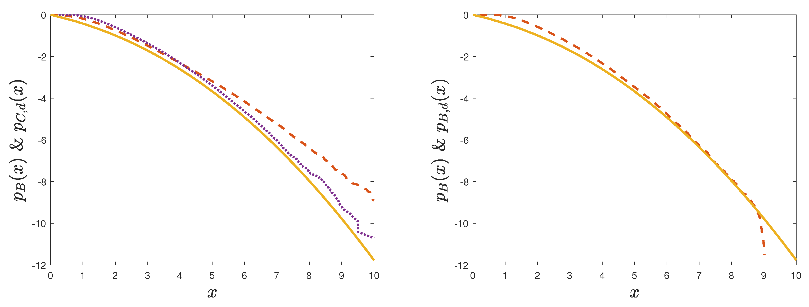
The heavy solid lines in the panels of Figure 3 display the distribution of ${\sup }_{0\le t\le \tau }\left\{B(t)\right\}$. We use this extreme random variable as quantity of interest since its distribution is know. It has the form

$$\mathbb{P}(\underset{0\le t\le \tau }{\sup }\left\{B(t)\right\}>x)=\mathbb{P}\left(T_x\le \tau \right)=2\mathrm{\Phi }\left(-2x/\sqrt{\tau }\right),x\in \mathbb{R},$$

where $\mathrm{\Phi }$ denotes the distribution of the standard Gaussian variable $N(0,1)$ and $T_x$ denotes the first time when B exceeds x in $[0,\tau ]$. The first equality holds since $\{{\sup }_{0\le t\le \tau }\left\{B(t)\right\}>x\}$ and $\{T_x\le \tau \}$ are equivalent events. For the second equality, note that

$$\mathbb{P}\left(B(\tau )>x\right)=\mathbb{P}\left(B(\tau )>x\mid T_x>\tau \right)\mathbb{P}\left(T_x>\tau \right)+\mathbb{P}\left(B(\tau )>x\mid T_x\le \tau \right)\mathbb{P}\left(T_x\le \tau \right),$$

$\mathbb{P}\left(B(\tau )>x\mid T_x>\tau \right)=0$ and $\mathbb{P}\left(B(\tau )>x\mid T_x\le \tau \right)=1/2$ by the symmetry of the Brownian motion process. We have $\mathbb{P}\left(B(\tau )>x\right)=(1/2)\mathbb{P}\left(T_x\le \tau \right)$, which gives the stated result. The dashed line in the right panel is $p_{B,d}(x)=\mathbb{P}\left({\sup }_{0\le t\le \tau }\left\{B_d(t)\right\}>x\right)$ for $d=10$. The plot suggests that $p_{B,d}(x)$ is an accurate surrogate for the target probability $p_B(x)=\mathbb{P}\left({\sup }_{0\le t\le \tau }\left\{B(t)\right\}>x\right)$. The dashed and dotted lines in the left panel are estimates of $p_{C,d}(x)=\mathbb{P}\left({\sup }_{0\le t\le \tau }\left\{C_d(t)\right\}>x\right)$ for $\lambda =1$ and 10 with stochastic dimension $d=10$. The estimates approach the probability $p_B(x)$ as $\lambda$ increases in agreement to Theorem 5. We have not increase d since this stochastic dimension seems to be sufficiently large. The probabilities in this figure are shown in the logarithmic scale.

Figure 3. Probability $p_B(x)=\mathbb{P}\left({\sup }_{0\le t\le \tau }\left\{B(t)\right\}>x\right)$ (heavy solid lines) and estimates of $p_{C,d}(x)=\mathbb{P}\left({\sup }_{0\le t\le \tau }\left\{C_d(t)\right\}>x\right)$ (left panel, dashed and dotted lines for $\lambda =1$ and 10) and of $p_{B,d}(x)=\mathbb{P}\left({\sup }_{0\le t\le \tau }\left\{B_d(t)\right\}>x\right)$ (right panel, dashed line) for $d=10$. All probabilities are in logarithmic scale.

Figure 3. Probability $p_B(x)=\mathbb{P}\left({\sup }_{0\le t\le \tau }\left\{B(t)\right\}>x\right)$ (heavy solid lines) and estimates of $p_{C,d}(x)=\mathbb{P}\left({\sup }_{0\le t\le \tau }\left\{C_d(t)\right\}>x\right)$ (left panel, dashed and dotted lines for $\lambda =1$ and 10) and of $p_{B,d}(x)=\mathbb{P}\left({\sup }_{0\le t\le \tau }\left\{B_d(t)\right\}>x\right)$ (right panel, dashed line) for $d=10$. All probabilities are in logarithmic scale.

7.2. Additive White Noise

Let $X_C$ and $X_B$ be real-valued processes defined by the stochastic differential equations

$$\begin{array}{c}d{X}_C(t)=\alpha X_C(t)dt+\sqrt{2\alpha }dC(t)\mathrm{and}\hfill \\ \hfill \\ d{X}_B(t)=\alpha X_B(t)dt+\sqrt{2\alpha }dB(t)\hfill \end{array}$$

(9)

where $\alpha >0$ and the jumps of C are such that C and B have the same first two moments. If the two equations have the same initial condition assumed to be independent of C and B, then $X_C$ and $X_B$ also have the same first two moments. Denote by $X_{C,d}$ and $X_{B,d}$ the solutions of the above equations with $C_d$ and $B_d$ in place of C and B.

According to our theoretical arguments (Theorems 1–4), the FD models $B_d$ and $C_d$ converge weakly to the Brownian motion and the compound Poisson processes B and C as $d\to \infty$. Since the I/O maps defined by the above equations are continuous, the weak convergences $C_d⟹C$ and $B_d⟹B$ imply $X_{C,d}⟹X_C$ and $X_{B,d}⟹X_B$ as $d\to \infty$ by Theorem 6. This means that the distributions of ${\sup }_{0\le t\le \tau }|X_C(t)|$ and ${\sup }_{0\le t\le \tau }|X_B(t)|$ can be approximated by those of ${\sup }_{0\le t\le \tau }|X_{C,d}(t)|$ and ${\sup }_{0\le t\le \tau }|X_{B,d}(t)|$ for a sufficiently large d. Moreover, the distribution of ${\sup }_{0\le t\le \tau }|X_B(t)|$ can be approximated by that of ${\sup }_{0\le t\le \tau }|X_{C,d}(t)|$ for a sufficiently large stochastic dimension d and intensity parameter $\lambda$.

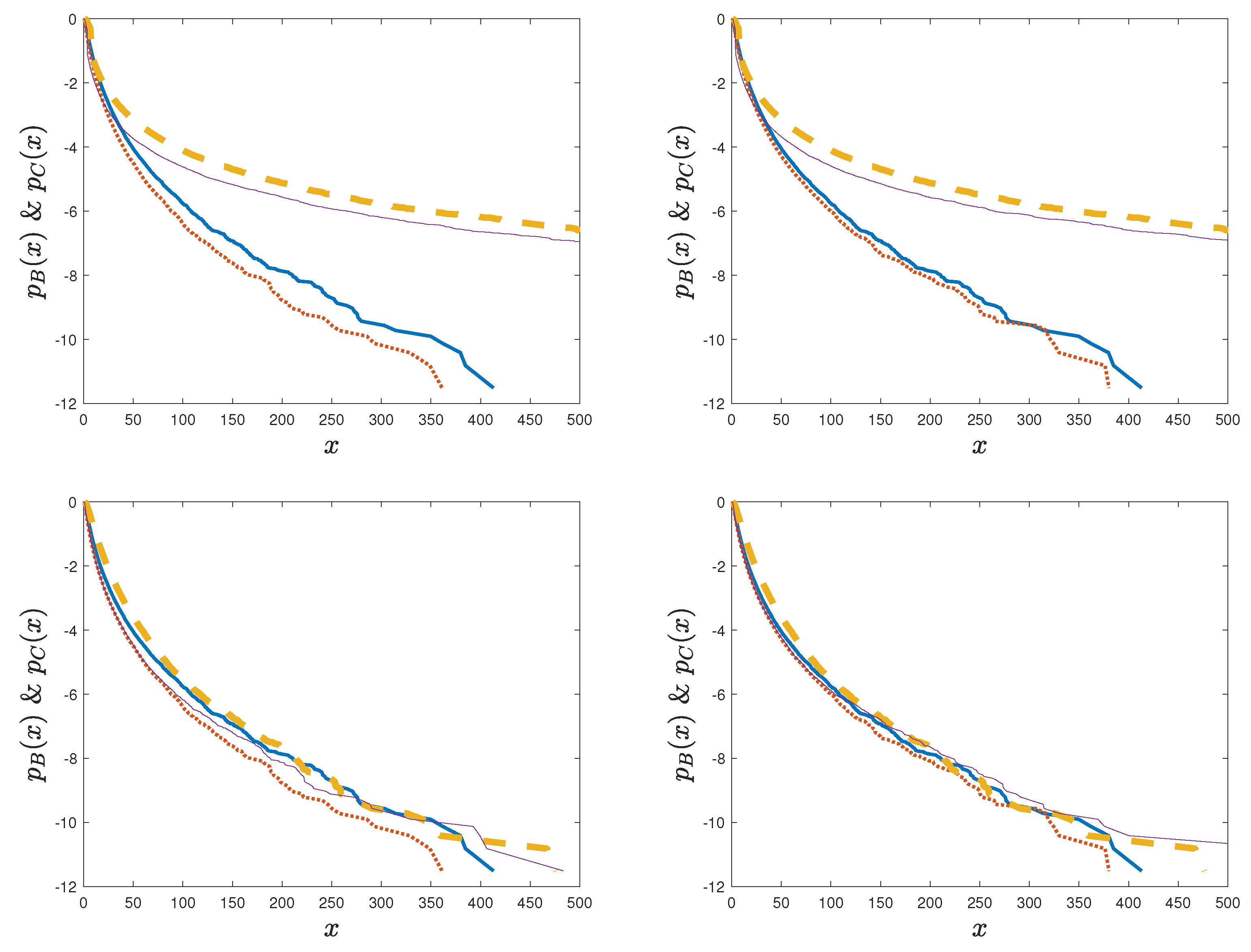
The following numerical results are for $\alpha =1$, $\lambda =1;40$ and $d=10;30$. The estimates are based on 100,000 independent paths of B, C, $B_d$ and $C_d$. The heavy solid and dashed lines in Figure 4 are estimates of the probabilities $p_{X_B}(x)=\mathbb{P}\left({\sup }_{0\le t\le \tau }|X_B(t)|>x\right)$ and $p_{X_C}(x)=\mathbb{P}\left({\sup }_{0\le t\le \tau }|X_C(t)|>x\right)$ while the dotted and the thin continuous lines are estimates of $p_{X_{B,d}}(x)=\mathbb{P}\left({\sup }_{0\le t\le \tau }|X_{B,d}(t)|>x\right)$ and $p_{X_{C,d}}(x)=\mathbb{P}\left({\sup }_{0\le t\le \tau }|X_{C,d}(t)|>x\right)$. The intensity of the Poisson process in the top panels is $\lambda =1$. As expected, responses to Poisson and Gaussian white noise inputs differ. These plots also show that the estimates of the probabilities $p_{X_{B,d}}(x)$ and $p_{X_{C,d}}(x)$ improve with d. The bottom panels show that, for $\lambda =40$, the probabilities $p_{X_C}(x)$ and $p_{X_B}(x)$ can be substituted for each other in agreement to Theorems 4–6. Also, for a sufficiently large $\lambda$ and d, $p_{X_{C,d}}(x)$ can be used as a surrogate for $p_{X_B}(x)$ and $p_{X_C}(x)$. The probabilities in this figure are displayed in the logarithmic scale.

7.3. Multiplicative Noise

Let $X_B$ denote the geometric Brownian motion process defined by the Itô stochastic differential equation

$$d{X}_B(t)=c{X}_B(t)dt+\sigma X_B(t)dB(t),t\ge 0,$$

(10)

with solution

$$X_B(t)=x_0\exp \left[(c-{\sigma }^2/2)t+\sigma B(t)\right],t\ge 0$$

(11)

for the initial state $X_B(0)=x_0$, where c and $\sigma$ are real constants. Its FD version $X_{B,d}$ is the solution of the Stratonovich SDE

$$\begin{array}{c}d{X}_{B,d}(t)=(c-{\sigma }^2/2)X_{B,d}(t)dt+\sigma X_{B,d}(t)\circ d{B}_d(t),t\ge 0,\mathrm{or}\hfill \\ \hfill \\ {\dot{X}}_{B,d}(t)=(c-{\sigma }^2/2)X_{B,d}(t)+\sigma X_{B,d}(t)\circ {\dot{B}}_d(t),t\ge 0\hfill \end{array}$$

(12)

where $B_d(t)={\sum }_{k=1}^d{Z}_{B,k}{\phi }_k(t)$ is an FD model of the Brownian motion B, the symbol ∘ indicates that the equation has to be interpreted in the Stratonovich sense and dots above $X_B$ and $B_d$ denote differentiation with respect to time. The drift of this equation is that of (10) modified by the Wong–Zakai correction term [13] (Sect. 4.7.1.2). Its solution results by following the rules of the classical calculus and has the expression

$$X_{B,d}(t)=x_0\exp \left[(c-{\sigma }^2/2)t+\sigma B_d(t)\right],t\ge 0.$$

(13)

Since $B_d$ converges almost surely (a.s.) to B in the metric of the space of real-valued continuous functions [12] (Theorem 5.17) and the I/O map is continuous, $X_{B,d}\to X_B$ a.s. in the metric of this space as $d\to \infty$. This means that paths and extremes of $X_{B,d}$ can be used as surrogates for those of $X_B$ provided that the stochastic dimension d is sufficiently large.

Let $X_C$ be $X_B$ in (11) with C in place of B, i.e.,

$$X_C(t)=x_0\exp \left[(c-{\sigma }^2/2)t+\sigma C(t)\right],t\ge 0,$$

(14)

where C denotes the compound Poisson process in (1) with jumps $Y_k\sim N(0,1/\lambda )$. Since the continuous maps $B\mapsto X_B$ in (11) and $C\mapsto X_C$ in (14) have the same form and $C⟹B$ as $\lambda \to \infty$, we have $X_C⟹X_B$ as $\lambda \to \infty$ by the continuous mapping theorem. By analogy with the SDE of $X_B$, it is tempting to assume that $X_C$ satisfies the SDE $d{X}_C(t)=c{X}_C(t-)dt+\sigma X_C(t-)dC(t)$, where $X(t-)={\lim }_{s\uparrow t}X(s)$ denotes the left limit of X at time t. It turns out that $X_C$ is the solution of a different SDE.

The SDE satisfied by $X_C$ results from the multivariate Itô formula, see [16] (Sect. 5.3) and [17] (Theorem 33, p. 74), applied to its definition in (14). Since $X_C$ is a function of time t and the compound Poisson process $C(t)$, the expression of the difference $X_C(t)-X_C(0)$ has three types of terms. The first type of terms involve integrals whose integrands are partial derivatives of $X_C$ with respect to t and $C(t)$; the second type of terms consists of integrals whose integrators are the continuous parts of the quadratic variations $[I,I]$, $[I,C]$ and $[C,C]$, which are zero, where I denotes the identity function; and the third is a summation related to the jumps of $X_C$ and C, i.e.,

$$\begin{array}{cc}\hfill X_C(t)-X_C(0)& ={\int }_0^t(c-{\sigma }^2/2)X_C(s-)ds+{\int }_0^t\sigma f{X}_C(s-)dC(s)\hfill \\ \hfill & +\sum _{0<s\le t}\left[X_C(s)-X_C(s-)-\sigma X_C(s-)\Delta C(s)\right]\hfill \end{array}$$

where $\Delta C(s)=C(s)-C(s-)$ is the jump of C at time s and $C(s-)={\lim }_{u\uparrow s}C(u)$ is the left limit of C at time s. Since $\Delta C(s)\ne 0$ only at the jump times $\left\{T_k\right\}$ of C, we have

$${\int }_0^t\sigma X_C(s-)dC(s)=\sum _{k=1}^{N(t)}\sigma X_C(T_k-)Y_k=\sum _{0<s\le t}\sigma X_C(s-)\Delta C(s)$$

so that the above integral equation becomes

$$X_C(t)-X_C(0)={\int }_0^t(c-{\sigma }^2/2)X_C(s-)ds+\sum _{0<s\le t}\left[X_C(s)-X_C(s-)\right].$$

The definition of $X_C$ in (14) gives

$$X_C(T_k)=x_0\exp [(c-{\sigma }^2/2)T_k+\sigma (\sum _{r=1}^{N(T_k)-1}{Y}_r+Y_k)]=X_c(T_k-)e^{\sigma Y_k}$$

since $\exp \left[(c-{\sigma }^2/2)T_k\right]=\exp \left[(c-{\sigma }^2/2)T_k-\right]$ so that

$$\begin{array}{cc}\hfill \sum _{0<s\le t}\left[X_C(s)-X_C(s-)\right]& =\sum _{k=1}^{N(t)}{X}_C(T_k-)\left(e^{\sigma Y_k}-1\right)=\sum _{k=1}^{N(t)}{X}_C(T_k-)\Delta \tilde{C}(s)\hfill \\ \hfill & ={\int }_0^t{X}_C(s-)d\tilde{C}(s),\hfill \end{array}$$

where $\tilde{C}(s)={\sum }_{k=1}^{N(s)}{\tilde{Y}}_k$ is a compound Poisson process with jumps ${\tilde{Y}}_k=e^{\sigma Y_k}-1$ at the jump times $T_k$ of C. Then, $X_C$ satisfies the stochastic integral equation

$$X_C(t)-X_C(0)={\int }_0^t(c-{\sigma }^2/2)X_C(s-)ds+{\int }_0^t{X}_C(s-)d\tilde{C}(s)$$

or, equivalently, the stochastic integral equation

$$X_C(t)-X_C(0)={\int }_0^{t}c{X}_C(s-)ds+{\int }_0^t{X}_C(s-)d{C}^{*}(s)$$

where $C^{*}(t)=\tilde{C}(t)-E\left[\tilde{C}(t)\right]=\tilde{C}(t)-{\sigma }^{2}t/2$ constitutes the (asymptotic) compensated version of $\tilde{C}$ since

$$\begin{array}{cc}\hfill E\left[C^{*}(t)\right]& =E\left[\tilde{C}(t)\right]-{\sigma }^{2}t/2=E\left\{E\left[\tilde{C}(t)\mid N(t)\right]\right\}-{\sigma }^{2}t/2=E\left\{N(t)E\left[{\tilde{Y}}_1\right]\right\}]-{\sigma }^{2}t/2\hfill \\ \hfill & =\lambda t\left(e^{{\sigma }^2/(2\lambda )}-1\right)-{\sigma }^{2}t/2\to 0,rmas\lambda \to \infty .\hfill \end{array}$$

The differential versions of the above integral equations have the forms

$$\begin{array}{cc}\hfill d{X}_C(t)& =(c-{\sigma }^2/2)X_C(t-)dt+X_C(t-)d\tilde{C}(t)\mathrm{or},\mathrm{equivalently},\hfill \\ \hfill d{X}_C(t)& =c{X}_C(t-)dt+X_C(t-)d{C}^{*}(t)\hfill \end{array}$$

which differ from $d{X}_C(t)=c{X}_C(t-)dt+X_C(t-)dC(t)$ suggested by intuition. The estimates of the probability $p_{X_C}(x)$ in Figure 5 have been obtained from solutions of the differential equations of $X_C$. They have been validated by using the definition of $X_C$ in (14) and paths of the compound Poisson process C.

Consider now the process $X_{C,d}$ defined by

$$X_{C,d}(t)=x_0\exp \left[(c-{\sigma }^2/2)t+\sigma C_d(t)\right],t\ge 0,$$

(15)

where $C_d={\sum }_{k=1}^d{Z}_{C,k}{\phi }_k(t)$ is an FD model of C. The differentiation of (15), which is performed by following the rules of the classical calculus, gives ${\dot{X}}_{C,d}(t)=(c-{\sigma }^2/2)X_{C,d}(t)+\sigma X_{C,d}(t){\dot{C}}_d(t)$, which has the form of the differential equation of $X_{B,d}$ in (12). Note that the convergence $C_d⟹C$ implies $X_{C,d}⟹X_C$ as $d\to \infty$ by the continuous mapping theorem and that $X_{C,d}⟹X_B$ as $d,\lambda \to \infty$ by Theorem 6.

The plots of Figure 5 are for $c=1$, $\sigma =0.8$, $\tau =2$, integration time step $\Delta t=2/1000$ and 100,000 independent paths of $X_B$, $X_{B,d}$, $X_C$ and $X_{C,d}$. The top and bottom panels are for $\lambda =0.5$ and 20. The left and right panels are for $d=5$ and 20. The heavy solid and dashed lines are the probabilities $p_{X_B}(x)=\mathbb{P}\left({\sup }_{0\le t\le \tau }|X_B(t)|>x\right)$ and $p_{X_C}(x)=\mathbb{P}\left({\sup }_{0\le t\le \tau }|X_C(t)|>x\right)$. Their FD approximations $p_{X_{B,d}}(x)=\mathbb{P}\left({\sup }_{0\le t\le \tau }|X_{B,d}(t)|>x\right)$ and $p_{X_{C,d}}(x)=\mathbb{P}\left({\sup }_{0\le t\le \tau }|X_{C,d}(t)|>x\right)$ are displayed in heavy dotted and thin solid lines. The logarithmic scale is used for all probabilities.

The plots are consistent with Theorems 4–6. The top panels show that extremes of $X_C;X_{C,d}$ differ from those of $X_B;X_{B,d}$, an expected result since $\lambda =0.5$ is small so that Theorem 4 predicting that C is a surrogate of B does not apply. The increase of the stochastic dimension from $d=5$ to $d=20$ shows that the extremes of $X_{B,d}$ and $X_{C,d}$ better approximate the corresponding extremes of $X_B$ and $X_C$ in agreement with Theorems 2 and 6. The improvement of the FD estimates is more pronounced for the estimates of $p_{X_{B,d}}(x)$. The bottom panels suggest that $\lambda =20$ is sufficiently large in this example such that the distributions of extremes of $X_C$ and $X_B$ are similar and that these extremes can be approximated by those of the FD models $X_{C,d}$ and $X_{B,d}$ in agreement with Theorems 5 and 6. The increase of the stochastic dimension from $d=5$ to $d=20$ improves slightly the performance of the estimates of the extremes of the FD models.

7.4. Relationship to Current Integration Algorithms

We examine three aspects of the proposed and the current methods for integrating SDEs with GWN and PWN inputs. It is not possible to rate the performance of these methods precisely since it depends on the type of the posed SDE and the quantities of interest, e.g., solution moments, marginal distributions, or extremes. We only present features and limitations of these methods.

• Computational speed: It is difficult to make a general statement on the computational efficiency of the proposed and current integration algorithms. The Euler integration scheme of the current methods can be implemented directly for SDEs with GWN. However, an Euler-like integration scheme requires extensive preparation for solving SDEs with PWN. Moreover, the integration time step of these schemes needs to be sufficiently small such the probability of having two or more Poisson jumps in a single time step be nearly zero. This means that the computational time for SDEs subjected to PWN inputs with frequent jumps can be significant since the required integration time step has to be very small.

The implementation of the proposed methods requires first to construct FD models for the Brownian motion and the compound Poisson processes in (7). The basis functions of these FD models are available analytically and samples of their random coefficients result by, e.g., projecting paths of the Brownian motion and the compound Poisson processes on the basis functions. The generation of paths of these processes and their projection on basis functions involve elementary calculations. Paths of FD solutions are delivered by standard ODE algorithms. Note that the estimates of the distribution of extremes of FD models of compound Poisson process in Figure 2 are accurate for a broad range of Poisson intensities and the same stochastic dimension.

• Model dimension: We have proved the convergence of the distributions of functionals of FD solutions to those of target solutions as $d\to \infty$. The rate of convergence would be required to determine the model dimension d such that the error does not exceed a specified value. Since we do not have the convergence rate, we estimate the distribution of, e.g., the extreme random variable ${\sup }_{0\le t\le \tau }|X_d(t)|$, for several increasing values of the stochastic dimension d and approximate the distribution of ${\sup }_{0\le t\le \tau }|X(t)|$ by the smallest d beyond which the FD-based distribution changes insignificantly, see Figure 4. The starting valued of d for this iteration can be that for which the FD input models contain most energy of the processes they represent. We also note that the stochastic dimension of the current integration methods is given by the number n of the time steps and that n is much larger than the stochastic dimension d of the proposed method. Moreover, we have obtained accurate solutions for low stochastic dimensions, as seen in Figure 1, Figure 2, Figure 3, Figure 4 and Figure 5.
• Scalability: If the solution X of the posed SDE is a vector-valued process and the input consists of several Brownian motions and/or compound Poisson processes, the implementation of the proposed integration algorithm is conceptually similar. The simplest method is to construct FD models as in (7) for the individual components of the input, which may or may not have the same stochastic dimensions. The relationships between the components of the FD models are captured by the dependence between the random coefficients of the FD components. Once the input FD models have been constructed, ODE solvers can be used as previously to generate paths of the FD solutions.

We conclude this subsection by mentioning that the proposed method gives conditions under which the distributions of extreme solutions of SDEs can be approximated by those of corresponding FD solutions. This is essential for applications since the distribution of quantities of interest such as the random variable ${\sup }_{0\le t\le \tau }|X(t)|$, which is rarely available analytically and cannot be obtained numerically, can be approximated by the distribution of the corresponding FD extreme ${\sup }_{0\le t\le \tau }|X_d(t)|$, which can be estimated from FD solution paths generated by standard numerical algorithms. In contrast, the construction of such estimates from the solutions of current methods require to postulate the behavior of the solution between the times of the recurrence formulas, which is unknown.

8. Conclusions

A method has been developed for integrating stochastic differential equations (SDEs) with Gaussian (GWN) and Poisson (PWN), which is conceptually different from the current integration methods. As for the current methods, the GWN and the PWN inputs are interpreted as the formal derivatives of the Brownian motion and compound Poisson processes. The current methods solve discrete time versions of the posed SDEs by using different recurrence formulas for Gaussian and Poisson white noises. In contrast, the proposed method solves the posed SDEs for finite dimensional (FD) models of the compound Poisson and Brownian motion processes, i.e., finite sums of d deterministic functions of time, referred to as basis functions, weighted by random coefficients, by using a single algorithm for both types of noises. The number d of random coefficients of the FD input models gives their stochastic dimension.

The implementation of the proposed method requires to first construct FD models for the Brownian motion and the compound Poisson processes. The construction involves elementary calculations since the basis functions of the models are available analytically, samples of their random coefficients can be obtained by projecting Brownian and Compound Poisson paths on the basis functions and efficient algorithms are available for generating large sets of paths of these processes.

Standard ODE solvers have been employed to calculate paths of the solutions of the posed SDEs from paths of the FD input models, referred to as FD solutions. It was shown that statistics of continuous functionals of the FD solutions can be used as surrogates for those of the target solutions under some conditions provided that the stochastic dimension is sufficiently large. This is a notable feature of the method since the distributions of functionals of solutions of SDEs with GWN and PWN are rarely available analytically and cannot be obtained numerically, while the distributions of corresponding functionals of FD solutions can be estimated from their paths, which can be generated by standard numerical methods. The implementation and the performance of the proposed method based on FD input models have been illustrated by examples involving compound Poisson and Brownian motion processes, SDEs with additive GWN and PWN, and SDEs with multiplicative GWN and PWN. The performance of the proposed method is remarkable and consistent with the theoretical results in the paper.