Scalable Likelihood Inference for Student-t Copula Count Time Series

Abstract

Count time series often exhibit extremal dependence that may not be adequately captured by Gaussian copula models. We develop a likelihood-based framework for count-valued time series using Student-t copulas with latent ARMA dependence. The latent process is constructed through a scale-mixture representation of a Gaussian ARMA process, preserving the second-order dependence structure while introducing tail dependence and greater persistence of extreme events. Likelihood inference requires evaluating high-dimensional truncated multivariate t probabilities, which is computationally demanding under heavy tails and strong serial dependence. To address this challenge, we develop scalable likelihood approximations tailored to the time series structure. In particular, we formulate a time series version of minimax exponential tilting for multivariate t probabilities, termed Time Series Minimax Exponential Tilting (TMET), which exploits the exact conditional representation of the latent ARMA process. The resulting algorithm reduces computational complexity from cubic to near-linear in the series length while retaining the high accuracy of minimax exponential tilting. For comparison, we also extend two widely used Gaussian copula approximations—the continuous extension (CE) method and the Geweke–Hajivassiliou–Keane (GHK) simulator—to the Student-t copula setting. Simulation studies show that TMET outperforms CE and GHK, particularly under strong dependence, heavy tails, and low-count regimes. The framework also supports predictive inference and residual diagnostics. An application to weekly rotavirus counts illustrates how the Student-t copula provides a flexible extension of the Gaussian copula while retaining stable inference even when tail dependence is weak or absent.

1. Introduction

Copula models provide a flexible framework for constructing multivariate and time-series models by separately modeling the marginal and dependence structures [1]. For count-valued time series, copula models are particularly attractive: a continuous latent process, typically Gaussian, is mapped to observed counts through marginal quantile transformations, enabling likelihood-based inference while retaining a familiar linear-process structure [2,3,4]. In time series applications, the latent process is typically endowed with parametric serial dependence, such as an ARMA structure, allowing temporal dependence to be modeled separately from the marginal distributions. Recent work on count time series has also developed alternative non-copula autoregressive constructions, including threshold and high-dimensional banded integer-valued models [5,6].

The Gaussian copula remains the dominant choice because its conditional moments are analytically tractable and simulation is computationally inexpensive. However, Gaussian dependence cannot reproduce joint extremes: its tail dependence coefficients vanish except under perfect correlation [7]. Many applications involving count data, such as insurance claims, disease incidence, cyber events, and heat-wave occurrences, exhibit large observations that occur in persistent clusters. Such behavior reflects temporal tail dependence, which Gaussian copulas cannot capture because of their zero tail dependence property [8].

The Student-t copula offers a natural extension by introducing a degrees-of-freedom parameter $\nu$ that induces nonzero tail dependence, while recovering the Gaussian copula as $\nu \to \infty$. Despite its wide use in cross-sectional risk modeling [9,10], its application to count-valued time series has been absent. The main barrier is computational, since likelihood-based inference requires evaluation of high-dimensional truncated multivariate t probabilities, which are more challenging than their Gaussian counterparts. In addition, conditional variances in t processes depend on the realized latent history, breaking the constant variance structure that enables efficient Gaussian filtering, and simulation from truncated t distributions is considerably more expensive than from truncated Gaussian distributions.

Existing numerical methods for multivariate t probabilities, including separation-of-variables algorithms [11] and minimax exponential tilting (MET) [12], have not been adapted to latent t copula time series. The recent Vecchia-based MET method of [13] achieves near-linear complexity for spatial Gaussian models, but may be biased for time series with certain latent structures, such as moving averages [14]. Consequently, existing software for copula time series and spatial data (e.g., gcmr [15] and gcKrig [16]) remains restricted to Gaussian copulas despite the potential advantages of modeling temporal tail dependence.

Motivated by the computational and inferential challenges posed by heavy-tailed latent dependence in count-valued time series, we develop the first comprehensive framework for likelihood inference, prediction, and model diagnostics in Student-t copula count time series. A central contribution of this paper is the formulation of a time series minimax exponential tilting (TMET) algorithm for Student-t copula models. While MET was originally developed for multivariate Student-t and Gaussian rectangle probabilities, its integration within copula models for count time series with a Student-t latent process has not previously been studied. By exploiting the scale-mixture representation of the multivariate t distribution together with the exact conditional structure of causal and invertible ARMA processes, we show that this construction preserves the near-linear computational footprint of Gaussian TMET in [14], while targeting the more computationally demanding heavy-tailed likelihood. To ensure numerical stability in the tilting optimization, we introduce a Levenberg–Marquardt solver with preconditioned conjugate gradient inner iterations for estimating the tilting parameters. This replaces the gradient-based scheme used in earlier Gaussian TMET implementations and yields reliable convergence across a wide range of dependence structures, tail indices, and marginal discretization levels.

An additional contribution of this paper is a formal construction of a t–ARMA process suitable for copula-based count time series models. While t copulas with ARMA dependence are often specified solely through their correlation structure, an explicit time-domain construction of the associated latent process is rarely discussed. We show that a t–ARMA process can be generated through a scale-mixture representation of a causal and invertible Gaussian ARMA process, thereby preserving the full linear time series structure, including the difference equation, causality, and invertibility, while inducing heavy-tailed behavior. This construction yields tractable conditional moments and supports efficient likelihood approximation, inference, and prediction.

A further contribution is the extension of two previously studied Gaussian copula approximations—the continuous extension (CE) method and the Geweke–Hajivassiliou–Keane (GHK) simulator—to the Student-t copula setting. To our knowledge, these approximations have not previously been developed, implemented, or systematically evaluated for t copula count time series. This allows a unified comparison of CE-, GHK-, and MET-based approaches under heavy-tailed latent dependence. Through extensive simulation studies, we provide systematic evaluations of likelihood accuracy, computational efficiency, and inferential performance for Student-t copula count time series. The results show that TMET consistently achieves MET-level accuracy while remaining computationally scalable in regimes where CE and GHK exhibit substantial bias or instability. Taken together, these developments yield the first fully operational and scalable likelihood framework for t copula count time series, broadening the applicability of copula-based models to discrete data characterized by clustered extremes, strong serial dependence, and heavy tails, features that are not accommodated by Gaussian copulas or existing approximate likelihood methods.

The remainder of the paper is organized as follows. Section 2 reviews multivariate Student-t distributions and t processes, focusing on the construction of t–ARMA processes, and the Student-t copula. Section 3 introduces the t copula model for count time series and presents two versions of its likelihood. Section 4 reviews existing computational approaches for likelihood approximation, including the continuous extension (CE), the Geweke–Hajivassiliou–Keane (GHK) simulator, and the efficient computation of the conditional quantities required by these approximations. Section 5 develops the time series minimax exponential tilting (TMET) method, a scalable implementation of exponential tilting for latent t–ARMA processes. Section 6 reports the results of a simulation study comparing likelihood accuracy, computational cost, and maximum likelihood estimation under different likelihood approximations. Section 7 discusses inference and predictive methods, and Section 8 presents model diagnostic tools. Section 9 illustrates the methodology through an application to weekly rotavirus count data. Section 10 concludes with a discussion and directions for future research.

2. Multivariate t Distributions, Processes, and Copulas

We briefly review the definitions and properties of t distributions, t processes, and t copulas needed for the construction of our count time series model. A detailed background can be found in [8,17,18,19].

2.1. Multivariate t Distributions

The multivariate t distribution is a heavy-tailed analogue of the multivariate normal distribution. Let $n\in \mathbb{N}$, $\nu >0$, and $\mathit{\mu }\in {\mathbb{R}}^n$, and let $\mathbf{\Sigma }$ be a positive-definite $n\times n$ matrix. A random vector $\mathit{V}=(V_1,\dots ,V_n)$ has an n-variate t distribution with $\nu$ degrees of freedom, location $\mathit{\mu }$, and scale $\mathbf{\Sigma }$ if its pdf is given by

$${\tau }_n(\mathit{v};\nu ,\mathit{\mu },\mathbf{\Sigma })={\displaystyle \frac{\mathrm{\Gamma }\left(\frac{\nu +n}{2}\right)}{\mathrm{\Gamma }\left(\frac{\nu }{2}\right){\left(\nu \pi \right)}^{n/2}{\left|\mathbf{\Sigma }\right|}^{1/2}}}{\left[1+{\displaystyle \frac{1}{\nu }}{(\mathit{v}-\mathit{\mu })}^{\top }{\mathbf{\Sigma }}^{-1}(\mathit{v}-\mathit{\mu })\right]}^{-(\nu +n)/2},$$

(1)

where $\mathrm{\Gamma }(·)$ is the gamma function and $\left|\mathbf{\Sigma }\right|$ is the determinant of $\mathbf{\Sigma }$. We write $\mathit{V}\sim t_n(\nu ,\mathit{\mu },\mathbf{\Sigma })$ to denote this distribution. When $n=1$, $\mathit{\mu }=0$, and $\mathbf{\Sigma }=1$, (1) reduces to the pdf of the standard t distribution; in this case, the density and distribution are denoted by $\tau (v;\nu )$ and $t\left(\nu \right)$, respectively. The heaviness of the tails is controlled by $\nu$, and the $t_n(\nu ,\mathit{\mu },\mathbf{\Sigma })$ distribution converges to the ${\mathrm{N}}_n(\mathit{\mu },\mathbf{\Sigma })$ distribution as $\nu \to \infty$ [17]. Because smaller values of $\nu$ produce heavier tails, t distributions can provide robust models for data exhibiting extreme deviations from their averages.

Scale-mixture Representation. A key property of t distributions is their representation as scale mixtures of normals [17]. For any random vector $\mathit{V}\sim t_n(\nu ,\mathit{\mu },\mathbf{\Sigma })$

$$\mathit{V}\stackrel{d}{=}\mathit{\mu }+{\displaystyle \frac{\mathit{Z}}{W/\sqrt{\nu }}},$$

(2)

where

$$\mathit{Z}\sim {\mathrm{N}}_n(\mathbf{0},\mathbf{\Sigma }),W\sim {\chi }_{\nu },\mathit{Z}\mathrm{and}W\mathrm{independent}.$$

The notation ${\mathit{X}}_1\stackrel{d}{=}{\mathit{X}}_2$ means that the random vectors ${\mathit{X}}_1$ and ${\mathit{X}}_2$ have the same distribution, and ${\chi }_{\nu }$ denotes the distribution of the square root of a chi-squared random variable with $\nu$ degrees of freedom. Equivalently

$$\mathit{V}\mid W=w\sim {\mathrm{N}}_n\left(\mathit{\mu },{\displaystyle \frac{\nu }{w^2}}\mathbf{\Sigma }\right),W\sim {\chi }_{\nu }.$$

This representation will be used in later sections for likelihood approximation and simulation. It follows from this representation that, for $\nu >2$

$$E\left(\mathit{V}\right)=\mathit{\mu },\mathrm{var}\left(\mathit{V}\right)={\displaystyle \frac{\nu }{\nu -2}}\mathbf{\Sigma }.$$

Conditional Distributions. Let $\mathit{V}\sim t_n(\nu ,\mathit{\mu },\mathbf{\Sigma })$ and suppose that $\mathit{V}$, $\mathit{\mu }$, and $\mathbf{\Sigma }$ are partitioned as

$$\mathit{V}=\left(\begin{array}{c}{\mathit{V}}_1\\ {\mathit{V}}_2\end{array}\right),\mathit{\mu }=\left(\begin{array}{c}{\mathit{\mu }}_1\\ {\mathit{\mu }}_2\end{array}\right),\mathrm{and}\mathbf{\Sigma }=\left(\begin{array}{cc}{\mathbf{\Sigma }}_{11}& {\mathbf{\Sigma }}_{12}\\ {\mathbf{\Sigma }}_{21}& {\mathbf{\Sigma }}_{22}\end{array}\right),$$

where ${\mathit{V}}_1$ is $n_1\times 1$ and ${\mathit{V}}_2$ is $n_2\times 1$, with $n_1+n_2=n$. Then [18]

$${\mathit{V}}_2\mid {\mathit{V}}_1={\mathit{v}}_1\sim t_{n_2}\left(\nu +n_1,{\mathit{\mu }}_{2|1}\left({\mathit{v}}_1\right),{\displaystyle \frac{\nu +d\left({\mathit{v}}_1\right)}{\nu +n_1}}{\mathbf{\Sigma }}_{22|1}\right),$$

(3)

where

$$\begin{array}{cc}\hfill {\mathit{\mu }}_{2|1}\left({\mathit{v}}_1\right)& ={\mathit{\mu }}_2+{\mathbf{\Sigma }}_{21}{\mathbf{\Sigma }}_{11}^{-1}({\mathit{v}}_1-{\mathit{\mu }}_1),{\mathbf{\Sigma }}_{22|1}={\mathbf{\Sigma }}_{22}-{\mathbf{\Sigma }}_{21}{\mathbf{\Sigma }}_{11}^{-1}{\mathbf{\Sigma }}_{12},\hfill \end{array}$$

(4)

$$\begin{array}{cc}\hfill d\left({\mathit{v}}_1\right)& ={({\mathit{v}}_1-{\mathit{\mu }}_1)}^{\top }{\mathbf{\Sigma }}_{11}^{-1}({\mathit{v}}_1-{\mathit{\mu }}_1).\hspace{1em}\hspace{1em}\hspace{1em}\hspace{1em}\hspace{1em}\hspace{1em}\hspace{1em}\hspace{1em}\hfill \end{array}$$

(5)

An analogous result holds for the conditional distribution of ${\mathit{V}}_1$ given ${\mathit{V}}_2={\mathit{v}}_2$. The random variable $d\left({\mathit{V}}_1\right)$ is the squared Mahalanobis distance of ${\mathit{V}}_1$ from its mean. It follows from (2) that

$$d\left({\mathit{V}}_1\right)\sim n_{1}F(n_1,\nu ),$$

where $F(l_1,l_2)$ denotes the F distribution with $l_1$ and $l_2$ degrees of freedom in the numerator and denominator, respectively. This quadratic form determines the inflation factor $(\nu +d\left({\mathit{v}}_1\right))/(\nu +n_1)$ appearing in the conditional variance in (3), so that conditional t distributions are typically more dispersed than conditional normal distributions, especially for small values of $\nu$.

Remark 1.

An alternative parameterization in terms of $\nu (>2)$, $E\left(\mathit{V}\right)$, and $\mathrm{var}\left(\mathit{V}\right)$ was used by [19,20]. We adopt the parameterization in (1) throughout.

2.2. t Processes

Let $\mu :\mathbb{Z}\to \mathbb{R}$ be an arbitrary function and let $C:\mathbb{Z}\times \mathbb{Z}\to \mathbb{R}$ be a symmetric positive-definite function. A collection of random variables $\{V_t:t\in \mathbb{Z}\}$ is said to be a t process determined by $\nu$, $\mu (·)$, and $C(·,·)$ if, for any $n\in \mathbb{N}$ and $t_1,\dots ,t_n\in \mathbb{Z}$, $(V_{t_1},\dots ,V_{t_n})$ has a $t_n(\nu ,\mathit{\mu },\mathbf{\Sigma })$ distribution with

$${\left(\mathit{\mu }\right)}_i=\mu \left(t_i\right)\mathrm{and}{\left(\mathbf{\Sigma }\right)}_{ij}=C(t_i,t_j),i,j=1,\dots ,n.$$

Then, for any $t,t^{\prime }\in \mathbb{Z}$ and $\nu >2$

$$E\left(V_t\right)=\mu \left(t\right),\mathrm{cov}(V_t,V_{t^{\prime }})={\displaystyle \frac{\nu }{\nu -2}}C(t,t^{\prime }).$$

The scale-mixture representation of t distributions extends naturally to t processes. Specifically, for the above t process

$$V_t\stackrel{d}{=}\mu \left(t\right)+{\displaystyle \frac{Z_t}{W/\sqrt{\nu }}},t\in \mathbb{Z},$$

(6)

where $\left\{Z_t\right\}$ is a zero-mean Gaussian process with covariance function $C(t,t^{\prime })$, $W\sim {\chi }_{\nu }$, and W is independent of $\left\{Z_t\right\}$. Although the t and Gaussian processes defined above share the same correlation function when $\nu >2$, their dependence properties differ substantially. While the dependence structure of the Gaussian process is fully determined by C, this is not the case for the t process, as $\left\{V_t\right\}$ remains dependent even when the underlying Gaussian process $\left\{Z_t\right\}$ is uncorrelated [19]. This additional layer of dependence makes t processes well suited to time series applications in which heavy tails and temporal clustering of extremes are present. In particular, t copulas exhibit nonzero tail dependence, and this effect is especially pronounced when $\nu$ is small. This property is one of the main motivations for using t copulas to model extreme temporal events.

The t–ARMA Process

We now define a class of t processes derived from Gaussian ARMA processes. This class inherits many of the statistical and computational properties of Gaussian ARMA processes, making it well suited for time series modeling.

Definition 1.

A process $\{V_t:t\in \mathbb{Z}\}$ is said to be a t–ARMA$(p,q)$ process with ν degrees of freedom if it is given by (6), where $\{Z_t:t\in \mathbb{Z}\}$ is a zero-mean Gaussian ARMA$(p,q)$ process, with $p,q\in {\mathbb{N}}_0$; that is, $\left\{Z_t\right\}$ satisfies the difference equation

$$\varphi \left(B\right)Z_t=\theta \left(B\right){ϵ}_t,t\in \mathbb{Z},$$

(7)

where

$$\varphi \left(B\right)=1-{\varphi }_{1}B-\cdots -{\varphi }_p{B}^p\mathrm{and}\theta \left(B\right)=1+{\theta }_{1}B+\cdots +{\theta }_q{B}^q,$$

are the autoregressive and moving-average polynomials, B is the backward shift operator, ${\left\{{\varphi }_j\right\}}_{j=1}^p$ and ${\left\{{\theta }_j\right\}}_{j=1}^q$ are autoregressive and moving-average parameters, and $\left\{{ϵ}_t\right\}$ is a Gaussian white-noise process with variance ${\sigma }^2$.

Thus, t–ARMA processes are obtained from Gaussian ARMA processes through the scale-mixture representation (6). We next state some basic properties of these processes.

Proposition 1.

Let $\{V_t:t\in \mathbb{Z}\}$ be a t–ARMA$(p,q)$ process with ν degrees of freedom and $\mu \left(t\right)\equiv 0$, as in Definition 1. Then

1. 

The process $\left\{V_t\right\}$ satisfies a difference equation of the form (7), but with the innovation process $\left\{{ϵ}_t\right\}$ replaced by

$${\epsilon }_t:={\displaystyle \frac{{ϵ}_t}{W/\sqrt{\nu }}},t\in \mathbb{Z}.$$

(8)

2. 

If $\left\{Z_t\right\}$ is invertible, then the process $\left\{{\epsilon }_t\right\}$ in (8) is a t-white-noise process with scale ${\sigma }^2$, meaning that for any $t_1,\dots ,t_n\in \mathbb{Z}$, $({\epsilon }_{t_1},\dots ,{\epsilon }_{t_n})\sim t_n\left(\nu ,\mathbf{0},{\sigma }^2{\mathbf{I}}_n\right)$. Consequently, $\left\{V_t\right\}$ is an ARMA process.

3. 

If the Gaussian process $\left\{Z_t\right\}$ is stationary, causal, and invertible, then so is the t process $\left\{V_t\right\}$.

The proof is provided in Appendix A. This result shows that several key properties of Gaussian ARMA processes are inherited by t–ARMA processes, which justifies the use of the term ARMA for $\left\{V_t\right\}$. As noted earlier, Gaussian ARMA and t–ARMA processes share the same correlation function when $\nu >2$, but they have different dependence structures. In particular, the degrees-of-freedom parameter controls tail heaviness and certain aspects of the dependence structure without affecting the linear correlation structure.

2.3. t Copulas

An n-dimensional copula is a continuous distribution function on ${\mathbb{R}}^n$ with $\mathrm{unif}[0,1]$ marginals, where $\mathrm{unif}[a,b]$ denotes the uniform distribution on the interval $[a,b]$. By Sklar’s theorem [21], any multivariate distribution on a Euclidean space can be constructed by combining a copula with a set of marginal cdfs, thereby allowing separate modeling of the marginal and dependence structures.

Let $\nu >0$ and $\mathbf{\Psi }$ be an $n\times n$ positive-definite correlation matrix. The t copula determined by $(\nu ,\mathbf{\Psi })$ is defined as

$$C_{\nu ,\mathbf{\Psi }}\left(\mathit{u}\right)=T_n\left(T^{-1}(u_1;\nu ),\dots ,T^{-1}(u_n;\nu );\nu ,\mathbf{\Psi }\right),\mathit{u}\in {(0,1)}^n,$$

(9)

where $T_n(·;\nu ,\mathbf{\Psi })$ is the cdf of the multivariate $t_n(\nu ,\mathbf{0},\mathbf{\Psi })$ distribution and $T^{-1}(·;\nu )$ is the quantile function of the univariate $t\left(\nu \right)$ distribution. The associated t copula density is

$$c_{\nu ,\mathbf{\Psi }}\left(\mathit{u}\right)={\displaystyle \frac{{\tau }_n\left(T^{-1}(u_1;\nu ),\dots ,T^{-1}(u_n;\nu );\nu ,\mathbf{\Psi }\right)}{{\prod }_{t=1}^n\tau \left(T^{-1}(u_t;\nu );\nu \right)}},$$

(10)

where ${\tau }_n(·;\nu ,\mathbf{\Psi })$ and $\tau (·;\nu )$ denote the multivariate and univariate t densities, respectively [8].

Let $\mathit{Y}=(Y_1,\dots ,Y_n)$ be a random vector with marginal cdfs $\mathit{F}=(F_1,\dots ,F_n)$ and corresponding marginal density functions $(f_1,\dots ,f_n)$. The joint distribution generated by the t copula and the marginal distributions is given by

$$H_{\nu ,\mathbf{\Psi },\mathit{F}}\left(\mathit{y}\right)=C_{\nu ,\mathbf{\Psi }}\left(F_1\left(y_1\right),\dots ,F_n\left(y_n\right)\right).$$

(11)

Under this model, $Y_i\sim F_i$, and the dependence structure is mainly determined by $C_{\nu ,\mathbf{\Psi }}(·)$. When all marginal cdfs are continuous, the joint pdf of $\mathit{Y}$ is

$$h_{\nu ,\mathbf{\Psi },\mathit{F}}\left(\mathit{y}\right)=c_{\nu ,\mathbf{\Psi }}\left(F_1\left(y_1\right),\dots ,F_n\left(y_n\right)\right)\prod _{t=1}^n{f}_t\left(y_t\right).$$

When the marginal distributions are discrete, the joint pmf is obtained by finite differencing of $C_{\nu ,\mathbf{\Psi }}$ over the support [22] and does not admit a closed-form expression.

Remark 2.

The construction of t copula models can also be based on covariance matrices of the form $c^2\mathbf{\Psi }$, with $c>0$ and Ψ a correlation matrix, by replacing $T^{-1}(·;\nu )$ in (9) with $c{T}^{-1}(·;\nu )$. Since c is not identifiable in this representation, t copula models are typically parameterized through correlation matrices.

The results above provide the building blocks for the count time series model introduced in the next section. The scale-mixture representation and conditional structure of the t process determine the form of the likelihood function and suggest ways to compute and simulate from it numerically.

3. Student-t Copula Model for Count Time Series

Here we propose a model for counts $\mathit{y}=(y_1,\dots ,y_n)$ observed at times $(1,2,\dots ,n)$, taking values in a subset of ${\mathbb{N}}_0^n$, with ${\mathbb{N}}_0:=\{0,1,\dots \}$, whose variation may depend on covariates ${\mathit{X}}^{\top }=({\mathit{x}}_1,\dots ,{\mathit{x}}_n)$, where ${\mathit{x}}_t$ is a $p\times 1$ vector of covariates associated with $y_t$, for $t=1,\dots ,n$. Let $\{F_t(·;\mathit{\psi }):t\in \mathbb{Z}\}$ be a family of cdfs parametrized by $\mathit{\psi }$, and let $\{f_t(·;\mathit{\psi }):t\in \mathbb{Z}\}$ be the corresponding family of pmfs, with support contained in ${\mathbb{N}}_0$. Let $\{V_t:t\in \mathbb{Z}\}$ be a t process determined by $\nu >0$, $\mu (·)\equiv 0$, and correlation function $K_{\mathit{\vartheta }}(t,t^{\prime })$ on $\mathbb{Z}\times \mathbb{Z}$ parametrized by $\mathit{\vartheta }$, so that $V_t\sim t\left(\nu \right)$. The t copula model for the time series $\left\{Y_t\right\}$ is defined by

$$Y_t:=F_t^{-1}\left(T(V_t;\nu );\mathit{\psi }\right),t\in \mathbb{Z},$$

(12)

where $F_t^{-1}(u;\mathit{\psi }):=min\{y\in \mathbb{R}:F_t(y;\mathit{\psi })\ge u\},u\in (0,1)$ is the quantile function of $F_t(·;\mathit{\psi })$, and $T(·;\nu )$ is the cdf of the $t\left(\nu \right)$ distribution. For any $n\in \mathbb{N}$, the joint cdf of $\mathit{Y}=(Y_1,\dots ,Y_n)$ induced by (12) is the same as that of the t copula model (11) with

$$\mathit{F}={\mathit{F}}_{\mathit{\psi }}=\left(F_1(·;\mathit{\psi }),\dots ,F_n(·;\mathit{\psi })\right)\mathrm{and}\mathbf{\Psi }={\mathbf{\Psi }}_{\mathit{\vartheta }}={\left(K_{\mathit{\vartheta }}(i,j)\right)}_{i,j=1}^n.$$

The Gaussian copula models for count time series studied in [2,4] can be approximated arbitrarily close by choosing $\nu$ sufficiently large, so (12) defines a more general and flexible model.

In this work, we assume that $\left\{V_t\right\}$ is a t–ARMA process with $\nu >2$ degrees of freedom, as in Definition 1, so that the correlation function $K_{\mathit{\vartheta }}(t,t^{\prime })$ is determined by the ARMA parameters ${\left\{{\varphi }_j\right\}}_{j=1}^p$ and ${\left\{{\theta }_j\right\}}_{j=1}^q$. In addition, $\left\{V_t\right\}$ is assumed to be stationary, causal, and invertible. The parameter ${\sigma }^2$ must be chosen as a function of the ARMA parameters to ensure the requirement that $V_t$ has a $t\left(\nu \right)$ distribution. By causality, $\left\{V_t\right\}$ admits the infinite moving-average representation [23], Section 3.1.

$$V_t=\sum _{j=0}^{\infty }{\alpha }_j{\epsilon }_{t-j},t\in \mathbb{Z},$$

where the innovations $\left\{{\epsilon }_t\right\}$ are defined in (8), and the coefficients ${\left\{{\alpha }_j\right\}}_{j\ge 0}$, satisfying ${\sum }_{j=0}^{\infty }{\alpha }_j^2<\infty$, are uniquely determined by the ARMA parameters. Since

$$\mathrm{var}\left(V_t\right)={\sigma }^2{\displaystyle \frac{\nu }{\nu -2}}\sum _{j=0}^{\infty }{\alpha }_j^2,$$

this requirement is enforced by choosing, for a large truncation index J,

$${\sigma }^2:={\left(\sum _{j=0}^J{\alpha }_j^2\right)}^{-1},$$

(13)

so that $\mathrm{var}\left(V_t\right)=\nu /(\nu -2)$, and $V_t$ has a $t\left(\nu \right)$ distribution for all t. In practice, J is chosen sufficiently large so that the contribution of the omitted terms is negligible; see also [14].

The construction (12) yields a model with flexible marginal and correlation structures. Under this model, $Y_t\sim F_t(·;\mathit{\psi })$, and the average effect of covariates on $Y_t$ can be modeled through $F_t(·;\mathit{\psi })$, for example by a negative binomial regression model. The dependence structure of the time series is mainly controlled by $(\nu ,K_{\mathit{\vartheta }}(·))$, which can describe a wide range of behaviors, including those of ARMA$(p,q)$ processes that accommodate both positive and negative correlations. Although $\mathrm{corr}(Y_t,Y_{t^{\prime }})$ and $K_{\mathit{\vartheta }}(t,t^{\prime })$$(=\mathrm{corr}(V_t,V_{t^{\prime }}))$ are not identical, they are expected to be close, with many properties of $K_{\mathit{\vartheta }}(·)$ inherited by the correlation function of $\left\{Y_t\right\}$ [4,24].

Let

$$a_t:=T^{-1}\left(F_t(y_t-1;\mathit{\psi });\nu \right)\mathrm{and}{b}_t:=T^{-1}\left(F_t(y_t;\mathit{\psi });\nu \right),t=1,\dots ,n,$$

(14)

where $a_t:=-\infty$ when $y_t=0$, and their dependence on $y_t$ and $\mathit{\psi }$ is suppressed to simplify the notation. Also, let $\mathit{a}=(a_1,\dots ,a_n)$, $\mathit{b}=(b_1,\dots ,b_n)$, and $\mathit{V}=(V_1,\dots ,V_n)$. Since $F_t^{-1}(·;\mathit{\psi })$ is a step function, it follows from (12) that, for any $t=1,\dots ,n$ and $y_t\in {\mathbb{N}}_0$

$$\{Y_t=y_t\}⟺\{a_t<V_t\le b_t\}.$$

Therefore, the likelihood $L(\mathit{\eta };\mathit{y})$ of $\mathit{\eta }:=(\mathit{\psi },\mathit{\vartheta })$ is the probability that $\mathit{V}$ lies in the hyperrectangle $[\mathit{a},\mathit{b}]:=[a_1,b_1]\times \cdots \times [a_n,b_n]$, that is

$$L(\mathit{\eta };\mathit{y})=P_{\mathit{\eta }}(\mathit{a}\le \mathit{V}\le \mathit{b})={\int }_{\mathit{a}}^{\mathit{b}}{\tau }_n(\mathit{v};\nu ,{\mathbf{\Psi }}_{\mathit{\vartheta }})d\mathit{v},$$

(15)

where ${\tau }_n(·;\nu ,{\mathbf{\Psi }}_{\mathit{\vartheta }})$ is the pdf of the $t_n(\nu ,\mathbf{0},{\mathbf{\Psi }}_{\mathit{\vartheta }})$ distribution given in (1).

Alternatively, from the stochastic representation of multivariate t distributions in (2), we also have

$$L(\mathit{\eta };\mathit{y})=P_{\mathit{\eta }}\left(\mathit{a}\le {\displaystyle \frac{\mathit{Z}}{W/\sqrt{\nu }}}\le \mathit{b}\right)={\int }_0^{\infty }{\int }_{(w/\sqrt{\nu })\mathit{a}}^{(w/\sqrt{\nu })\mathit{b}}{\varphi }_n(\mathit{z};{\mathbf{\Psi }}_{\mathit{\vartheta }})f(w;\nu )d\mathit{z}dw,$$

(16)

where ${\varphi }_n(·;{\mathbf{\Psi }}_{\mathit{\vartheta }})$ and $f(·;\nu )$ are the pdfs of the ${\mathrm{N}}_n(\mathbf{0},{\mathbf{\Psi }}_{\mathit{\vartheta }})$ and ${\chi }_{\nu }$ distributions, respectively. The integrals (15) and (16) do not admit closed-form expressions, and their numerical approximation can be computationally demanding for large n. The next section reviews computationally efficient algorithms for approximating these integrals.

4. Likelihood Approximations

Commonly used deterministic approximations of high-dimensional integrals such as (15) and (16) are computationally infeasible. In this section, we review stochastic approximations based on two variants of importance sampling and introduce a new deterministic approximation, all tailored to the structure of the problem at hand.

4.1. GHK Approximations

The Geweke–Hajivassiliou–Keane (GHK) simulator [25,26,27] provides an importance sampling approximation to multivariate normal probabilities in high-dimensional settings. It has been successfully applied to approximate likelihoods of Gaussian copula models with discrete marginals [2,3]. Here we review its extension to the likelihood representations (15) and (16) arising from Student-t copula models with discrete marginals; see [28,29]. We refer to the approximation based on the multivariate t representation (15) as the GHK–MVT variant, and to the approximation based on the mixture-of-normals representation (16) as the GHK–MVMN variant.

4.1.1. The GHK–MVT Variant

As in the GHK method for approximating multivariate normal probabilities, an importance sampling density for approximating multivariate t probabilities is motivated by the factorization of the multivariate t density as

$${\tau }_n(\mathit{v};\nu ,{\mathbf{\Psi }}_{\mathit{\vartheta }})=\tau (v_1;\nu )\prod _{t=2}^n\tau (v_t\mid {\mathit{v}}_{<t};\nu ,{\mathbf{\Psi }}_{\mathit{\vartheta }}),$$

(17)

where $\tau (v_1;\nu )$ is the pdf of the $t\left(\nu \right)$ distribution, and $\tau (v_t\mid {\mathit{v}}_{<t};\nu ,{\mathbf{\Psi }}_{\mathit{\vartheta }})$ is the conditional pdf of $V_t$ given the previous values ${\mathit{v}}_{<t}:={(v_1,\dots ,v_{t-1})}^{\top }$, for $t=2,\dots ,n$, with ${\mathit{v}}_{<1}$ empty. Since the t process $\left\{V_t\right\}$ is closed under conditioning (Section 2), the tth factor in (17) is the pdf of the t distribution

$$(V_t\mid {\mathit{V}}_{<t})\sim t_1\left(\nu +t-1,m_t({\mathit{V}}_{<t};\mathit{\vartheta }),{\displaystyle \frac{\nu +d({\mathit{V}}_{<t};\mathit{\vartheta })}{\nu +t-1}}{s}_t^2\left(\mathit{\vartheta }\right)\right),$$

(18)

where

$$m_t({\mathit{V}}_{<t};\mathit{\vartheta }):={\mathbb{E}}_{\mathit{\vartheta }}(V_t\mid {\mathit{V}}_{<t}),s_t^2\left(\mathit{\vartheta }\right):={\displaystyle \frac{\nu +t-3}{\nu +d({\mathit{V}}_{<t};\mathit{\vartheta })}}{\mathrm{var}}_{\mathit{\vartheta }}(V_t\mid {\mathit{V}}_{<t}),$$

(19)

as given in (4); these conditional moments exist because $\nu +t-1>2$ for $t\ge 1$. Also, from (5), $d({\mathit{V}}_{<t};\mathit{\vartheta })={\mathit{V}}_{<t}^{\top }{\mathbf{\Psi }}_{\mathit{\vartheta },<t}^{-1}{\mathit{V}}_{<t}$, where ${\mathbf{\Psi }}_{\mathit{\vartheta },<t}$ is the $(t-1)\times (t-1)$ leading principal submatrix of ${\mathbf{\Psi }}_{\mathit{\vartheta }}$. The dependence of the conditional variance on the realized path ${\mathit{v}}_{<t}$ is a key feature distinguishing Student-t copula models from Gaussian copula models. Efficient computation of $m_t({\mathit{V}}_{<t};\mathit{\vartheta })$, $s_t^2\left(\mathit{\vartheta }\right)$, and $d({\mathit{V}}_{<t};\mathit{\vartheta })$ is discussed in Section 4.2.

The GHK–MVT variant uses the importance sampling density

$$g_{\mathit{\eta },\nu }^{\left(1\right)}\left(\mathit{v}\right):=h(v_1\mid y_1;\nu ,{\mathbf{\Psi }}_{\mathit{\vartheta }})\prod _{t=2}^{n}h(v_t\mid {\mathit{v}}_{<t},y_t;\nu ,{\mathbf{\Psi }}_{\mathit{\vartheta }}),$$

(20)

where $h(v_t\mid {\mathit{v}}_{<t},y_t;\nu ,{\mathbf{\Psi }}_{\mathit{\vartheta }})$ is the conditional density of $V_t$ given ${\mathit{V}}_{<t}$ and $Y_t$. This is the t distribution in (18) truncated to $[a_t,b_t]$, where $a_t$ and $b_t$ are given in (14)

$$h(v_t\mid {\mathit{v}}_{<t},y_t;\nu ,{\mathbf{\Psi }}_{\mathit{\vartheta }})={\displaystyle \frac{\tau (v_t\mid {\mathit{v}}_{<t};\nu ,{\mathbf{\Psi }}_{\mathit{\vartheta }})}{p_1(\mathit{\eta },\nu ,{\mathit{v}}_{<t},y_t)}}{\mathbf{1}}_{[a_t,b_t]}\left(v_t\right),$$

where

$$\begin{array}{cc}\hfill p_1(\mathit{\eta },\nu ,{\mathit{v}}_{<t},y_t)& :=P_{\mathit{\eta },\nu }(a_t\le V_t\le b_t\mid {\mathit{v}}_{<t}),t=1,\dots ,n\hfill \\ \hfill & =T\left({\displaystyle \frac{b_t-m_t({\mathit{v}}_{<t};\mathit{\vartheta })}{\sqrt{\frac{\nu +d({\mathit{v}}_{<t};\mathit{\vartheta })}{\nu +t-1}}{s}_t\left(\mathit{\vartheta }\right)}};\nu +t-1\right)-T\left({\displaystyle \frac{a_t-m_t({\mathit{v}}_{<t};\mathit{\vartheta })}{\sqrt{\frac{\nu +d({\mathit{v}}_{<t};\mathit{\vartheta })}{\nu +t-1}}{s}_t\left(\mathit{\vartheta }\right)}};\nu +t-1\right).\hfill \end{array}$$

(21)

By using the factorizations (17) and (20), a convenient simplification is obtained by cancellation of the kernels in the two densities, and the GHK approximation to (15) is given by

$$\begin{array}{cc}\hfill {\widehat{L}}_1^{\mathrm{GHK}}(\mathit{\eta };\mathit{y})& ={\displaystyle \frac{1}{M}}\sum _{k=1}^M{\displaystyle \frac{{\tau }_n({\mathit{V}}^{\left(k\right)};\nu ,{\mathbf{\Psi }}_{\mathit{\vartheta }})}{g_{\mathit{\eta },\nu }^{\left(1\right)}\left({\mathit{V}}^{\left(k\right)}\right)}}\hfill \\ \hfill & ={\displaystyle \frac{1}{M}}\sum _{k=1}^M\left\{\prod _{t=1}^n{\displaystyle \frac{\tau (V_t^{\left(k\right)}\mid {\mathit{V}}_{<t}^{\left(k\right)};\nu ,{\mathbf{\Psi }}_{\mathit{\vartheta }})}{h(V_t^{\left(k\right)}\mid {\mathit{V}}_{<t}^{\left(k\right)},y_t;\nu ,{\mathbf{\Psi }}_{\mathit{\vartheta }})}}\right\}(V_0^{\left(k\right)}\equiv 0\mathrm{for}\mathrm{all}k)\hfill \\ \hfill & ={\displaystyle \frac{1}{M}}\sum _{k=1}^M\left\{\prod _{t=1}^n{p}_1(\mathit{\eta },\nu ,{\mathit{V}}_{<t}^{\left(k\right)},y_t)\right\},\hfill \end{array}$$

(22)

where $p_1(·)$ is given in (21), ${\mathit{V}}^{\left(1\right)},\dots ,{\mathit{V}}^{\left(M\right)}$ are i.i.d. draws from (20), ${\mathit{V}}^{\left(k\right)}={(V_1^{\left(k\right)},\dots ,V_n^{\left(k\right)})}^{\top }$, and ${\mathit{V}}_{<t}^{\left(k\right)}={(V_1^{\left(k\right)},\dots ,V_{t-1}^{\left(k\right)})}^{\top }$. Each ${\mathit{V}}^{\left(k\right)}$ is simulated sequentially as $V_1^{\left(k\right)},\dots ,V_n^{\left(k\right)}$, using any algorithm for simulation from truncated t distributions [28].

4.1.2. The GHK–MVMN Variant

As in the previous approximation, the multivariate normal density admits the factorization

$${\varphi }_n(\mathit{z};{\mathbf{\Psi }}_{\mathit{\vartheta }})=\varphi \left(z_1\right)\prod _{t=2}^n\varphi (z_t\mid {\mathit{z}}_{<t};{\mathbf{\Psi }}_{\mathit{\vartheta }}),$$

(23)

where $\varphi \left(z_1\right)$ is the pdf of the $\mathrm{N}(0,1)$ distribution, and $\varphi (z_t\mid {\mathit{z}}_{<t};{\mathbf{\Psi }}_{\mathit{\vartheta }})$ is the conditional pdf of $Z_t$ given the previous values ${\mathit{z}}_{<t}:={(z_1,\dots ,z_{t-1})}^{\top }$, which is $\mathrm{N}\left(m_t({\mathit{z}}_{<t};\mathit{\vartheta }),s_t^2\left(\mathit{\vartheta }\right)\right)$, with $m_t({\mathit{Z}}_{<t};\mathit{\vartheta })={\mathrm{E}}_{\mathit{\vartheta }}(Z_t\mid {\mathit{Z}}_{<t})$ and $s_t^2\left(\mathit{\vartheta }\right)={\mathrm{var}}_{\mathit{\vartheta }}(Z_t\mid {\mathit{Z}}_{<t})$. In particular, $m_t(·;\mathit{\vartheta })$ is the same best linear predictor introduced in (19), and $s_t^2\left(\mathit{\vartheta }\right)$ is the associated one-step linear prediction error variance. In the Gaussian case, $s_t^2\left(\mathit{\vartheta }\right)$ coincides with the conditional variance and hence equals the mean squared prediction error. For the conditional Student-t distribution, the conditional variance is obtained by inflating $s_t^2\left(\mathit{\vartheta }\right)$ by a path-dependent factor; see (18).

An extension of the GHK method for approximating (16) uses the importance sampling density

$$g_{\mathit{\eta },\nu }^{\left(2\right)}(w,\mathit{z}):=f(w;\nu )q(z_1\mid w,y_1;\nu ,{\mathbf{\Psi }}_{\mathit{\vartheta }})\prod _{t=2}^{n}q(z_t\mid {\mathit{z}}_{<t},w,y_t;\nu ,{\mathbf{\Psi }}_{\mathit{\vartheta }}),$$

(24)

where $f(w;\nu )$ is the pdf of the ${\chi }_{\nu }$ distribution, and $q(z_t\mid {\mathit{z}}_{<t},w,y_t;\nu ,{\mathbf{\Psi }}_{\mathit{\vartheta }})$ is the conditional density of $Z_t$ given ${\mathit{Z}}_{<t}$, W, and $Y_t$. This is the $\mathrm{N}\left(m_t({\mathit{z}}_{<t};\mathit{\vartheta }),s_t^2\left(\mathit{\vartheta }\right)\right)$ distribution truncated to $[(w/\sqrt{\nu })a_t,(w/\sqrt{\nu })b_t]$, that is,

$$q(z_t\mid {\mathit{z}}_{<t},w,y_t;\nu ,{\mathbf{\Psi }}_{\mathit{\vartheta }})={\displaystyle \frac{\varphi (z_t\mid {\mathit{z}}_{<t};{\mathbf{\Psi }}_{\mathit{\vartheta }})}{p_2(\mathit{\eta },\nu ,w,{\mathit{z}}_{<t},y_t)}}{\mathbf{1}}_{[(w/\sqrt{\nu })a_t,(w/\sqrt{\nu })b_t]}\left(z_t\right),$$

where

$$\begin{array}{cc}\hfill p_2(\mathit{\eta },\nu ,w,{\mathit{z}}_{<t},y_t)& :=P_{\mathit{\eta }}\left((w/\sqrt{\nu })a_t\le Z_t\le (w/\sqrt{\nu })b_t\mid {\mathit{z}}_{<t}\right)\hfill \\ \hfill & =\mathrm{\Phi }\left({\displaystyle \frac{(w/\sqrt{\nu })b_t-m_t({\mathit{z}}_{<t};\mathit{\vartheta })}{s_t\left(\mathit{\vartheta }\right)}}\right)-\mathrm{\Phi }\left({\displaystyle \frac{(w/\sqrt{\nu })a_t-m_t({\mathit{z}}_{<t};\mathit{\vartheta })}{s_t\left(\mathit{\vartheta }\right)}}\right),\hfill \end{array}$$

(25)

and $\mathrm{\Phi }(·)$ is the cdf of the standard normal distribution. By using the factorizations (23) and (24), the GHK approximation to (16) is given by

$$\begin{array}{cc}\hfill {\widehat{L}}_2^{\mathrm{GHK}}(\mathit{\eta };\mathit{y})& ={\displaystyle \frac{1}{M}}\sum _{k=1}^M{\displaystyle \frac{{\varphi }_n({\mathit{Z}}^{\left(k\right)};{\mathbf{\Psi }}_{\mathit{\vartheta }})f(W^{\left(k\right)};\nu )}{g_{\mathit{\eta },\nu }^{\left(2\right)}(W^{\left(k\right)},{\mathit{Z}}^{\left(k\right)})}}\hfill \\ \hfill & ={\displaystyle \frac{1}{M}}\sum _{k=1}^M\left\{\prod _{t=1}^n{\displaystyle \frac{\varphi (Z_t^{\left(k\right)}\mid {\mathit{Z}}_{<t}^{\left(k\right)};{\mathbf{\Psi }}_{\mathit{\vartheta }})}{q(Z_t^{\left(k\right)}\mid {\mathit{Z}}_{<t}^{\left(k\right)},W^{\left(k\right)},y_t;\nu ,{\mathbf{\Psi }}_{\mathit{\vartheta }})}}\right\}(Z_0^{\left(k\right)}\equiv 0\mathrm{for}\mathrm{all}k)\hfill \\ \hfill & ={\displaystyle \frac{1}{M}}\sum _{k=1}^M\left\{\prod _{t=1}^n{p}_2(\mathit{\eta },\nu ,W^{\left(k\right)},{\mathit{Z}}_{<t}^{\left(k\right)},y_t)\right\},\hfill \end{array}$$

(26)

where $p_2(·)$ is given in (25), $(W^{\left(1\right)},{\mathit{Z}}^{\left(1\right)}),\dots ,(W^{\left(M\right)},{\mathit{Z}}^{\left(M\right)})$ are i.i.d. draws from (24), ${\mathit{Z}}^{\left(k\right)}={(Z_1^{\left(k\right)},\dots ,Z_n^{\left(k\right)})}^{\top }$, and ${\mathit{Z}}_{<t}^{\left(k\right)}={(Z_1^{\left(k\right)},\dots ,Z_{t-1}^{\left(k\right)})}^{\top }$. Each ${\mathit{Z}}^{\left(k\right)}$ is simulated sequentially as $Z_1^{\left(k\right)},\dots ,Z_n^{\left(k\right)}$, using any algorithm for simulation from truncated normal distributions [28].

Remark 3.

Although (15) and (16) are mathematically equivalent, the approximation based on the GHK–MVMN variant typically exhibits greater numerical stability because its conditional variances do not depend on the realized path. Moreover, efficient routines for simulating from truncated normal distributions are widely available [28,29], whereas analogous routines for truncated t distributions tend to be slower and less robust. For these reasons, (26) is usually preferred to (22) in practice.

4.2. Efficient Computation of Conditional Moments

We now show that all conditional quantities appearing in the two GHK likelihood approximations (22) and (26), namely $m_t({\mathit{V}}_{<t};\mathit{\vartheta })$, $m_t({\mathit{Z}}_{<t};\mathit{\vartheta })$, $s_t^2\left(\mathit{\vartheta }\right)$, and $d({\mathit{V}}_{<t};\mathit{\vartheta })$, can be computed exactly and recursively with overall $O\left(n\right)$ computational complexity for causal and invertible t–ARMA latent processes.

For causal Gaussian ARMA$(p,q)$ models, the Innovations algorithm provides an efficient recursive scheme for computing one-step-ahead linear predictors and their associated prediction error variances in linear time, without requiring a Cholesky factorization of the correlation matrix ${\mathbf{\Psi }}_{\mathit{\vartheta }}$; see [23], Sections 2.5.4 and 3.3, for the background and [14] for the implementation details. Since the conditional means of Student-t processes coincide with the best linear predictors given past values [18], and since t–ARMA processes inherit causality from their underlying Gaussian ARMA processes (Proposition 1), the quantities $m_t({\mathit{V}}_{<t};\mathit{\vartheta })$ and $m_t({\mathit{Z}}_{<t};\mathit{\vartheta })$ can be computed directly via the same Innovations recursion. The quantity $s_t^2\left(\mathit{\vartheta }\right)$ is a deterministic quantity associated with the best linear prediction problem induced by the correlation structure ${\mathbf{\Psi }}_{\mathit{\vartheta }}$. Its numerical value is identical for Gaussian ARMA and t–ARMA processes, and can therefore be obtained via the Innovations algorithm in both cases, although its probabilistic interpretation differs across the two models.

While the Innovations algorithm yields $m_t({\mathit{V}}_{<t};\mathit{\vartheta })$ and $s_t^2\left(\mathit{\vartheta }\right)$ with linear cost, the conditional t distributions also involve the Mahalanobis distances $d({\mathit{V}}_{<t};\mathit{\vartheta })$. A direct computation of these quantities via (5) would require $O\left(n^3\right)$ operations. The following result shows that $d({\mathit{V}}_{<t};\mathit{\vartheta })$ admits a simple recursive computation.

Proposition 2.

Let $\left\{V_t\right\}$ be a t–ARMA process with $\nu >2$ degrees of freedom and $\mu \left(t\right)\equiv 0$, as in Definition 1, and let ${\mathbf{\Psi }}_{\mathit{\vartheta }}$ be the $n\times n$ correlation matrix implied by the underlying ARMA$(p,q)$ parameters $\mathit{\vartheta }$. For $t\ge 2$, write ${\mathit{V}}_{<t}:={(V_1,\dots ,V_{t-1})}^{\top }$ and recall that $d({\mathit{V}}_{<t};\mathit{\vartheta })={\mathit{V}}_{<t}^{\top }{\mathbf{\Psi }}_{\mathit{\vartheta },<t}^{-1}{\mathit{V}}_{<t}$, where ${\mathbf{\Psi }}_{\mathit{\vartheta },<t}$ is the $(t-1)\times (t-1)$ leading principal submatrix of ${\mathbf{\Psi }}_{\mathit{\vartheta }}$. Then

$$d({\mathit{V}}_{<t};\mathit{\vartheta })=\sum _{i=1}^{t-1}{\displaystyle \frac{{\left(V_i-m_i({\mathit{V}}_{<i};\mathit{\vartheta })\right)}^2}{s_i^2\left(\mathit{\vartheta }\right)}},$$

(27)

where $m_i({\mathit{V}}_{<i};\mathit{\vartheta })$ and $s_i^2\left(\mathit{\vartheta }\right)$ are defined in (19).

The proof is provided in Appendix A. It follows from this result that $d({\mathit{V}}_{<t};\mathit{\vartheta })$ can be updated with a single additional operation at each time step, thereby preserving the overall linear computational complexity of the likelihood approximation. The next subsection builds on these results to develop a fast deterministic likelihood approximation that avoids Monte Carlo simulation.

Remark 4.

In principle, the Student-t copula model (12) does not require the latent process $\left\{V_t\right\}$ to be t–ARMA, or even stationary, causal, and invertible. However, the likelihood approximation, inference, and prediction methods developed in this paper rely on efficient evaluation of conditional moments and importance weights. Assuming that the latent process is a causal and invertible t–ARMA process ensures that the model can be fitted with linear computational complexity. For this reason, we restrict attention to causal and invertible ARMA$(p,q)$ latent processes throughout.

4.3. Continuous Extension Approximation

The article [30] proposed a fast deterministic approximation to the likelihoods of Gaussian copula models with discrete marginals, and [31] generalized this approximation using a continuous extension (CE) of count-valued random variables. An alternative approximation strategy for copula models with discrete marginals is to continuize the data by adding independent uniform jitter to the discrete observations. This differs from the continuous extension approach considered here, which leaves the observed data unchanged and instead replaces the discrete marginal distributions by continuous extensions. Here we adapt this method to approximate the likelihoods of t copula models with discrete marginals.

The CE method approximates the model (12) by a t copula model with continuous marginals, so that its likelihood has a closed-form expression. First, the discrete cdfs $F_t$ are replaced by their corresponding continuous extension cdfs $F_t^{★}$, where for any $y_t\in {\mathbb{N}}_0$,

$$F_t^{★}(y_t;\mathit{\psi }):=F_t(y_t;\mathit{\psi })-c{f}_t(y_t;\mathit{\psi }),t=1,\dots ,n,$$

(28)

with $c\in (0,1)$ fixed and selected by the user; $c=1/2$ is the default choice. Second, define

$$r_t(y_t;\mathit{\psi })=T^{-1}\left(F_t^{★}(y_t;\mathit{\psi });\nu \right),t=1,\dots ,n,$$

and $\mathit{r}={(r_1,\dots ,r_n)}^{\top }$, where the dependence of $r_t$ on $(y_t,\mathit{\psi })$ is suppressed to simplify the notation. Then, treating the pseudo-observations $\mathit{r}$ as if they were generated from a $t_n(\nu ,\mathbf{0},{\mathbf{\Psi }}_{\mathit{\vartheta }})$ distribution and using (10) and (17), the CE likelihood approximation is given by

$$\begin{array}{cc}\hfill {\widehat{L}}^{\mathrm{CE}}(\mathit{\eta };\mathit{y})& =c_{\nu ,\mathit{\vartheta }}\left(T(\mathit{r};\nu )\right)\prod _{t=1}^n{f}_t(y_t;\mathit{\psi })\hfill \\ \hfill & ={\displaystyle \frac{{\tau }_n(\mathit{r};\nu ,{\mathbf{\Psi }}_{\mathit{\vartheta }})}{{\prod }_{t=1}^n\tau (r_t;\nu )}}\prod _{t=1}^n{f}_t(y_t;\mathit{\psi })\hfill \\ \hfill & =\prod _{t=1}^n{\displaystyle \frac{\mathrm{\Gamma }\left(\frac{\nu +t}{2}\right)\mathrm{\Gamma }\left(\frac{\nu }{2}\right)}{\mathrm{\Gamma }\left(\frac{\nu +t-1}{2}\right)\mathrm{\Gamma }\left(\frac{\nu +1}{2}\right)}}{\displaystyle \frac{1}{s_t\sqrt{\nu +d_t}}}{\displaystyle \frac{{(1+r_t^2/\nu )}^{(\nu +1)/2}}{{\left(1+{(r_t-m_t)}^2/\left[(\nu +d_t)s_t^2\right]\right)}^{(\nu +t)/2}}}{f}_t(y_t;\mathit{\psi }),\hfill \end{array}$$

(29)

where ${\tau }_n(·;\nu ,{\mathbf{\Psi }}_{\mathit{\vartheta }})$ and $\tau (·;\nu )$ are, respectively, the multivariate and univariate t densities given in (1), $m_t=m_t({\mathit{r}}_{<t};\mathit{\vartheta })$, $s_t^2=s_t^2\left(\mathit{\vartheta }\right)$, and $d_t=d({\mathit{r}}_{<t};\mathit{\vartheta })$ are, respectively, the conditional means, conditional scales, and Mahalanobis distances defined earlier, and ${\mathit{r}}_{<t}={(r_1,\dots ,r_{t-1})}^{\top }$. Note that all of these quantities are evaluated at the components of $\mathit{r}$. When $\nu \to \infty$, (29) converges to the CE approximation for Gaussian copula models with discrete marginals developed by [31]. That work found that, for Gaussian copula models, when the degree of discreteness of the marginals is low and the correlation strength is also low, likelihood inferences obtained by the CE and GHK methods are practically equivalent. Otherwise, estimators obtained by the CE method can be severely biased. We show in Section 6 that the same conclusion holds for t copula models.

The CE method provides a fast deterministic approximation that avoids the Monte Carlo variability inherent to the GHK and TMET methods, the latter of which is introduced in the next section. In time series settings, (29) can be computed at $O\left(n\right)$ cost using the Innovations algorithm discussed in Section 4.2, rather than at the $O\left(n^3\right)$ cost required by the Cholesky decomposition of ${\mathbf{\Psi }}_{\mathit{\vartheta }}$. Its main limitation is reduced accuracy for models with low counts, heavy tails, or strong serial dependence, where the continuous cdfs in (28) provide a poor approximation to the true discrete cdfs. In practice, CE serves as a fast computational baseline and a useful initialization for more accurate simulation-based likelihood approximations.

5. Time Series Minimax Exponential Tilting

Motivation. In general, the GHK method is computationally efficient, but its performance can be unsatisfactory in some settings. The likelihood approximations (22) and (26) involve, respectively, the averages of the density ratios (importance weights)

$${\omega }_1\left({\mathit{V}}^{\left(k\right)}\right)={\displaystyle \frac{{\tau }_n({\mathit{V}}^{\left(k\right)};\nu ,{\mathbf{\Psi }}_{\mathit{\vartheta }})}{g_{\mathit{\eta },\nu }^{\left(1\right)}\left({\mathit{V}}^{\left(k\right)}\right)}}\mathrm{and}{\omega }_2({\mathit{Z}}^{\left(k\right)},W^{\left(k\right)})={\displaystyle \frac{{\varphi }_n({\mathit{Z}}^{\left(k\right)};{\mathbf{\Psi }}_{\mathit{\vartheta }})f(W^{\left(k\right)};\nu )}{g_{\mathit{\eta },\nu }^{\left(2\right)}(W^{\left(k\right)},{\mathit{Z}}^{\left(k\right)})}},$$

(30)

where ${\left\{{\mathit{V}}^{\left(k\right)}\right\}}_{k=1}^M$ and ${\left\{({\mathit{Z}}^{\left(k\right)},W^{\left(k\right)})\right\}}_{k=1}^M$ are samples drawn, respectively, from $g_{\mathit{\eta },\nu }^{\left(1\right)}$ and $g_{\mathit{\eta },\nu }^{\left(2\right)}$. For Gaussian copula models, it has been shown that, in settings with low counts or strong serial dependence, the GHK estimator suffers from severe importance-weight degeneracy, with most weights becoming negligible and only a few samples contributing meaningfully to the approximation [14,32]. This phenomenon leads to large Monte Carlo variance and unstable likelihood inference.

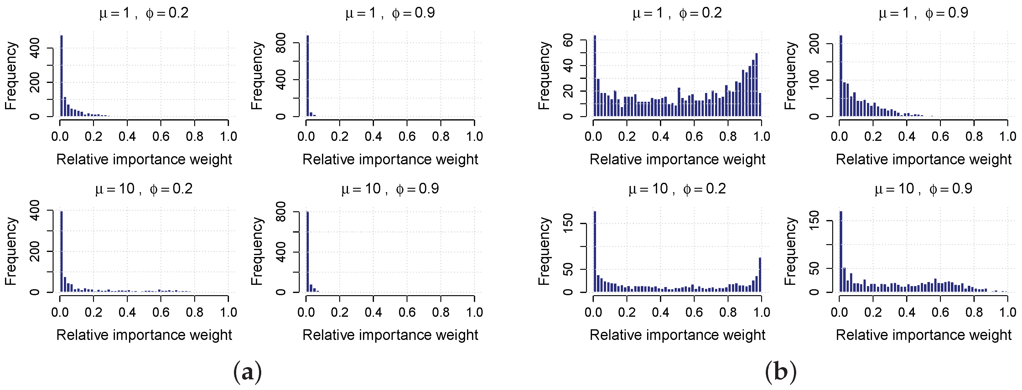
To illustrate that the same problem arises in Student-t copula models, Figure 1a displays histograms of the GHK–MVMN importance weights ${\omega }_2({\mathit{Z}}^{\left(k\right)},W^{\left(k\right)})$, normalized by their maximum, for $n=30$ and $M=1000$, across four Poisson–AR(1) t copula models with $\nu =10$. For all models, the relative weight distributions are highly concentrated near zero, indicating severe importance-weight degeneracy. For the same models, Figure 1b shows the corresponding relative weight distributions obtained using the TMET estimator based on exponential tilting, to be discussed below. TMET consistently reduces the mass of weights near zero and produces a less degenerate distribution of importance weights than GHK. This typically leads to more stable likelihood estimates, especially in low-count settings or under strong dependence. The pronounced weight degeneracy in GHK reflects a substantial mismatch between the proposal and target densities, leading to highly variable importance weights. This motivates the construction of proposal densities that explicitly control the variability of the importance weights. The minimax exponential tilting (MET) framework of [12] provides a principled construction for this purpose.

5.1. Exponential Tilting

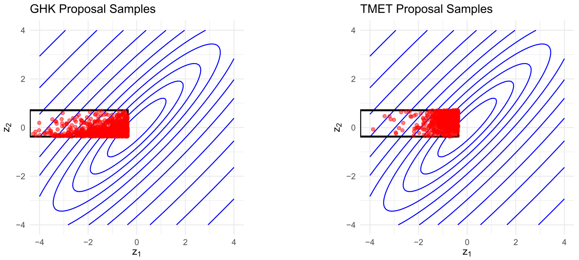
To address the severe importance weight degeneracy illustrated in Figure 1a, we modify the importance sampling density underlying the GHK–MVMN approximation through exponential tilting. Rather than sampling from $g_{\mathit{\eta },\nu }^{\left(2\right)}$, sampling is carried out from an exponentially tilted version of this density that shifts probability mass toward regions where the truncated Student-t target density is largest, thereby stabilizing the density ratios. Figure 2 provides an illustration of this goal for the t copula model with Poisson marginal with $\mu =1$, an AR$\left(1\right)$ latent process with $\varphi =0.9$ and $\nu =3$, using $n=2$, $\mathit{y}=(0,1)$ and $M=1000$. The left panel displays a sample from the GHK proposal, showing that many points fall in areas of low joint t density within the truncation set. Consequently, the corresponding density ratios ${\omega }_2({\mathit{Z}}^{\left(k\right)},W^{\left(k\right)})$ are extremely small, resulting in pronounced weight degeneracy. In contrast, the right panel displays a sample from the TMET proposal, showing that most points fall in areas of higher joint density inside the truncation region, reducing the proportion of near-zero weights relative to GHK. This example highlights the mechanism through which TMET improves importance sampling efficiency, namely, the alignment of the proposal density with the geometry of the target distribution rather than the truncation region alone.

Following [12], we focus on approximating the mixture-of-normals representation of the likelihood (16). We begin with a slight modification of the importance sampling density (24), obtained by replacing the first factor $f(w;\nu )$ with $\tilde{f}(w;\nu )$, the density of the $\mathrm{TN}(0,1;[0,\infty \left)\right)$ distribution, where $\mathrm{TN}(m,s^2;[a,b])$ denotes the $\mathrm{N}(m,s^2)$ distribution truncated to $[a,b]$. This choice places the baseline importance sampling density within an exponential family, which is essential for the minimax exponential tilting (MET) variance property discussed later. By a slight abuse of notation, we continue to write $g_{\mathit{\eta },\nu }^{\left(2\right)}(w,\mathit{z})$ for this modified density. An exponentially tilted importance sampling density then takes the form

$$g_{\mathit{\eta },\nu ,\kappa ,\mathit{\delta }}^{\left(3\right)}(w,\mathit{z})\propto g_{\mathit{\eta },\nu }^{\left(2\right)}(w,\mathit{z})exp(\kappa w+{\mathit{\delta }}^{\top }\mathit{z}),$$

where $(\kappa ,\mathit{\delta })=(\kappa ,{\delta }_1,\dots ,{\delta }_n)\in {\mathbb{R}}^{n+1}$ is a tilting vector that shifts the GHK–MVMN baseline importance sampling density, aimed toward regions where the target density is more concentrated. Since $g_{\mathit{\eta },\nu }^{\left(2\right)}(w,\mathit{z})$ is a product of univariate truncated normal densities, $g_{\mathit{\eta },\nu ,\kappa ,\mathit{\delta }}^{\left(3\right)}(w,\mathit{z})$ is also a product of exponentially tilted univariate truncated normal densities, which remain truncated normal densities [14]. Specifically,

$$g_{\mathit{\eta },\nu ,\kappa ,\mathit{\delta }}^{\left(3\right)}(w,\mathit{z})={\tilde{f}}_{\kappa }(w;\nu )q_{{\delta }_1}(z_1\mid w,y_1;\nu ,{\mathbf{\Psi }}_{\mathit{\vartheta }})\prod _{t=2}^n{q}_{{\delta }_t}(z_t\mid {\mathit{z}}_{<t},w,y_t;\nu ,{\mathbf{\Psi }}_{\mathit{\vartheta }}),$$

(31)

where

$$\begin{array}{cc}\hfill {\tilde{f}}_{\kappa }(w;\nu )& =\tilde{f}(w;\nu )exp\left(\kappa w-{\rho }_0\left(\kappa \right)\right)\hfill \\ \hfill & ={\displaystyle \frac{\varphi (w-\kappa )}{\mathrm{\Phi }\left(\kappa \right)}}{\mathbf{1}}_{(0,\infty )}\left(w\right),\hfill \end{array}$$

and, for $t=1,\dots ,n$

$$\begin{array}{cc}\hfill q_{{\delta }_t}(z_t\mid {\mathit{z}}_{<t},w,y_t;\nu ,{\mathbf{\Psi }}_{\mathit{\vartheta }})& =q(z_t\mid {\mathit{z}}_{<t},w,y_t;\nu ,{\mathbf{\Psi }}_{\mathit{\vartheta }})exp\left({\delta }_t{z}_t-{\rho }_t\left({\delta }_t\right)\right)\hfill \\ \hfill & ={\displaystyle \frac{\varphi \left({\displaystyle \frac{z_t-m_t({\mathit{z}}_{<t};\mathit{\vartheta })}{s_t\left(\mathit{\vartheta }\right)}}-s_t\left(\mathit{\vartheta }\right){\delta }_t\right)}{\mathrm{\Phi }({\tilde{b}}_t-s_t\left(\mathit{\vartheta }\right){\delta }_t)-\mathrm{\Phi }({\tilde{a}}_t-s_t\left(\mathit{\vartheta }\right){\delta }_t)}}{\mathbf{1}}_{[(w/\sqrt{\nu })a_t,(w/\sqrt{\nu })b_t]}\left(z_t\right),\hfill \end{array}$$

(32)

where ${\rho }_0\left(\kappa \right)$ and ${\rho }_t\left({\delta }_t\right)$ are the log-normalizing constants associated with the exponential tilts of $\tilde{f}(w;\nu )$ and $q(z_t\mid {\mathit{z}}_{<t},w,y_t;\nu ,{\mathbf{\Psi }}_{\mathit{\vartheta }})$, respectively, and $({\tilde{a}}_t,{\tilde{b}}_t)$ are given by

$${\tilde{a}}_t={\displaystyle \frac{(w/\sqrt{\nu })a_t-m_t({\mathit{z}}_{<t};\mathit{\vartheta })}{s_t\left(\mathit{\vartheta }\right)}}\mathrm{and}{\tilde{b}}_t={\displaystyle \frac{(w/\sqrt{\nu })b_t-m_t({\mathit{z}}_{<t};\mathit{\vartheta })}{s_t\left(\mathit{\vartheta }\right)}}.$$

(33)

Following [14], we adopt a reparameterization of the tilting parameters to simplify subsequent expressions. Inspection of (32) shows that the tilts in the Gaussian coordinates enter through the products $s_t\left(\mathit{\vartheta }\right){\delta }_t$. Since the innovation scales $s_t\left(\mathit{\vartheta }\right)$ are fixed functions of $\mathit{\vartheta }$, we define the reparameterized tilt

$${\check{\delta }}_t:=s_t\left(\mathit{\vartheta }\right){\delta }_t,t=1,\dots ,n.$$

For notational simplicity, we subsequently write ${\delta }_t$ in place of ${\check{\delta }}_t$. All expressions below are written in terms of this reparameterized tilting vector, which eliminates repeated factors of $s_t\left(\mathit{\vartheta }\right)$ and yields a more compact likelihood representation. For a fixed tilting vector $(\kappa ,\mathit{\delta })$, the approximation to the likelihood (16) based on the exponentially tilted importance sampling density (31) is given by

$$\begin{array}{cc}\hfill {\widehat{L}}^{\mathrm{ET}}(\mathit{\eta };\mathit{y})& ={\displaystyle \frac{1}{M}}\sum _{k=1}^M{\displaystyle \frac{{\varphi }_n({\mathit{Z}}^{\left(k\right)};{\mathbf{\Psi }}_{\mathit{\vartheta }})f(W^{\left(k\right)};\nu )}{g_{\mathit{\eta },\nu ,\kappa ,\mathit{\delta }}^{\left(3\right)}(W^{\left(k\right)},{\mathit{Z}}^{\left(k\right)})}}\hfill \\ \hfill & ={\displaystyle \frac{1}{M}}\sum _{k=1}^M\left[\prod _{t=1}^n{\displaystyle \frac{\mathrm{\Phi }\left({\tilde{b}}_t^{\left(k\right)}-{\delta }_t\right)-\mathrm{\Phi }\left({\tilde{a}}_t^{\left(k\right)}-{\delta }_t\right)}{exp\left(\frac{Z_t^{\left(k\right)}-m_t^{\left(k\right)}}{s_t}{\delta }_t-\frac{1}{2}{\delta }_t^2\right)}}\right]{\displaystyle \frac{2^{1-\nu /2}{\left(w^{\left(k\right)}\right)}^{\nu -1}\mathrm{\Phi }\left(\kappa \right)}{exp\left(\kappa w^{\left(k\right)}-\frac{1}{2}{\kappa }^2\right)\mathrm{\Gamma }(\nu /2)}},\hfill \end{array}$$

(34)

where $(W^{\left(1\right)},{\mathit{Z}}^{\left(1\right)}),\dots ,(W^{\left(M\right)},{\mathit{Z}}^{\left(M\right)})$ are i.i.d. draws from (31), ${\mathit{Z}}^{\left(k\right)}=(Z_1^{\left(k\right)},\dots ,Z_n^{\left(k\right)})$, ${\mathit{Z}}_{<t}^{\left(k\right)}={(Z_1^{\left(k\right)},\dots ,Z_{t-1}^{\left(k\right)})}^{\top }$, and ${\tilde{a}}_t^{\left(k\right)}$ and ${\tilde{b}}_t^{\left(k\right)}$ given in (33) are evaluated at ${\mathit{Z}}_{<t}^{\left(k\right)}$. The simulation of each of $(W^{\left(k\right)},{\mathit{Z}}^{\left(k\right)})$ is done sequentially, $W^{\left(k\right)},Z_1^{\left(k\right)},\dots ,Z_n^{\left(k\right)}$, using any algorithm to simulate from truncated normal distributions.

The efficiency of the importance sampling estimator (34) depends on two factors. First, the conditional moments $m_t({\mathit{z}}_{<t};\mathit{\vartheta })$ and $s_t^2\left(\mathit{\vartheta }\right)$ need to be computed efficiently, which is carried out using the Innovations algorithm discussed in Section 4.2. These tasks involve $O\left(n\right)$ complexity, much faster than computing them using the Cholesky decomposition of ${\mathbf{\Psi }}_{\mathit{\vartheta }}$, which involves $O\left(n^3\right)$ complexity. Second, the tilting vector $(\kappa ,\mathit{\delta })$ needs to be chosen judiciously so the samples from (31) are mostly in the high-density region of the target density. This makes the variance of the density ratio smaller and produces an estimator with improved efficiency relative to the estimator (26).

5.2. Minimax Exponential Tilting

Here we describe how to choose the tilting vector $(\kappa ,\mathit{\delta })$ in a manner that is computationally efficient and tailored to the time series setting, where the latent process is a t–ARMA process. Following [12,32], the tilting vector is chosen to minimize the worst-case density ratio (importance weight) over the truncation region, thereby reducing the risk of weight degeneracy, that is, situations in which a few samples dominate the estimator and inflate its variance. Define the log-importance weight function associated with the estimator (34) by

$$\begin{array}{cc}\hfill \psi (w,\mathit{z},\kappa ,\mathit{\delta })& =log\left({\displaystyle \frac{{\varphi }_n(\mathit{z};{\mathbf{\Psi }}_{\mathit{\vartheta }})f(w;\nu )}{g_{\mathit{\eta },\nu ,\kappa ,\mathit{\delta }}^{\left(3\right)}(w,\mathit{z})}}\right)\hfill \\ & =-{(\mathit{z}-\mathit{B}\mathit{z})}^{\top }{\mathit{D}}^{-1}\mathit{\delta }+\frac{1}{2}{\parallel \mathit{\delta }\parallel }^2+\sum _{t=1}^{n}log\left[\mathrm{\Phi }({\tilde{b}}_t-{\delta }_t)-\mathrm{\Phi }({\tilde{a}}_t-{\delta }_t)\right]\hfill \\ \hfill & -\kappa w+\frac{1}{2}{\kappa }^2+log\mathrm{\Phi }\left(\kappa \right)+(\nu -1)logw+c,\hfill \end{array}$$

where $\mathit{D}=\mathrm{diag}(s_1,\dots ,s_n)$ contains the one-step predictive standard deviations, $\mathit{B}=\left(b_{ij}\right)$ is the $n\times n$ lower-triangular matrix of best linear predictor (BLP) coefficients defined below, and ${\tilde{a}}_t,{\tilde{b}}_t$ are given in (33); c collects the terms that do not depend on the tilting vector. Throughout the discussion below, $(\mathit{y},\mathit{\eta })$ are treated as fixed. Following [12], the optimal tilting vector is defined as the solution to the convex–concave saddle-point problem

$$\underset{(\kappa ,\mathit{\delta })\in {\mathbb{R}}^{n+1}}{inf}\underset{(w,\mathit{z})\in [0,\infty )\times [\mathit{a},\mathit{b}]}{sup}\psi (w,\mathit{z},\kappa ,\mathit{\delta }).$$

(35)

The next result, proved in Appendix A, states that $\psi (·)$ is concave in $(w,\mathit{z})$ and convex in $(\kappa ,\mathit{\delta })$, ensuring a unique saddle point.

Theorem 1.

For $\nu >2$, the problem (35) admits a unique solution $(w^{*},{\mathit{z}}^{*},{\kappa }^{*},{\mathit{\delta }}^{*})$, with $(w^{*},{\mathit{z}}^{*})\in [0,\infty )\times [\mathit{a},\mathit{b}]$, satisfying

$${\displaystyle \frac{\partial \psi }{\partial \mathit{\delta }}}(w^{*},{\mathit{z}}^{*},{\kappa }^{*},{\mathit{\delta }}^{*})=\mathbf{0},{\displaystyle \frac{\partial \psi }{\partial \kappa }}(w^{*},{\mathit{z}}^{*},{\kappa }^{*},{\mathit{\delta }}^{*})=0.$$

For solving (35) and evaluating (34), substantial simplifications arise when the latent process is a causal and invertible t–ARMA$(p,q)$ process, for some $p,q\ge 0$. In this setting, the conditional moments $(m_t,s_t^2)$ can be computed in linear time using the Innovations algorithm described in Section 4.2. More importantly for the proposed implementation, the correlation structure of causal and invertible t–ARMA processes implies that the associated best linear prediction (BLP) matrix $\mathit{B}$ is sparse. When the latent process is a t–ARMA process, the likelihood approximation (34) with tilting vector $(w^{*},{\mathit{z}}^{*},{\kappa }^{*},{\mathit{\delta }}^{*})$ is called the TMET method.

For pure AR$\left(p\right)$ processes, the BLP matrix $\mathit{B}$ is strictly lower triangular with bandwidth p. Specifically, for $t<p$, the BLP coefficients ${\mathit{b}}_t^{\top }$ are obtained from the Durbin–Levinson recursions [23], Section 5.3, while for $t\ge p$ they coincide with the autoregressive parameters, with exactly p nonzero entries located at positions $t-p,\dots ,t-1$

$${\mathit{b}}_t^{\top }=\left\{\begin{array}{cc}(b_{t1},\dots ,b_{t,t-1},0,\dots ,0),\hfill & t<p,\hfill \\ (0,\dots ,0,{\varphi }_1,\dots ,{\varphi }_p,0,\dots ,0),\hfill & t\ge p.\hfill \end{array}\right.$$

(36)

As a result, $\mathit{B}$ has $O\left(np\right)$ nonzero entries.

For invertible ARMA$(p,q)$ processes, we adopt the standard infinite-order autoregressive representation

$$Z_t=\sum _{j=1}^{\infty }{\pi }_j{Z}_{t-j}+{ϵ}_t,t\in \mathbb{Z},$$

where $\left\{{ϵ}_t\right\}$ denotes the zero-mean Gaussian white-noise innovation process appearing in the ARMA difference Equation (7), and the coefficients $\left\{{\pi }_j\right\}$ decay exponentially fast under causality and invertibility; see [23], Section 3.1.

Following [14], we truncate this representation after $p^{\prime }$ terms, yielding a practically accurate finite-order approximation because of the rapid decay of the coefficients ${\pi }_j$. The truncated process is then treated as an AR$\left(p^{\prime }\right)$ process, and the construction above applies. In particular, for $t\ge p^{\prime }$, the BLP coefficients take the form

$${\mathit{b}}_t^{\top }=(0,\dots ,0,{\pi }_1,\dots ,{\pi }_{p^{\prime }},0,\dots ,0),$$

resulting in a banded BLP matrix $\mathit{B}$ with $O\left(n{p}^{\prime }\right)$ nonzero entries. The truncation order $p^{\prime }$ controls the sparsity of the matrix $\mathit{B}$ and thus the computational cost of computing the tilting parameters in TMET, but does not affect the target likelihood. Under causality and invertibility, the autoregressive coefficients decay exponentially fast, so moderate values of $p^{\prime }$ yield accurate finite-order approximations in practice. We use $p^{\prime }=30$ as a default choice, which provides stable likelihood approximations and parameter estimates across all settings considered; see [14]. Consequently, matrix-vector products involving $\mathit{B}$ or ${\mathit{B}}^{\top }$ can be computed in $O\left(n\right)$ time, and all Hessian-vector products required by the optimization algorithm introduced below inherit this linear complexity.

5.3. Solving the Saddle-Point Problem

A direct solution of (35) using the trust-region Newton method of [12] requires the inversion of dense $2n\times 2n$ Hessian matrices and repeated Cholesky factorizations to compute the conditional moments $(m_t,s_t^2)$, resulting in an $O\left(n^3\right)$ computational cost. This is computationally prohibitive for time series of moderate to large length. Rather than solving the saddle-point problem (35) directly, we compute the optimal tilting vector by minimizing the squared gradient norm

$$Q(w,\mathit{z},\kappa ,\mathit{\delta }):=\frac{1}{2}{∥\nabla \psi (w,\mathit{z},\kappa ,\mathit{\delta })∥}_2^2.$$

This defines a nonlinear least-squares problem whose global minimizers satisfy the stationarity conditions $\nabla \psi (w,\mathit{z},\kappa ,\mathit{\delta })=\mathbf{0}$. We minimize Q using a Levenberg–Marquardt (LM) iteration. Let ${\mathit{x}}^{\left(r\right)}=(w^{\left(r\right)},{\mathit{z}}^{\left(r\right)},{\kappa }^{\left(r\right)},{\mathit{\delta }}^{\left(r\right)})$ denote the current iterate, and define ${\mathbf{g}}_{\psi }^{\left(r\right)}:=\nabla \psi \left({\mathit{x}}^{\left(r\right)}\right)$ and ${\mathbf{H}}_{\psi }^{\left(r\right)}:={\nabla }^2\psi \left({\mathit{x}}^{\left(r\right)}\right)$ as the gradient and Hessian of $\psi (·)$ evaluated at ${\mathit{x}}^{\left(r\right)}$. At iteration r, the LM search direction $\mathrm{\Delta }{\mathit{x}}^{\left(r\right)}$ is obtained from the damped normal equations

$$\left({\mathbf{H}}_{\psi }^{\left(r\right)\top }{\mathbf{H}}_{\psi }^{\left(r\right)}+{\lambda }^{\left(r\right)}\mathbf{I}\right)\mathrm{\Delta }{\mathit{x}}^{\left(r\right)}=-{\mathbf{H}}_{\psi }^{\left(r\right)\top }{\mathbf{g}}_{\psi }^{\left(r\right)},$$

(37)

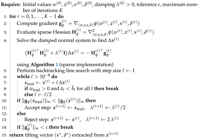
where ${\lambda }^{\left(r\right)}>0$ is an adaptive damping parameter that provides regularization and improves numerical stability in the presence of heavy tails and strong dependence [33]. The update direction $\mathrm{\Delta }{\mathit{x}}^{\left(r\right)}$ is computed by solving (37) using a preconditioned conjugate-gradient (PCG) method [34], Section 11.5.2. PCG is employed solely as a linear solver, allowing $\mathrm{\Delta }{\mathit{x}}^{\left(r\right)}$ to be computed efficiently without forming or factorizing the dense matrix ${\mathbf{H}}_{\psi }^{\left(r\right)\top }{\mathbf{H}}_{\psi }^{\left(r\right)}$. The new iterate is then given by

$${\mathit{x}}^{(r+1)}={\mathit{x}}^{\left(r\right)}+l\mathrm{\Delta }{\mathit{x}}^{\left(r\right)},$$

where the step size l is determined by a backtracking line search that enforces feasibility constraints, such as $w>0$ and ${\tilde{a}}_t<{\tilde{b}}_t$. The preconditioner reduces the condition number of the matrix in the damped normal equations, thereby accelerating convergence of the conjugate-gradient iterations.

All matrix-vector operations involve only the banded matrices $\mathit{B}$ and $\mathit{D}$, so each LM–PCG iteration takes $O\left(n\right)$ operations. Closed-form expressions for the gradient vector and Hessian matrix are given in Proposition A1, and their derivations are provided in Appendix A. Algorithms 1 and 2 summarize the complete implementation. Since each LM–PCG step takes $O\left(n\right)$ operations, and the number of Levenberg–Marquardt iterations remains moderate in practice, the overall computational cost of TMET grows approximately linearly with the series length. This reduces the computational cost of MET from cubic to near-linear. To our knowledge, the TMET method is the first implementation that makes MET computationally feasible for long time series, enabling likelihood-based inference for Student-t copula count models at scales that were previously impractical.

Algorithm 1 Preconditioned Conjugate Gradient (PCG) Solver

Algorithm 2 Levenberg–Marquardt Optimization for Tilting Vector $(\kappa ,\mathit{\delta })$

Although the TMET algorithm largely follows the structure of its Gaussian counterpart developed in [14], the Student-t copula setting introduces additional steps associated with the scale-mixture representation, including simulation of the latent mixing variable and modified importance weights, which makes solving the saddle-point problem more challenging. For completeness and reproducibility, Algorithm 3 summarizes the full TMET implementation specialized to the t copula model.

Algorithm 3 TMET Likelihood Approximation for t Copula Count Time Series

Remark 5.

The TMET method is not directly applicable to improve the GHK–MVT likelihood approximation, because exponential tilting does not preserve a tractable exponential-family structure for truncated t distributions, which is essential for the convex minimax optimization underlying TMET. For the t copula model, the scale variable W induces heavier tails and stronger time dependence, leading to ill-conditioned Hessian matrices that hinder gradient-based Newton-type optimization. This motivated the LM–PCG strategy adopted in this work.

Remark 6.

The importance weights (38) in Algorithm 3 are products of a large number of probabilities and can therefore become extremely small for moderate or large n. To avoid numerical underflow or loss of precision, all weights are evaluated on the log scale and combined using standard log–sum–exp stabilization. We follow the implementation strategy described in [14].

6. Simulation Study

We simulate count time series ${\left\{Y_t\right\}}_{t=1}^n$ from the model (12), with marginal cdfs $\left\{F_t(·;\mathit{\psi })\right\}$ and $\left\{V_t\right\}$ a t–ARMA$(p,q)$ process with $\nu$ degrees of freedom as defined in Section 2.2, using the following steps:

1.

Set ${\sigma }^2$ to the value in (13).

2.

Simulate $\left\{Z_t\right\}$ from the Gaussian ARMA$(p,q)$ process (7), and simulate $W\sim {\chi }_{\nu }$ independently of $\left\{Z_t\right\}$.

3.

Set

$$V_t={\displaystyle \frac{Z_t}{W/\sqrt{\nu }}},t=1,\dots ,n.$$

4.

Set

$$Y_t=F_t^{-1}\left(T(V_t;\nu );\mathit{\psi }\right),t=1,\dots ,n.$$

6.1. Simulation Setup

We conduct a simulation study to evaluate the accuracy, stability, and computational efficiency of the CE, GHK–MVMN, GHK–MVT, and TMET approximations to the likelihoods of Student-t copula time series models. Datasets were simulated from models with a wide range of marginal and dependence structures. The marginal distributions were Poisson with mean $\mu \in \{1,10\}$, chosen to represent high and moderate degrees of discreteness. The latent processes were t–ARMA processes described in Section 2.2, with a broad range of dependence strengths and tail behaviors. We considered three latent structures: AR(1), MA(1), and ARMA(1,1) processes. For AR(1) and MA(1) processes, the dependence parameter took values in $\{-0.8,-0.2,0.2,0.8\}$, representing weak and strong dependence in both positive and negative directions. For ARMA(1,1) processes, the dependence parameters took values $(\varphi ,\theta )\in \left\{\right(0.2,0.2),(0.2,0.8),(0.8,0.2),(0.8,0.8\left)\right\}$, covering both weak and strong dependence. Finally, we considered two degrees-of-freedom values, $\nu \in \{3,10\}$, representing heavy and moderately heavy tails. For likelihood approximation accuracy (see below), we generated 200 independent replications of time series of length $n=1500$, which is the largest sample size for which the MET implementation in the TruncatedNormal package is computationally feasible. To assess the finite-sample behavior of the maximum likelihood estimators (see below), we generated 100 Monte Carlo replications with sample size $n=5000$.

All simulation-based likelihood approximations (GHK–MVMN, GHK–MVT, and TMET) were computed using randomized quasi-Monte Carlo (QMC) sampling based on the irrational additive lattice (Weyl) rule with a Cranley–Patterson shift. QMC is particularly effective in this setting because the sequential conditioning in both GHK and TMET approximations induces low effective dimension, leading to substantially lower Monte Carlo variance than pseudo-random sampling. Each likelihood evaluation used $M=1000$ QMC samples, which provides a stable balance between variance reduction and computational cost. To ensure a fair comparison, the same QMC configuration (sample size, randomization, and generating vector) was used for all simulation-based estimators. The QMC implementation is identical to that used by [14] for the TMET method in Gaussian copula models. The CE approximation is fully deterministic and therefore involves no Monte Carlo sampling. The approximate likelihoods were maximized using the BFGS routine in optim, where the marginal parameters were initialized using canonical Poisson GLM fits, and the dependence parameters were initialized from ARMA fits to the observed counts. All methods were implemented in the gctsc R package developed by the authors. Computationally intensive components, including recursive conditional moment evaluation via the Innovations algorithm and simulation from truncated distributions, are implemented within the package in C++ using the R package Rcpp for efficiency.

We assess the performance of the competing likelihood approximations along three dimensions: likelihood approximation accuracy, computational efficiency, and the sampling distributions of maximum likelihood estimators (MLEs). First, likelihood approximation accuracy is evaluated using the relative error

$$\mathrm{RelErr}:={\displaystyle \frac{{\widehat{\ell }}_{\mathrm{approx}}-{\widehat{\ell }}_{\mathrm{MET}}}{|{\widehat{\ell }}_{\mathrm{MET}}|}},$$

(39)

where ${\widehat{\ell }}_{\mathrm{approx}}$ denotes the log-likelihood obtained from a given approximation, and ${\widehat{\ell }}_{\mathrm{MET}}$ is the MET log-likelihood approximation of [12]. The latter serves as a high-accuracy benchmark, but incurs an $O\left(n^3\right)$ computational cost. Second, computational efficiency is assessed by comparing the wall-clock time required for a single likelihood evaluation across methods. For each replication, runtimes are normalized by the corresponding MET runtime obtained using TruncatedNormal under identical computing conditions, and the resulting ratios are summarized across replications. Third, the sampling distributions of the MLEs obtained from the likelihood approximations are graphically compared.

6.2. Results

Given the large number of simulation scenarios considered, the complete set of figures is reported in Appendix B to keep the main text focused on the principal findings.

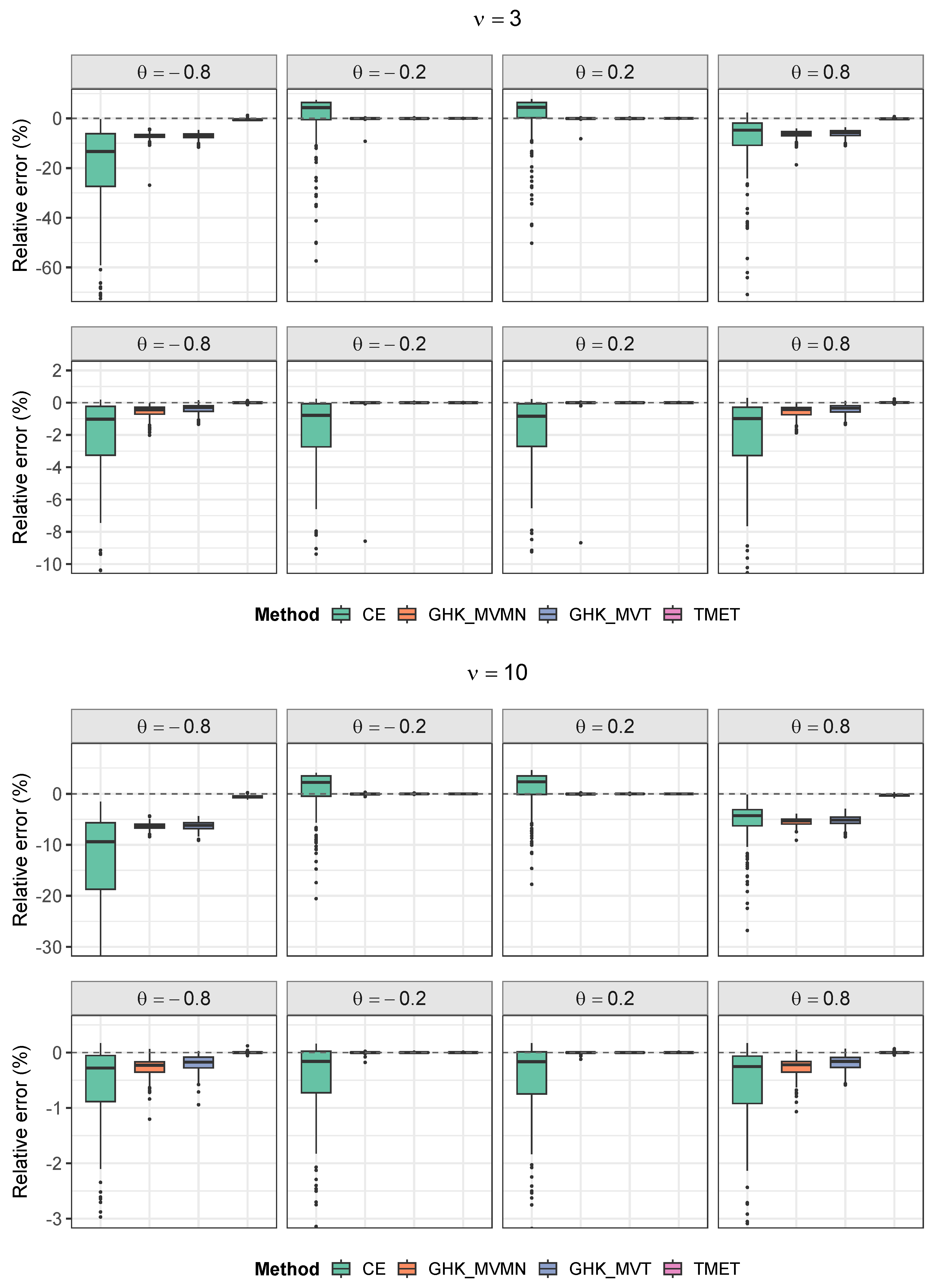
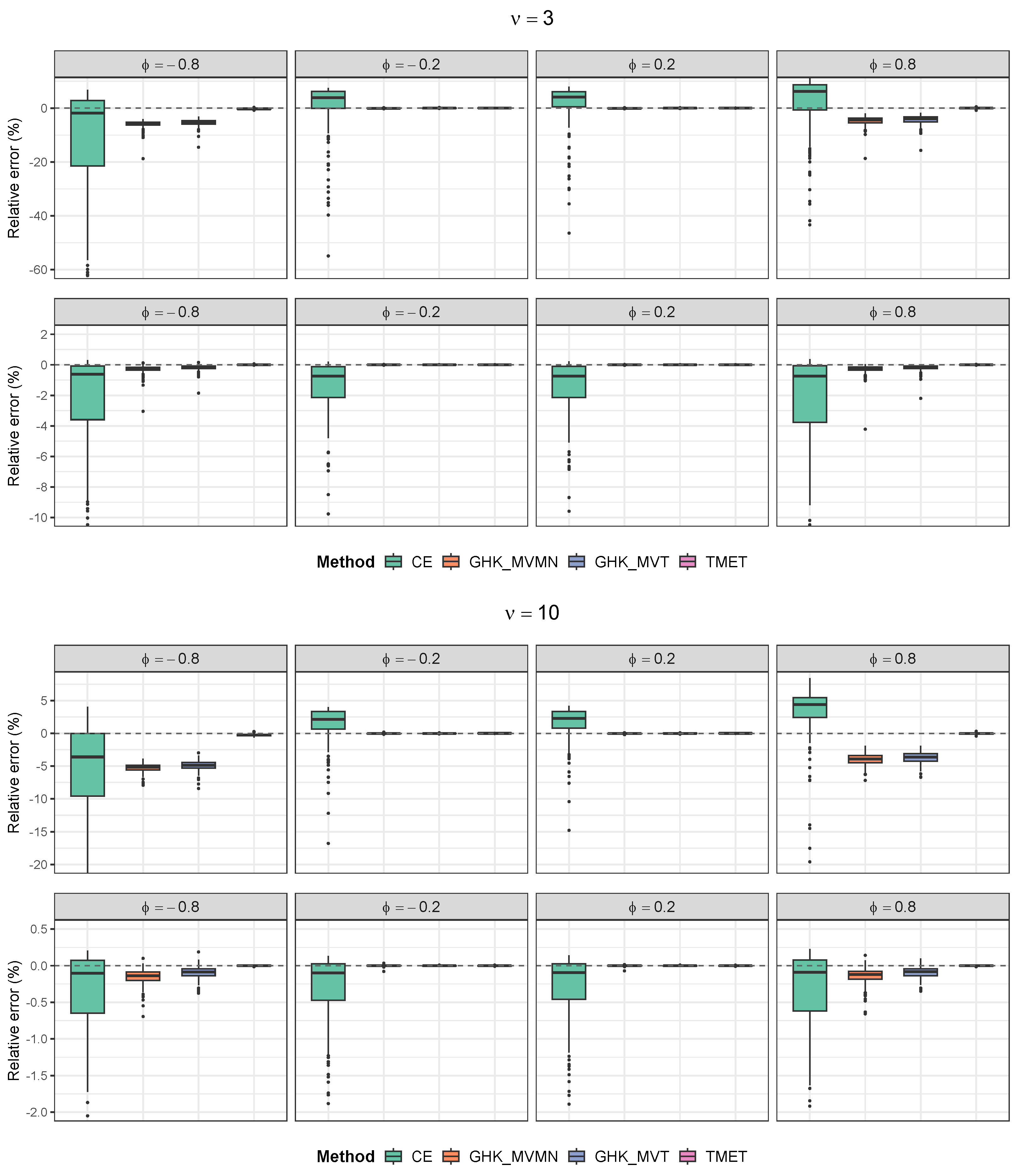
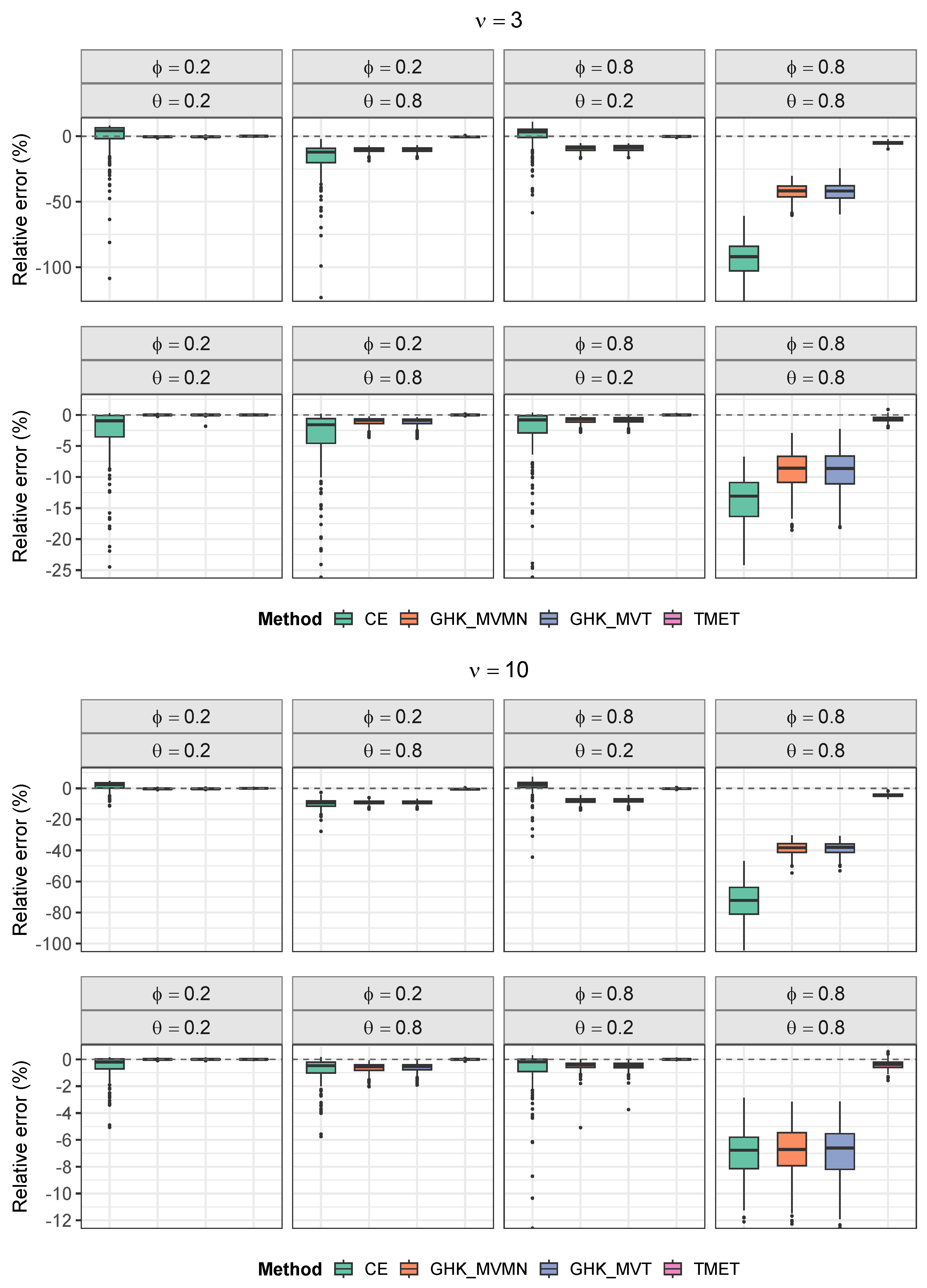
Likelihood Accuracy. Figure A1, Figure A2 and Figure A3 report the relative error (39) of each likelihood approximation for models with, respectively, AR(1), MA(1), and ARMA(1,1) latent processes. Across all scenarios, the TMET and MET approximations are essentially indistinguishable, and relative errors remain close to zero even in the most challenging models, particularly those with $\mu =1$, $\nu =3$, and strong serial dependence. TMET differs from MET only in its computational implementation, as it exploits the sequential conditional representation induced by the latent ARMA structure and the resulting sparsity to avoid dense matrix operations and Cholesky decompositions. Consequently, TMET targets the same optimally tilted importance sampler as MET, but with near-linear computational complexity in the series length.

In contrast, both GHK–MVMN and GHK–MVT often underestimate the log-likelihood. This negative bias increases as serial dependence strengthens or the degree of discretization increases, and is most pronounced for $\nu =3$. This behavior is especially severe for ARMA(1,1) latent processes with large values of $\left|\varphi \right|$ or $\left|\theta \right|$, which induce stronger and more persistent conditional dependence than AR(1) or MA(1) models and substantially complicate sequential importance sampling. This behavior is consistent with the findings of [12], who showed that Genz-type sequential estimators exhibit large variance and substantial relative error under strong dependence or severe truncation. The GHK approximations considered here belong to the same class of sequential conditional importance samplers and display analogous instability in copula-based time series settings with heavy tails and strong serial dependence.

The CE approximation displays relatively good performance when the mean is moderate ($\mu =10$) and serial dependence is weak, but its bias increases substantially under strong discretization ($\mu =1$) or heavy tails ($\nu =3$). This mirrors earlier findings for Gaussian copula models [31], where smooth discrete truncation leads to underestimation of probability mass in narrow truncation regions.

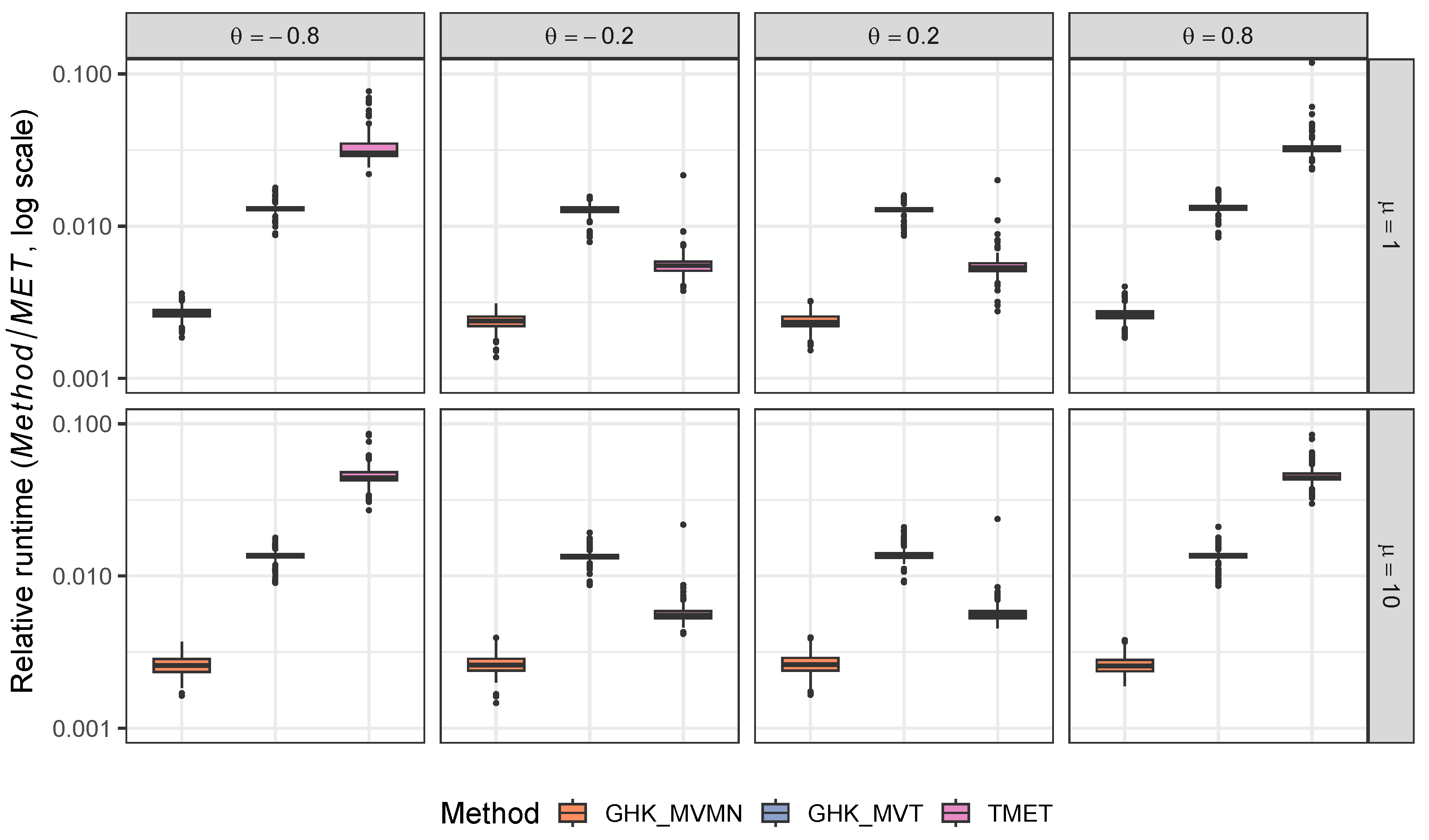
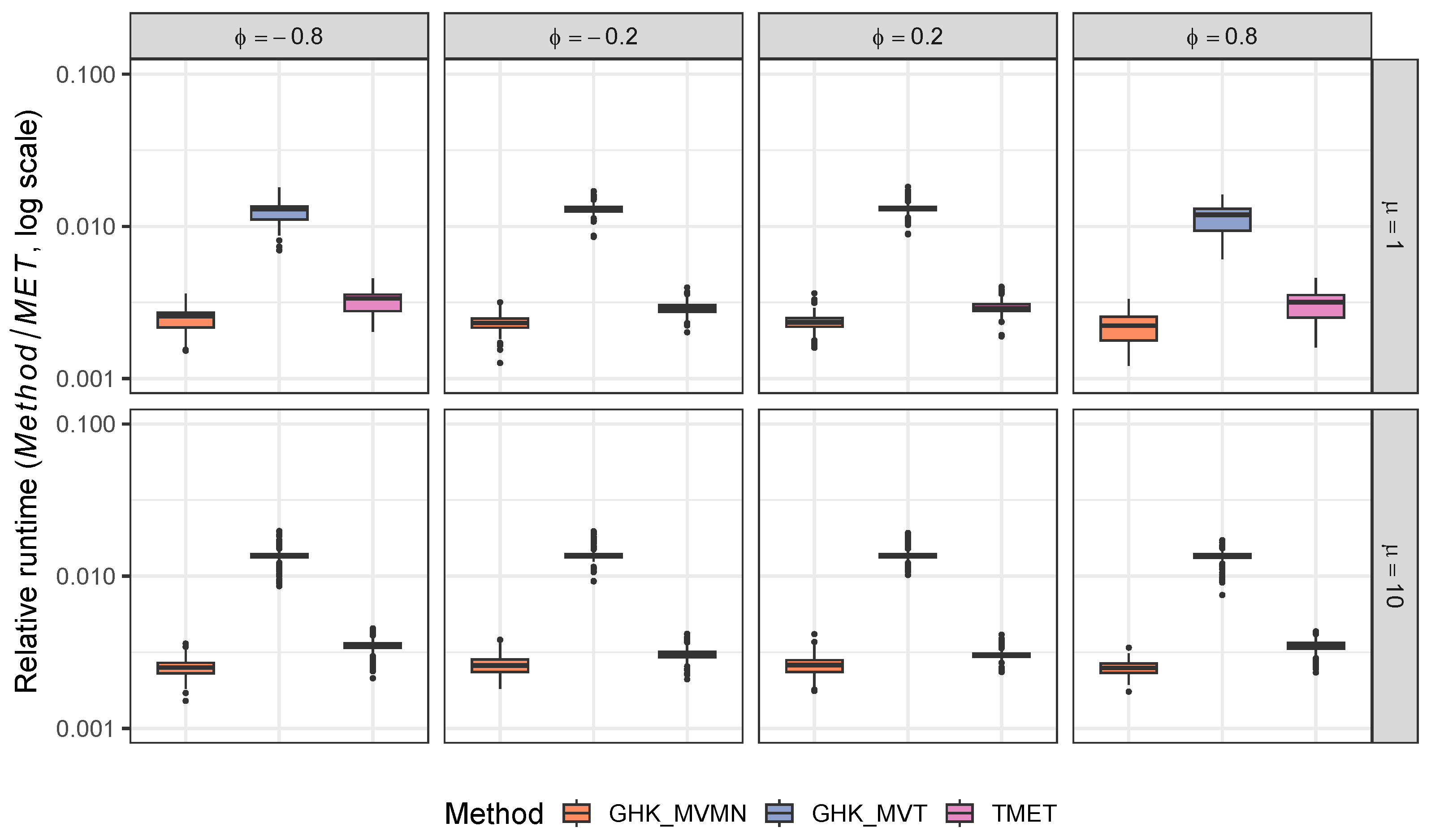
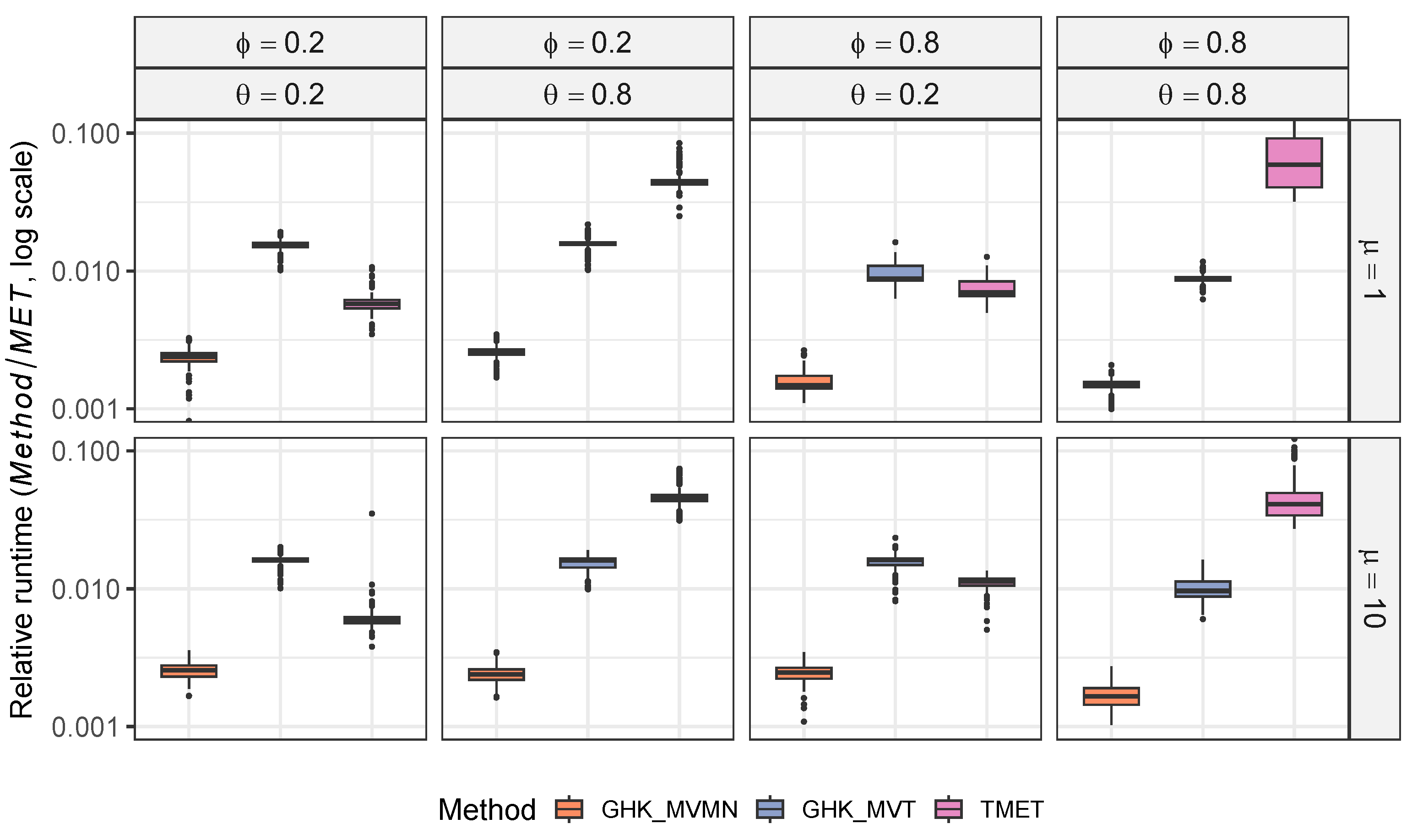
Computational Efficiency. Figure A4, Figure A5 and Figure A6 report the computation times of the simulation-based likelihood approximations relative to the MET approximation for models with, respectively, AR(1), MA(1), and ARMA(1,1) latent processes. The deterministic CE approximation, which requires only a single evaluation of the Innovations algorithm and has $O\left(n\right)$ computational complexity, is typically more than two orders of magnitude faster than the simulation-based approximations, so it is omitted from the time comparisons. Both GHK variants have $O\left(Mnm\right)$ computational complexity, since each Monte Carlo replication requires a full-length n sequential conditional recursion, where M is the number of Monte Carlo samples and $m=max\{p,q\}$, with p and q denoting the AR and MA orders. GHK–MVMN is consistently faster than GHK–MVT, reflecting the lower cost of simulating from truncated normal distributions and evaluating $\mathrm{\Phi }(·)$, relative to simulating from truncated t distributions and evaluating $T(·)$. The TMET approximation has the same $O\left(Mnm\right)$ Monte Carlo cost as GHK–MVMN, plus an additional $O\left(Tn{p}^{\prime }\right)$ cost for computing the tilting parameters, where T denotes the number of Levenberg–Marquardt iterations and $p^{\prime }$ is the truncation order used to approximate the infinite-order autoregressive representation. This additional cost arises from the Levenberg–Marquardt optimization and associated preconditioned conjugate-gradient iterations, but remains modest in practice. TMET runs particularly rapidly for AR(1) latent processes, but more slowly for MA(1) and ARMA(1,1) latent processes. The more complex conditional dependence and reduced sparsity of the latter result in the computation of the tilting vector requiring more iterations. This additional runtime is more noticeable when serial dependence is strong, but remains small relative to the $O\left(n^3\right)$ complexity of the MET benchmark.

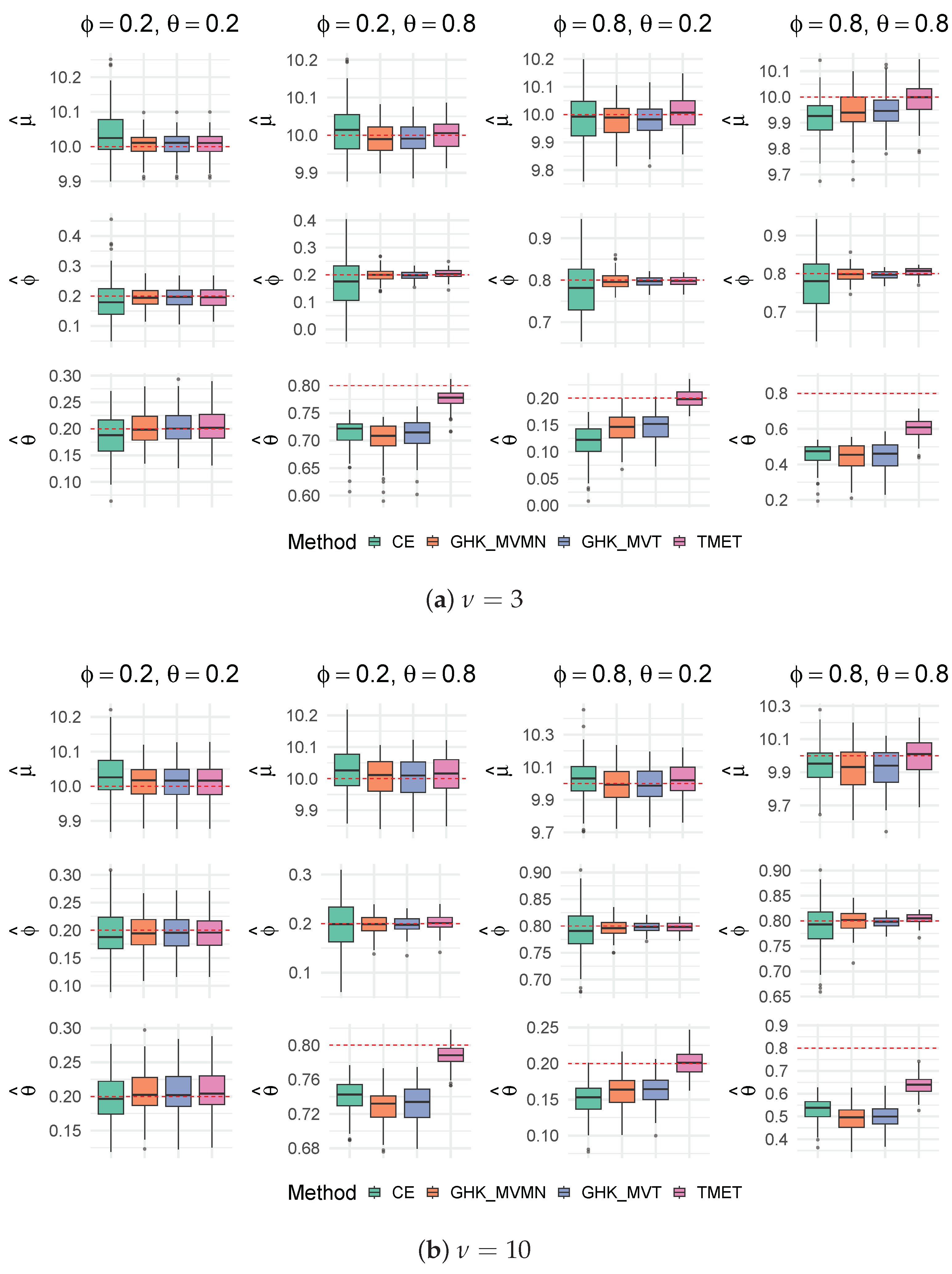
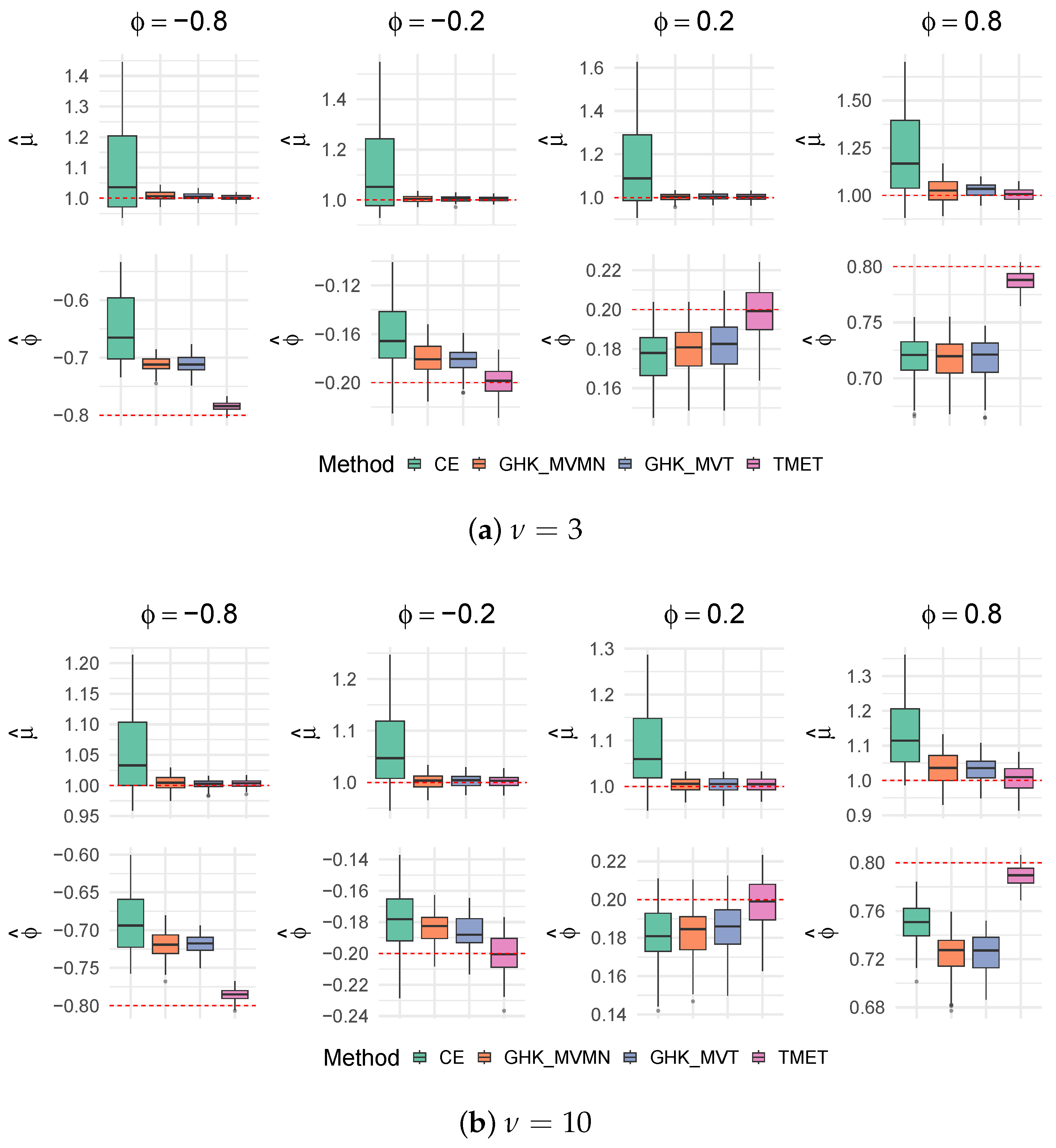
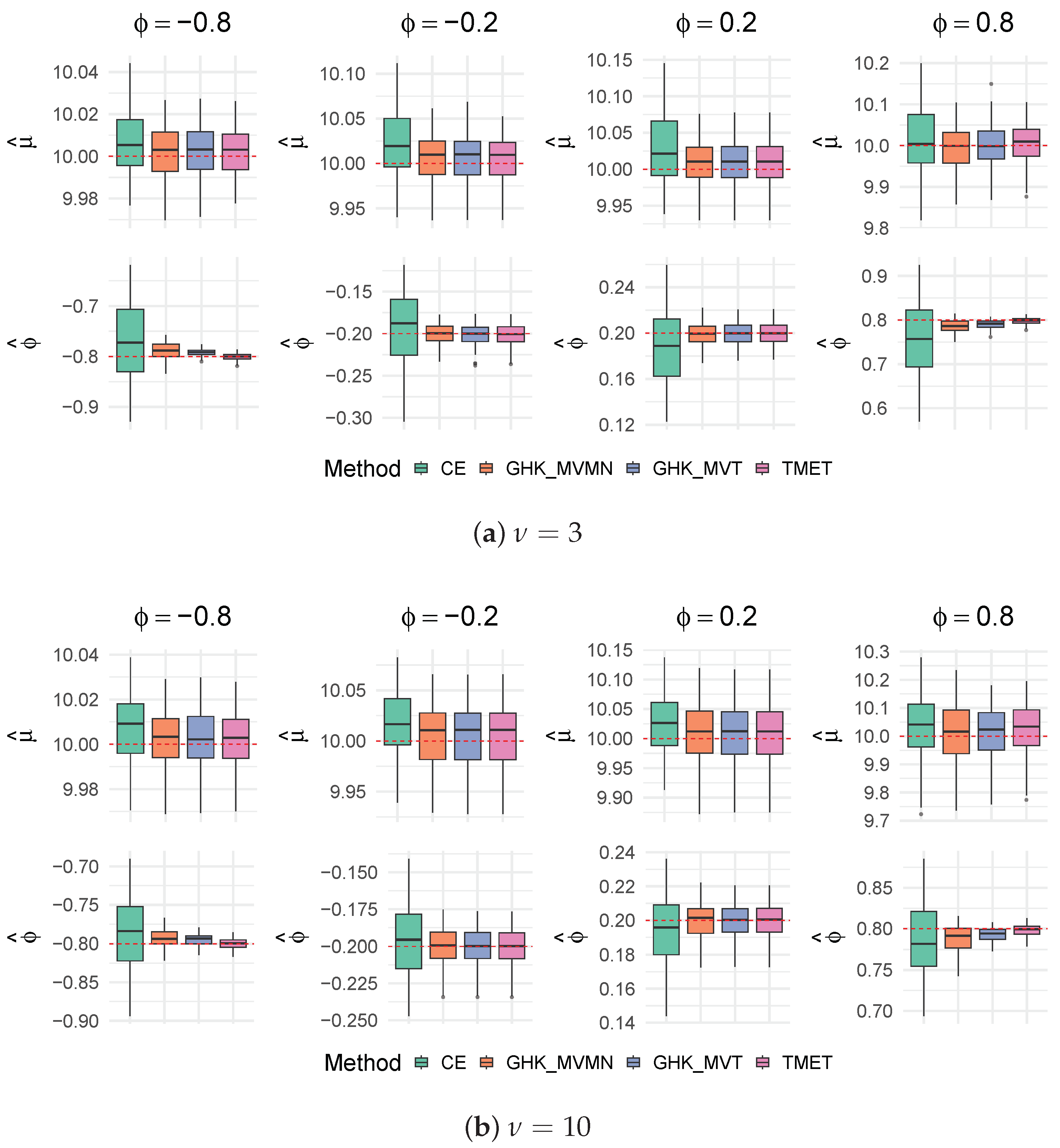
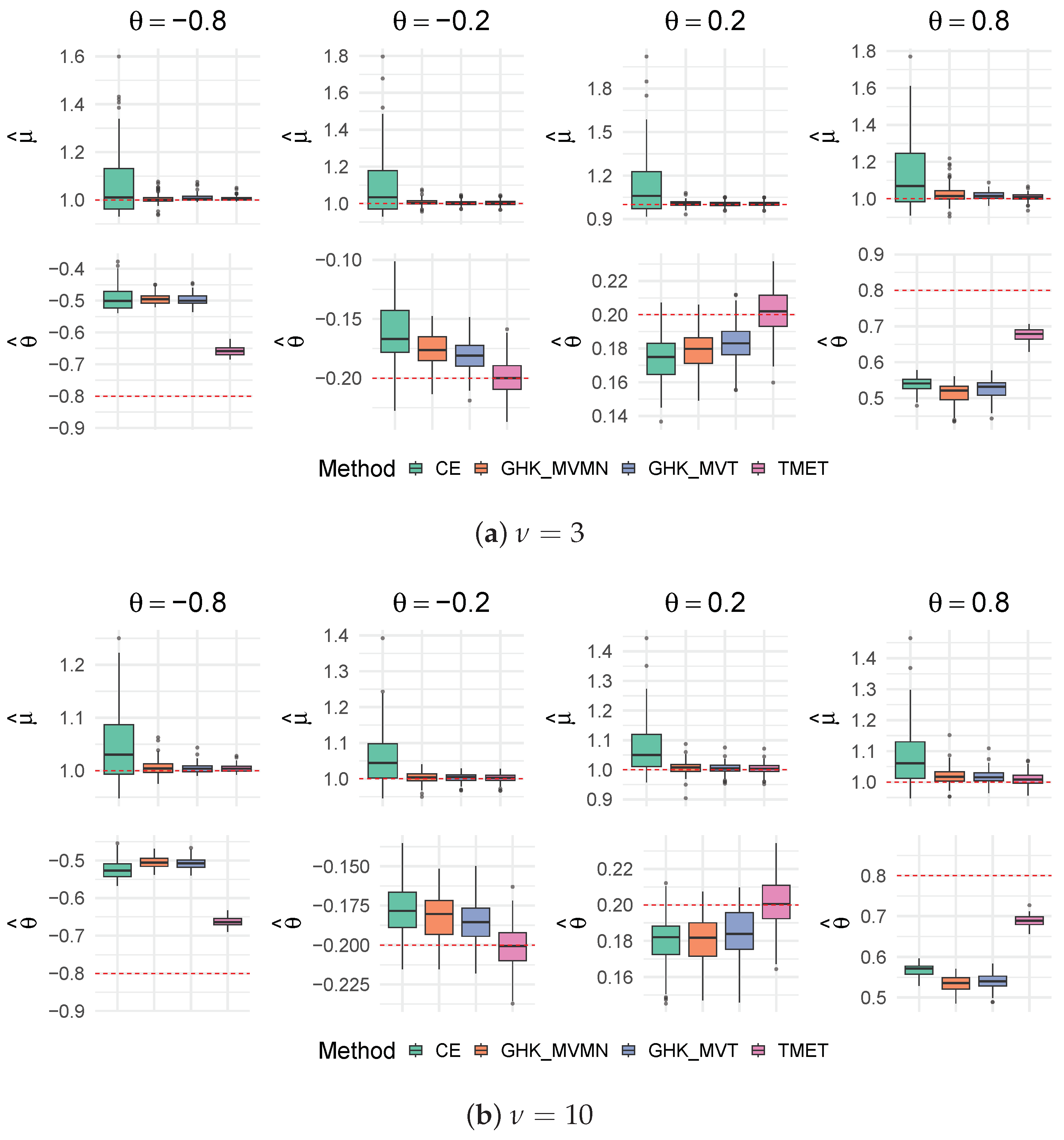
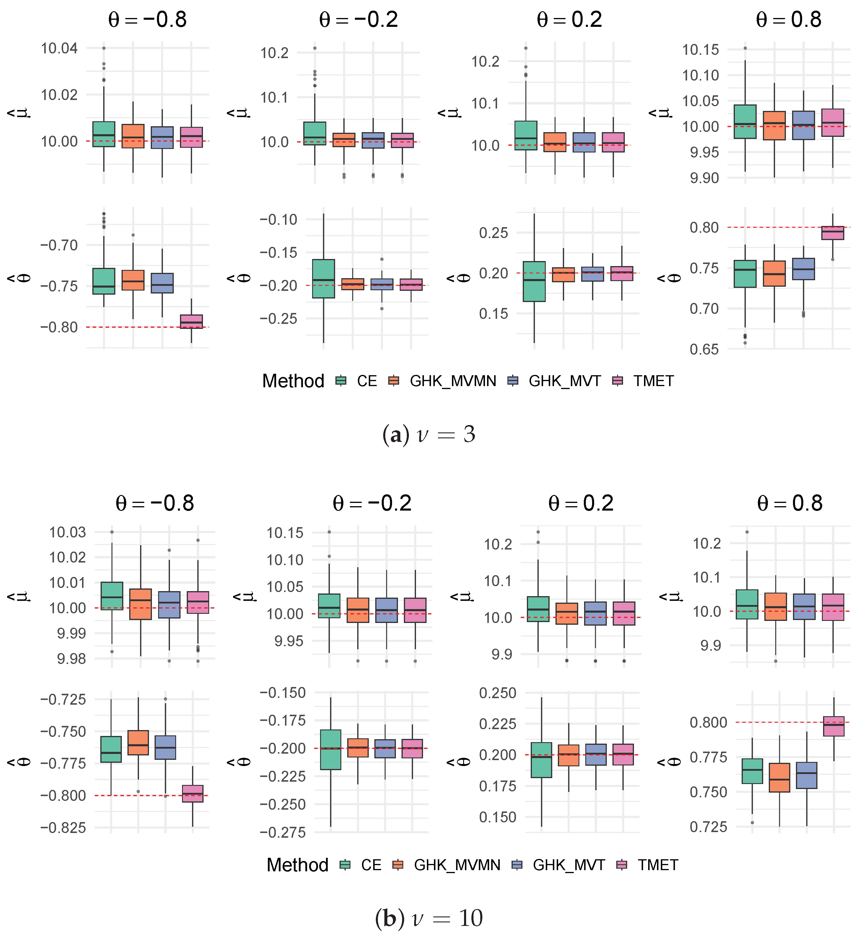
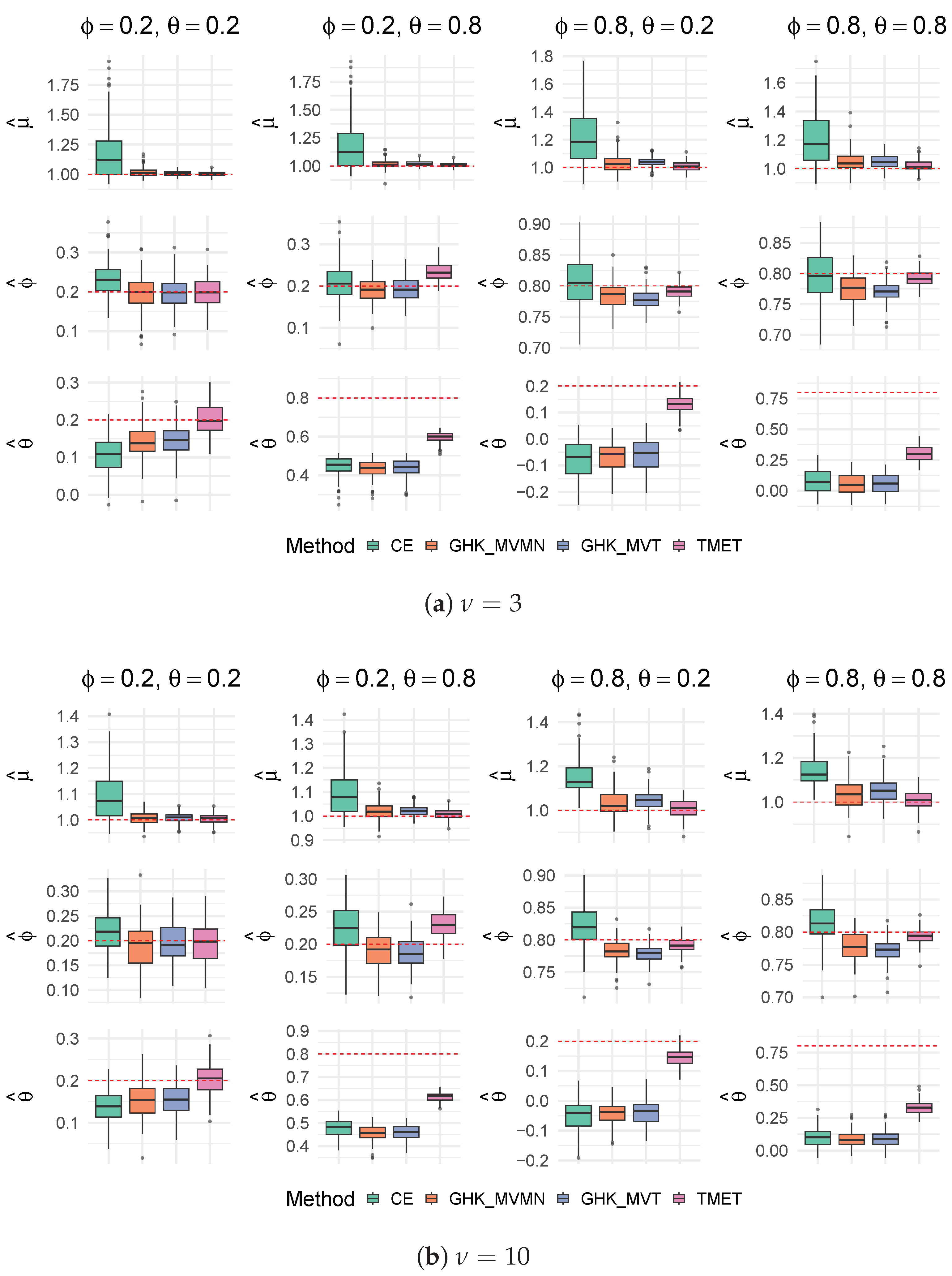
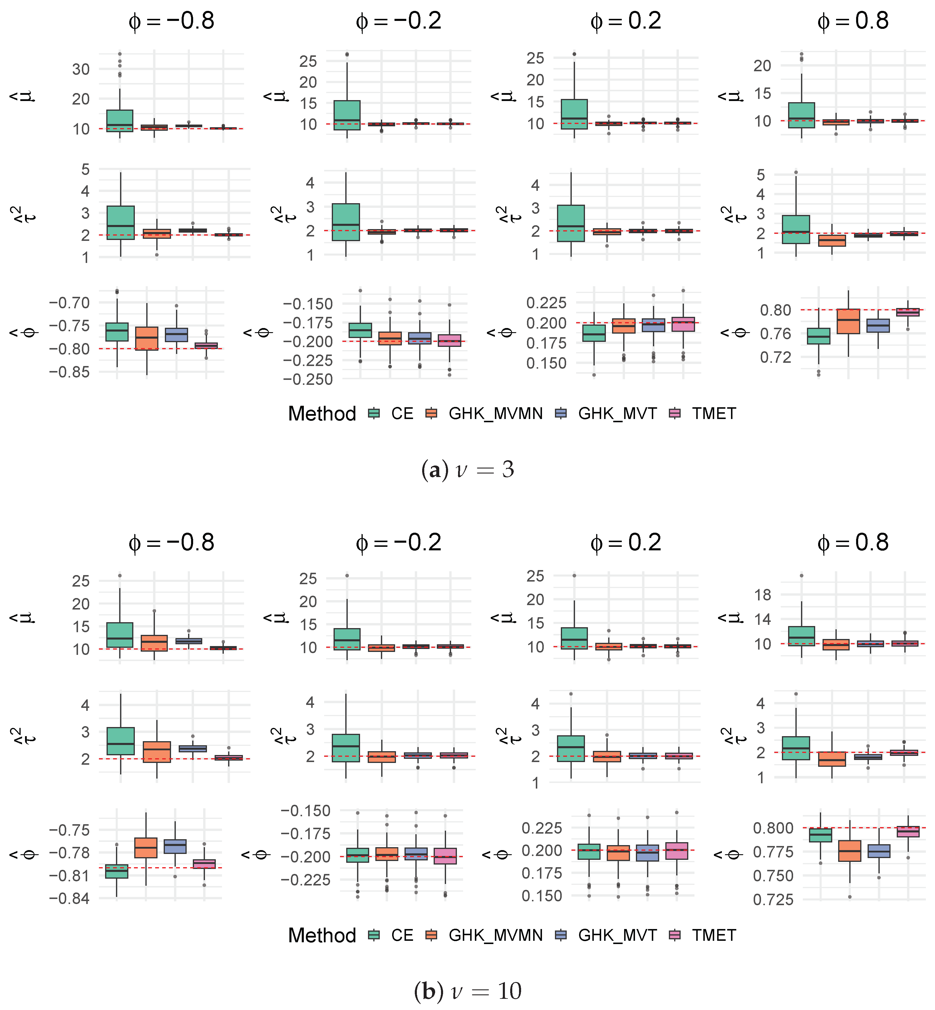
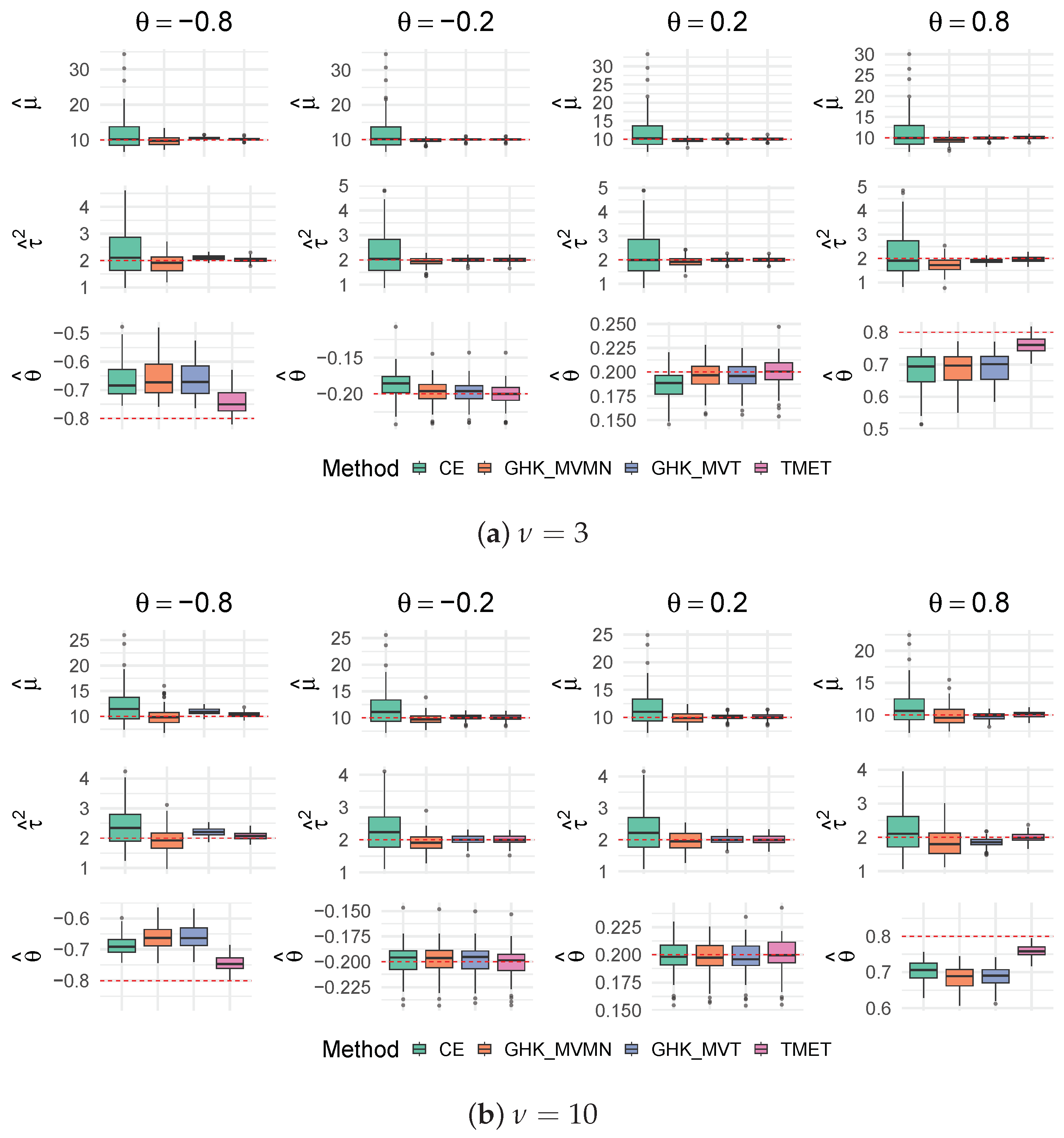
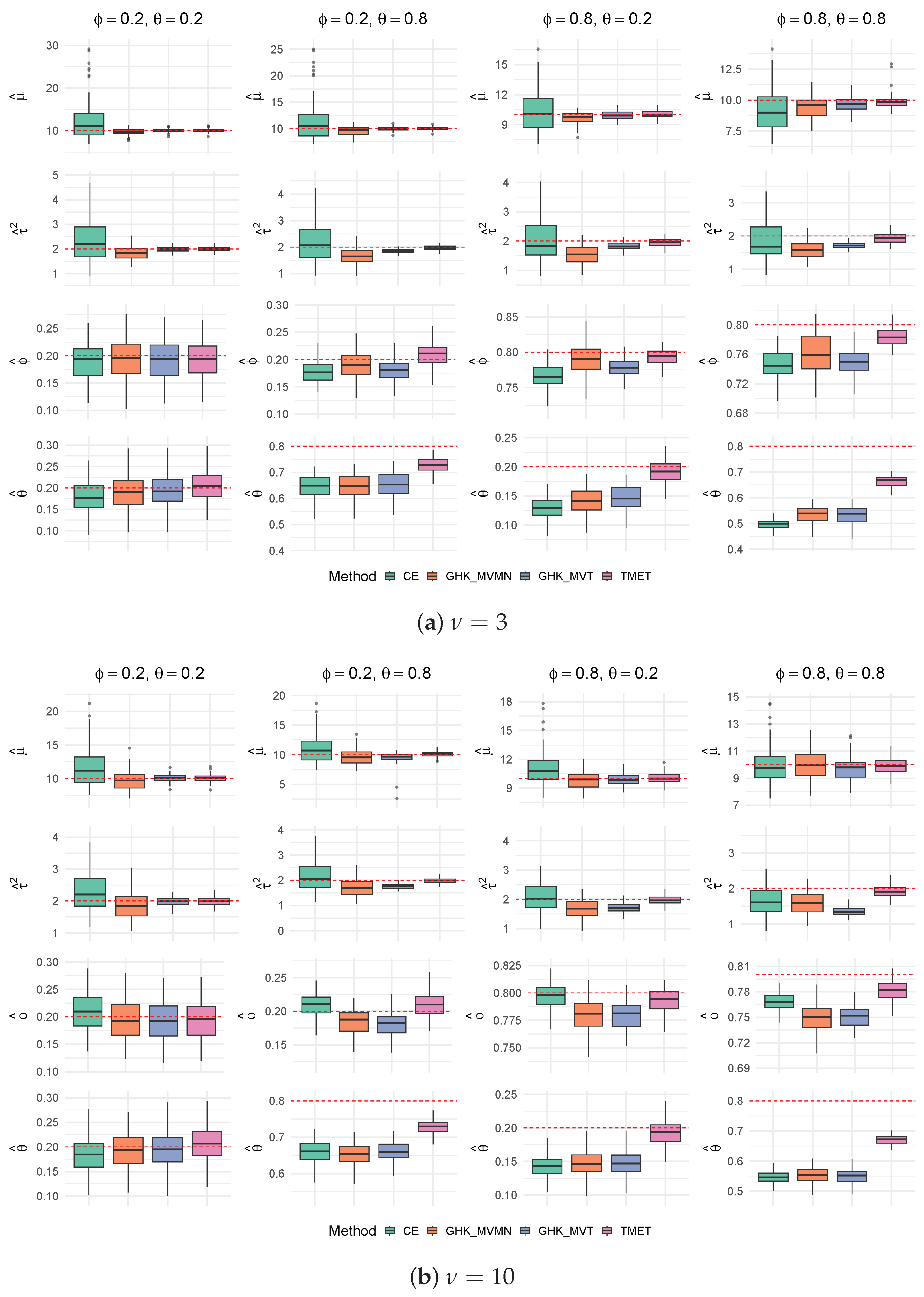
Sampling Distributions of MLEs. Figure A7, Figure A8, Figure A9, Figure A10, Figure A11 and Figure A12 summarize the sampling distributions of the maximum likelihood estimates based on each likelihood approximation with $n=5000$ observations. The qualitative patterns closely mirror those of the likelihood accuracy results. The CE approximation exhibits the largest bias and variability, particularly under heavy tails ($\nu =3$) or highly discrete marginals ($\mu =1$), with pronounced shrinkage of the dependence estimates toward zero. Both GHK variants perform reasonably well when $\mu =10$ and serial dependence is moderate, but under $\mu =1$ or strong serial dependence—especially when $\nu =3$—their sampling distributions become substantially more dispersed and display clear bias in the dependence parameters, reflecting importance-weight degeneracy. The TMET approximation yields the most concentrated sampling distributions across all models considered. The estimates $(\widehat{\mu },\widehat{\varphi },\widehat{\theta })$ remain tightly centered around the true values, with only modest inflation of variability as serial dependence strengthens.

Overall, the simulation results demonstrate that TMET achieves inferential accuracy comparable to that of MET at a fraction of MET’s computational cost. CE provides a fast deterministic approximation that performs relatively well under light tails and large means, but deteriorates sharply when the degree of discreteness or tail heaviness is severe. The two GHK variants behave adequately in moderate regimes, but their performance deteriorates under heavy-tailed latent dependence, strong serial correlation, or highly discrete marginals.

Results from additional simulations for models with negative binomial marginals and AR(1), MA(1), and ARMA(1,1) latent processes are reported in Figure A13, Figure A14 and Figure A15 in Appendix B, which yield the same substantive conclusions.

7. Inference and Forecasting

7.1. Confidence Intervals

Let $\widehat{\mathit{\eta }}=(\widehat{\mathit{\psi }},\widehat{\mathit{\vartheta }})$ denote the parameter estimate that maximizes the approximate log-likelihood $\ell \left(\mathit{\eta }\right)$ obtained using one of the methods considered, CE, GHK–MVMN, GHK–MVT or TMET. Uncertainty quantification for these estimates is based on the observed information matrix

$$\widehat{\mathcal{I}}\left(\widehat{\mathit{\eta }}\right)=-{\displaystyle \frac{{\partial }^2\ell \left(\mathit{\eta }\right)}{\partial \mathit{\eta }\partial {\mathit{\eta }}^{\top }}}{|}_{\mathit{\eta }=\widehat{\mathit{\eta }}}.$$

For smooth likelihoods, the inverse $\widehat{\mathcal{I}}{\left(\widehat{\mathit{\eta }}\right)}^{-1}$ consistently estimates the asymptotic variance matrix of $\widehat{\mathit{\eta }}$. In the present setting, the log-likelihood is evaluated using either a deterministic approximation (CE) or a simulation-based approximation (GHK or TMET). For the latter, evaluations of $\ell \left(\mathit{\eta }\right)$ are carried out using a fixed randomized QMC stream for all $\mathit{\eta }$, ensuring that the approximate log-likelihood is a smooth and deterministic function. This stabilization is essential during optimization: without a fixed randomization, the Hessian would vary across evaluations, making numerical differentiation unreliable.

Under Monte Carlo or quasi-Monte Carlo sampling, $\widehat{\mathit{\eta }}$  behaves as a pseudo–MLE. As $M\to \infty$, each of the simulation-based approximations converges uniformly to the exact log-likelihood, as shown in [35], Chapter 10, Section 10.5.1. Consequently, for sufficiently large M, the observed information matrix based on the approximate likelihood provides an accurate estimate of the asymptotic covariance of $\widehat{\mathit{\eta }}$.

In practice, the Hessian is obtained numerically by setting the argument hessian = TRUE in the R function optim.

Given a fixed QMC seed, the numerically evaluated Hessian is stable and requires no analytic derivatives. The estimated standard error of ${\widehat{\eta }}_j$ is the square root of the jth diagonal entry of $\widehat{\mathcal{I}}{\left(\widehat{\mathit{\eta }}\right)}^{-1}$, and the approximate $100(1-\alpha )\%$ Wald-type confidence interval for ${\eta }_j$ is

$${\widehat{\eta }}_j\pm z_{\alpha /2}\sqrt{{\left(\widehat{\mathcal{I}}{\left(\widehat{\mathit{\eta }}\right)}^{-1}\right)}_{jj}},$$

where $z_{\alpha /2}$ denotes the upper $\alpha /2$ quantile of the standard normal distribution.

7.2. Predictive Inference

We base predictive inference about future counts on the one-step-ahead plug-in predictive distribution $P(Y_{n+1}=y\mid \mathit{y};\widehat{\mathit{\eta }})$, $y\in {\mathbb{N}}_0$. Under the model (12), the observed counts arise as a deterministic function of the latent variables, so the predictive distribution is given by

$$P(Y_{n+1}=y\mid \mathit{y};\widehat{\mathit{\eta }})={\int }_{{\mathbb{R}}^n}P(Y_{n+1}=y\mid \mathit{v};\widehat{\mathit{\eta }})h(\mathit{v}\mid \mathit{y};\widehat{\mathit{\eta }})d\mathit{v},$$

(40)

where

$$h(\mathit{v}\mid \mathit{y};\widehat{\mathit{\eta }})={\displaystyle \frac{{\tau }_n(\mathit{v};\nu ,{\mathbf{\Psi }}_{\widehat{\mathit{\vartheta }}})}{P(\mathit{V}\in [\mathit{a},\mathit{b}];\widehat{\mathit{\eta }})}}{\mathbf{1}}_{[\mathit{a},\mathit{b}]}\left(\mathit{v}\right).$$

(41)

Also, since $\{Y_{n+1}=y\}$ and $\{{\widehat{a}}_{n+1}\left(y\right)<V_{n+1}\le {\widehat{b}}_{n+1}\left(y\right)\}$ are equivalent events, with ${\widehat{a}}_{n+1}\left(y\right)$ and ${\widehat{b}}_{n+1}\left(y\right)$ defined similarly to (14) with $\mathit{\psi }=\widehat{\mathit{\psi }}$, and 

$$\left(V_{n+1}\mid \mathit{v};\widehat{\mathit{\eta }}\right)\sim t_1\left(\nu +n,{\widehat{m}}_{n+1}\left(\mathit{v}\right),{\displaystyle \frac{\nu +\widehat{d}\left(\mathit{v}\right)}{\nu +n}}{\widehat{s}}_{n+1}^2\right),$$

with ${\widehat{m}}_{n+1}\left(\mathit{v}\right)$ and ${\widehat{s}}_{n+1}^2$ defined similarly in (19), and $\widehat{d}\left(\mathit{v}\right)$ computed by (27) with $\mathit{\vartheta }=\widehat{\mathit{\vartheta }}$, it follows that

$$\begin{array}{cc}\hfill & P(Y_{n+1}=y\mid \mathit{v};\widehat{\mathit{\eta }})\hfill \\ \hfill & =T\left({\displaystyle \frac{{\widehat{b}}_{n+1}\left(y\right)-{\widehat{m}}_{n+1}\left(\mathit{v}\right)}{\sqrt{\frac{\nu +\widehat{d}\left(\mathit{v}\right)}{\nu +n}}{\widehat{s}}_{n+1}}};\nu +n\right)-T\left({\displaystyle \frac{{\widehat{a}}_{n+1}\left(y\right)-{\widehat{m}}_{n+1}\left(\mathit{v}\right)}{\sqrt{\frac{\nu +\widehat{d}\left(\mathit{v}\right)}{\nu +n}}{\widehat{s}}_{n+1}}};\nu +n\right).\hfill \end{array}$$

Simulation from (41) is computationally expensive because it requires the costly evaluation of the normalizing constant $P(\mathit{V}\in [\mathit{a},\mathit{b}];\widehat{\mathit{\eta }})$. Instead, we approximate (40) using importance sampling based on (20). Drawing ${\mathit{V}}^{\left(1\right)},\dots ,{\mathit{V}}^{\left(M\right)}\sim g_{\widehat{\mathit{\eta }},\nu }^{\left(1\right)}$, the predictive probabilities in (40) are approximated by the self-normalized estimator

$$\begin{array}{cc}\hfill & \widehat{P}(Y_{n+1}=y\mid \mathit{y};\widehat{\mathit{\eta }})\hfill \\ \hfill & ={\displaystyle \frac{{\displaystyle \sum _{k=1}^M{\widehat{\omega }}_1^{\left(k\right)}\left[T\left(\frac{{\widehat{b}}_{n+1}\left(y\right)-{\widehat{m}}_{n+1}^{\left(k\right)}}{\sqrt{\frac{\nu +{\widehat{d}}^{\left(k\right)}}{\nu +n}}{\widehat{s}}_{n+1}};\nu +n\right)-T\left(\frac{{\widehat{a}}_{n+1}\left(y\right)-{\widehat{m}}_{n+1}^{\left(k\right)}}{\sqrt{\frac{\nu +{\widehat{d}}^{\left(k\right)}}{\nu +n}}{\widehat{s}}_{n+1}};\nu +n\right)\right]}}{{\displaystyle \sum _{k=1}^M{\widehat{\omega }}_1^{\left(k\right)}}}},\hfill \end{array}$$

(42)

where ${\widehat{\omega }}_1^{\left(k\right)}$ is the weight defined in (30) evaluated at ${\mathit{V}}^{\left(k\right)}$ and $\widehat{\mathit{\eta }}$, and ${\widehat{m}}_{n+1}^{\left(k\right)}$, ${\widehat{s}}_{n+1}$, and ${\widehat{d}}^{\left(k\right)}$ are defined analogously. This estimator does not require the evaluation of $P(\mathit{V}\in [\mathit{a},\mathit{b}];\widehat{\mathit{\eta }})$, since this factor cancels in the numerator and denominator of ${\widehat{\omega }}_1^{\left(k\right)}$. We use $g_{\widehat{\mathit{\eta }},\nu }^{\left(1\right)}\left(\mathit{v}\right)$ as the proposal density because it directly generates truncated Student-t latent paths, allowing the conditional moments and quadratic form computed via the Innovations algorithm to be reused without recomputation when evaluating the predictive distribution. This leads to a simpler implementation and lower per-sample overhead for one-step-ahead prediction.

We compute the estimated predictive probabilities (42) for $y=0,1,\dots ,y_{max}$, where $y_{max}:=\lfloor max\left(\mathit{y}\right)+3\mathrm{sd}\left(\mathit{y}\right)\rfloor .$ These probabilities are then used to construct predictive summaries, including the predictive mean, predictive variance, prediction intervals, the logarithmic score, and the continuous ranked probability score (CRPS), following [14].

Remark 7.

Predictive probabilities can also be approximated using importance sampling with proposal densities $g_{\widehat{\mathit{\eta }},\nu }^{\left(2\right)}(w,\mathit{z})$ or $g_{\widehat{\mathit{\eta }},\nu ,{\kappa }^{*},{\mathit{\delta }}^{*}}^{\left(3\right)}(w,\mathit{z})$. However, these proposals require transforming Gaussian latent paths to the Student-t scale and recomputing conditional moments, leading to a higher per-sample computational cost for prediction.

8. Model Diagnostics

Goodness-of-fit assessment in copula models with discrete marginals requires care, because the marginal distribution functions are step functions and ordinary residuals do not have approximately continuous and interpretable distributions under the true model. We therefore employ conditional randomized quantile residuals [36], which introduce uniform jittering within each discrete mass and then apply the appropriate quantile function of the latent copula distribution. Under correct model specification, these residuals behave approximately as an i.i.d. sample from the $t\left(\nu \right)$ distribution and can be assessed using standard tools such as Q–Q plots, PIT histograms, and autocorrelation diagnostics.

Proposition 3.

Let $\mathit{y}$ be the observed counts generated from model (12) with parameter $\mathit{\eta }$. For $t=1,\dots ,n$, define the randomized quantile residual as

$$e_t=T^{-1}\left(F_t(y_t-1\mid {\mathit{y}}_{<t};\mathit{\eta })+u_t\left[F_t(y_t\mid {\mathit{y}}_{<t};\mathit{\eta })-F_t(y_t-1\mid {\mathit{y}}_{<t};\mathit{\eta })\right];\nu \right),$$

(43)

where $u_1,\dots ,u_n\stackrel{\mathrm{i}.\mathrm{i}.\mathrm{d}.}{\sim }\mathrm{unif}[0,1]$, and $F_t(·\mid {\mathit{y}}_{<t};\mathit{\eta })$ is the conditional cdf of $Y_t$ given the past observations ${\mathit{y}}_{<t}$. Then, $e_1,\dots ,e_n\stackrel{\mathrm{i}.\mathrm{i}.\mathrm{d}.}{\sim }t\left(\nu \right)$.

As residuals, we use ${\left\{{\widehat{e}}_t\right\}}_{t=1}^n$, obtained by replacing $\mathit{\eta }$ with $\widehat{\mathit{\eta }}$ on the right-hand side of (43). For each $y\in {\mathbb{N}}_0$, the events $\{Y_t\le y\}$ and $\{Y_t\le y-1\}$ are equivalent to, respectively, $\{V_t\le b_t\left(y\right)\}$ and $\{V_t\le a_t\left(y\right)\}$, where $a_t\left(y\right),b_t\left(y\right)$ are defined as in (14). Thus, for $t=1,\dots ,n$, the estimated conditional cdfs can be written as

$$\begin{array}{cc}\hfill F_t(y_t\mid {\mathit{y}}_{<t};\widehat{\mathit{\eta }})& ={\int }_{{\mathbb{R}}^{t-1}}T\left({\displaystyle \frac{{\widehat{b}}_t\left(y_t\right)-{\widehat{m}}_t\left({\mathit{v}}_{<t}\right)}{\sqrt{\frac{\nu +\widehat{d}\left({\mathit{v}}_{<t}\right)}{\nu +t-1}}{\widehat{s}}_t}};\nu +t-1\right)h({\mathit{v}}_{<t}\mid {\mathit{y}}_{<t};\widehat{\mathit{\eta }})d{\mathit{v}}_{<t},\hfill \\ \hfill F_t(y_t-1\mid {\mathit{y}}_{<t};\widehat{\mathit{\eta }})& ={\int }_{{\mathbb{R}}^{t-1}}T\left({\displaystyle \frac{{\widehat{a}}_t\left(y_t\right)-{\widehat{m}}_t\left({\mathit{v}}_{<t}\right)}{\sqrt{\frac{\nu +\widehat{d}\left({\mathit{v}}_{<t}\right)}{\nu +t-1}}{\widehat{s}}_t}};\nu +t-1\right)h({\mathit{v}}_{<t}\mid {\mathit{y}}_{<t};\widehat{\mathit{\eta }})d{\mathit{v}}_{<t},\hfill \end{array}$$

where $h({\mathit{v}}_{<t}\mid {\mathit{y}}_{<t};\widehat{\mathit{\eta }})$ is the pdf of the $t_{t-1}(\nu ,\mathbf{0},{\mathbf{\Psi }}_{\widehat{\mathit{\vartheta }},<t})$ distribution truncated to $[{\widehat{\mathit{a}}}_{<t},{\widehat{\mathit{b}}}_{<t}]$, with ${\mathbf{\Psi }}_{\widehat{\mathit{\vartheta }},<t}$ the $(t-1)\times (t-1)$ leading principal submatrix of ${\mathbf{\Psi }}_{\widehat{\mathit{\vartheta }}}$, and 

$$[{\widehat{\mathit{a}}}_{<t},{\widehat{\mathit{b}}}_{<t}]:=\underset{i=1}{\overset{t-1}{⨂}}[{\widehat{a}}_i,{\widehat{b}}_i].$$

Like the predictive distribution (40), these conditional cdfs can be estimated by importance sampling using the proposal density $g_{\widehat{\mathit{\eta }},\nu }^{\left(1\right)}$, resulting in the estimators

$$\begin{array}{cc}\hfill {\widehat{F}}_t(y_t\mid {\mathit{y}}_{<t};\widehat{\mathit{\eta }})& ={\displaystyle \frac{{\displaystyle \sum _{k=1}^M{\widehat{\omega }}_{1,t}^{\left(k\right)}T\left(\frac{{\widehat{b}}_t\left(y_t\right)-{\widehat{m}}_t\left({\mathit{V}}_{<t}^{\left(k\right)}\right)}{\sqrt{\frac{\nu +\widehat{d}\left({\mathit{V}}_{<t}^{\left(k\right)}\right)}{\nu +t-1}}{\widehat{s}}_t};\nu +t-1\right)}}{{\displaystyle \sum _{k=1}^M{\widehat{\omega }}_{1,t}^{\left(k\right)}}}},\hfill \\ \hfill {\widehat{F}}_t(y_t-1\mid {\mathit{y}}_{<t};\widehat{\mathit{\eta }})& ={\displaystyle \frac{{\displaystyle \sum _{k=1}^M{\widehat{\omega }}_{1,t}^{\left(k\right)}T\left(\frac{{\widehat{a}}_t\left(y_t\right)-{\widehat{m}}_t\left({\mathit{V}}_{<t}^{\left(k\right)}\right)}{\sqrt{\frac{\nu +\widehat{d}\left({\mathit{V}}_{<t}^{\left(k\right)}\right)}{\nu +t-1}}{\widehat{s}}_t};\nu +t-1\right)}}{{\displaystyle \sum _{k=1}^M{\widehat{\omega }}_{1,t}^{\left(k\right)}}}}.\hfill \end{array}$$

Here, ${\mathit{V}}^{\left(1\right)},\dots ,{\mathit{V}}^{\left(M\right)}\stackrel{\mathrm{i}.\mathrm{i}.\mathrm{d}.}{\sim }{g}_{\widehat{\mathit{\eta }},\nu }^{\left(1\right)}$ and the importance weights are given by

$$\begin{array}{cc}\hfill {\widehat{\omega }}_{1,t}^{\left(k\right)}& ={\displaystyle \frac{{\tau }_{t-1}({\mathit{V}}_{<t}^{\left(k\right)};\nu ,{\mathbf{\Psi }}_{\widehat{\mathit{\vartheta }},<t})}{g_{\widehat{\mathit{\eta }},\nu ,t-1}^{\left(1\right)}\left({\mathit{V}}_{<t}^{\left(k\right)}\right)}}\hfill \\ \hfill & =\prod _{i=1}^{t-1}\left[T\left({\displaystyle \frac{{\widehat{b}}_i\left(y_i\right)-{\widehat{m}}_i\left({\mathit{V}}_{<i}^{\left(k\right)}\right)}{\sqrt{\frac{\nu +\widehat{d}\left({\mathit{V}}_{<i}^{\left(k\right)}\right)}{\nu +i-1}}{\widehat{s}}_i}};\nu +i-1\right)-T\left({\displaystyle \frac{{\widehat{a}}_i\left(y_i\right)-{\widehat{m}}_i\left({\mathit{V}}_{<i}^{\left(k\right)}\right)}{\sqrt{\frac{\nu +\widehat{d}\left({\mathit{V}}_{<i}^{\left(k\right)}\right)}{\nu +i-1}}{\widehat{s}}_i}};\nu +i-1\right)\right],\hfill \end{array}$$

where ${\widehat{a}}_i\left(y_i\right)$ and ${\widehat{b}}_i\left(y_i\right)$ are defined as in (14) with $\mathit{\psi }$ replaced by $\widehat{\mathit{\psi }}$, ${\mathit{V}}_{<t}^{\left(k\right)}$ is the vector formed by the first $t-1$ components of ${\mathit{V}}^{\left(k\right)}$, and 

$$g_{\widehat{\mathit{\eta }},\nu ,t-1}^{\left(1\right)}\left({\mathit{V}}_{<t}^{\left(k\right)}\right)=\prod _{i=1}^{t-1}h(v_i\mid {\mathit{v}}_{<i},y_i;\nu ,{\mathbf{\Psi }}_{\widehat{\mathit{\vartheta }}}).$$

These residuals can then be assessed using standard diagnostic tools such as Q–Q plots, PIT histograms, and autocorrelation functions. These are illustrated in the next section.

9. An Application

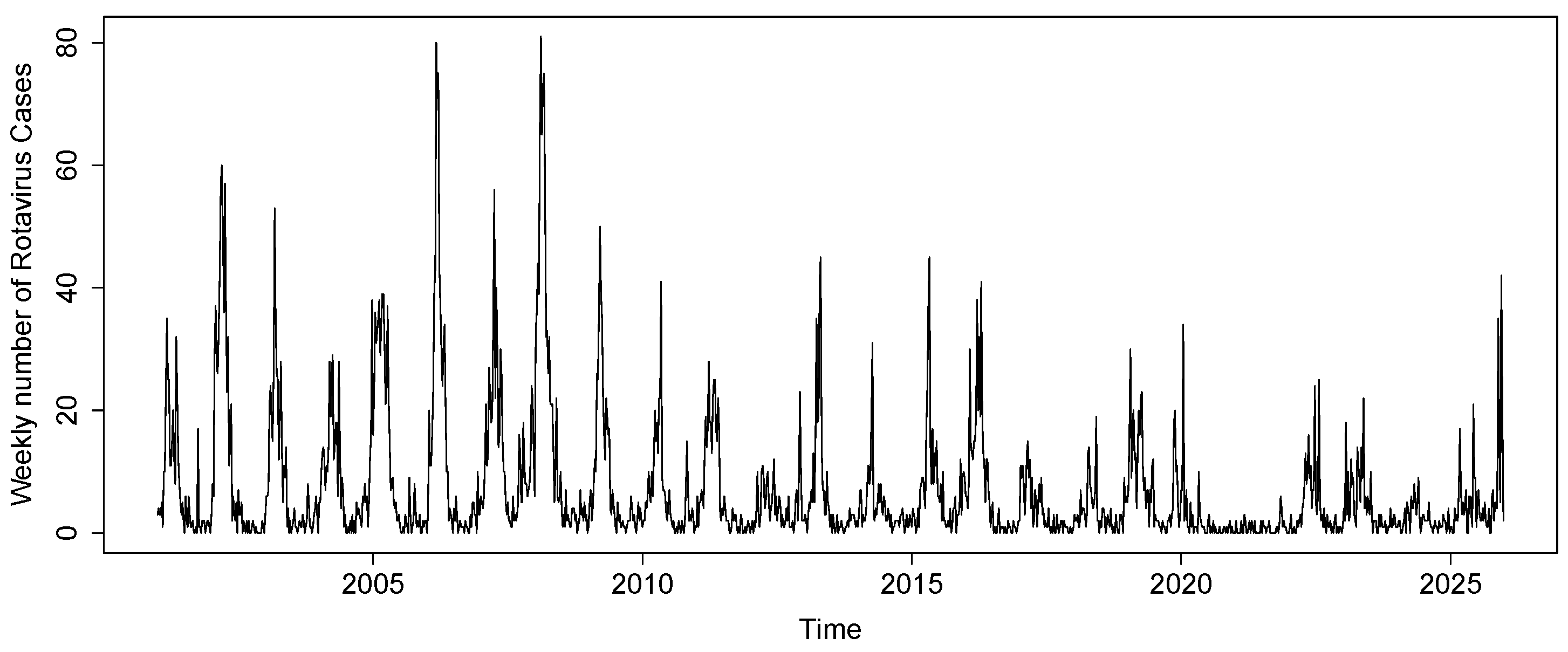
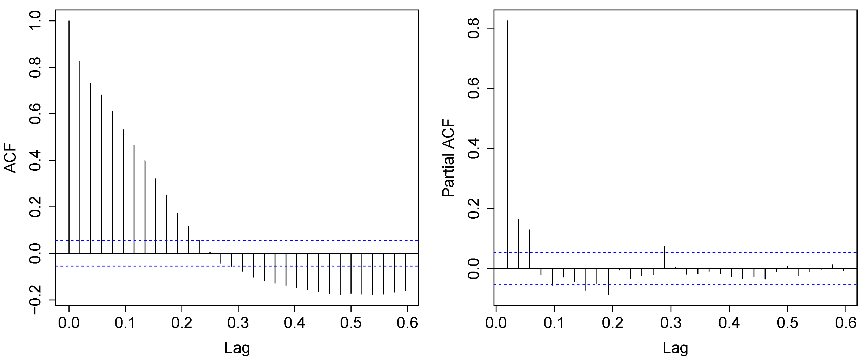
To illustrate the proposed likelihood framework and examine its empirical behavior in a real epidemiological time series, we analyze weekly counts of rotavirus gastroenteritis reported to the Robert Koch Institute (RKI) in Germany. Rotavirus is a highly contagious virus that primarily affects young children and can cause severe diarrhea and dehydration. The complete dataset spans 2001–2025 (approximately 1300 weeks) across 412 urban districts in Germany; here we focus on the time series from Meiben County. The series is divided into a training set of 1000 weeks and a testing set of 300 weeks. Figure 3 displays the observed counts, revealing pronounced seasonal variation. The sample ACF and PACF plots in Figure 4 further indicate persistent serial dependence with seasonal structure.

Since the sample variance (117.604) substantially exceeds the sample mean (7.197), we adopt negative binomial marginals with mean function ${\mu }_t$ and overdispersion parameter ${\tau }^2$. After exploratory analysis, seasonality is modeled through the mean function

$${\mu }_t=exp\left({\beta }_0+{\beta }_{1}sin\left({\displaystyle \frac{2\pi }{52}}t\right)+{\beta }_{2}cos\left({\displaystyle \frac{2\pi }{52}}t\right)+{\beta }_{3}sin\left({\displaystyle \frac{4\pi }{52}}t\right)+{\beta }_{4}cos\left({\displaystyle \frac{4\pi }{52}}t\right)\right).$$

Based on the autocorrelation diagnostics and residual analysis from preliminary models, a t–ARMA(1,1) process is selected for the latent dependence structure. The parameter vector is then $\mathit{\eta }=({\beta }_0,{\beta }_1,{\beta }_2,{\beta }_3,{\beta }_4,{\tau }^2,\varphi ,\theta )$. Maximum likelihood estimation is performed using the proposed TMET approximation. Initial values for the marginal parameters are obtained from negative binomial GLM fits, while the dependence parameters are initialized from ARMA fits to the observed series.

For the Student-t copula, we examine degrees of freedom $\nu \in \{5,10,20,30,50\}$.

Table 1. Kolmogorov–Smirnov distance of PIT values from the $\mathrm{unif}(0,1)$ distribution for different degrees of freedom $\nu$.

$\mathit{\nu }$	5	10	20	30	50
KS statistic	0.0637	0.0541	0.0527	0.0524	0.0480

reports the Kolmogorov–Smirnov (KS) distance between the PIT values and the $\mathrm{unif}[0,1]$ distribution. The KS statistics are similar across values of $\nu$ and decrease mildly as $\nu$ increases, indicating that the latent tail parameter is only weakly identifiable in this dataset and that the evidence for pronounced tail dependence is limited. As $\nu$ increases, the Student-t copula approaches the Gaussian copula. Accordingly, we adopt $\nu =50$, which yields the smallest KS statistic among the values considered.

Table 2. MLEs of the copula model parameters under Gaussian and Student-t copulas (ARMA(1,1) dependence, negative binomial marginals).

	Gaussian Copula			Student-t Copula ($\mathit{\nu }=50$)
Parameter	Estimate	Sth. Error	Pr (>|z|)	Estimate	Sth. Error	Pr (>|z|)
${\beta }_0$	1.798	0.094	<2 × 10−16	1.867	0.100	<2 × 10−16
${\beta }_1$	0.884	0.093	<2 × 10−16	0.840	0.091	<2 × 10−16
${\beta }_2$	0.222	0.080	0.00546	0.241	0.079	0.00211
${\beta }_3$	$-0.128$	0.060	0.03353	$-0.127$	0.059	0.03203
${\beta }_4$	$-0.204$	0.060	0.00067	$-0.201$	0.059	0.00062
${\tau }^2$	0.618	0.080	$9.62\times {10}^{-15}$	0.698	0.148	$2.26\times {10}^{-6}$
$\varphi$	0.884	0.024	<2 × 10−16	0.889	0.023	<2 × 10−16
$\theta$	$-0.485$	0.047	<2 × 10−16	$-0.485$	0.046	<2 × 10−16
Log-lik	$-2591.28$			$-2593.82$
AIC	5198.56			5203.64
BIC	5237.82			5242.91

compares maximum likelihood estimates under Gaussian and Student-t copulas. The parameter estimates and standard errors are quite close under the two specifications. Information criteria show negligible differences between the two models, consistent with the weak sensitivity of the fit to the tail index $\nu$ observed in Table 1. This behavior illustrates an important property of the proposed framework: when tail dependence is weak, the Student-t copula naturally approaches the Gaussian copula as a limiting case. Thus, the t copula provides a flexible generalization without sacrificing stability when heavy tails are absent.

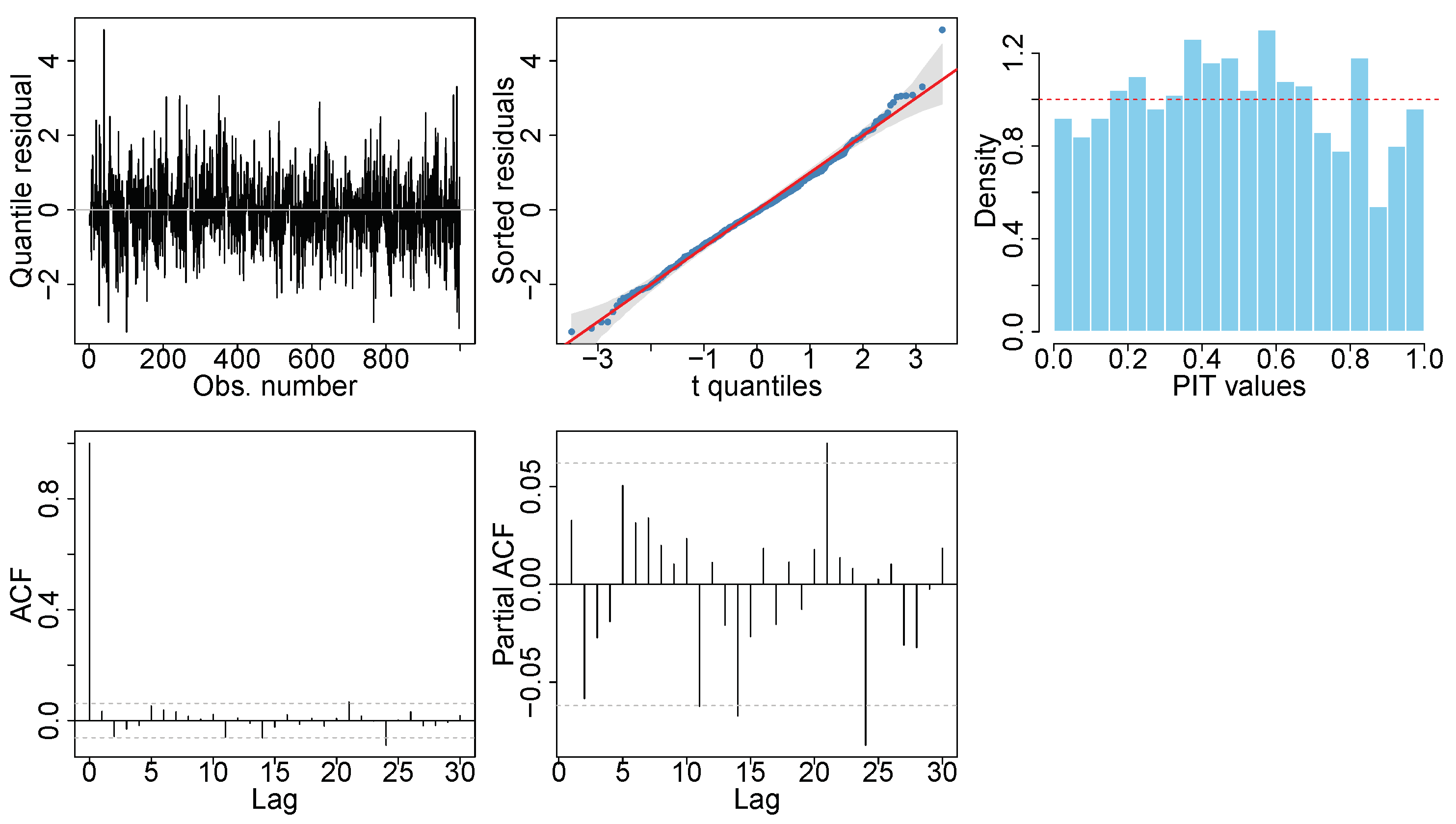
The residual diagnostics displayed in Figure 5 show that the transformed quantile residuals fluctuate around zero without visible structure. The Q–Q plot aligns closely with the reference t distribution, with only a minor deviation in the upper tail. The PIT histogram is approximately uniform, and the residual ACF and PACF reveal no significant remaining serial dependence. Overall, these diagnostics indicate an adequate fit with no clear evidence of model misspecification.

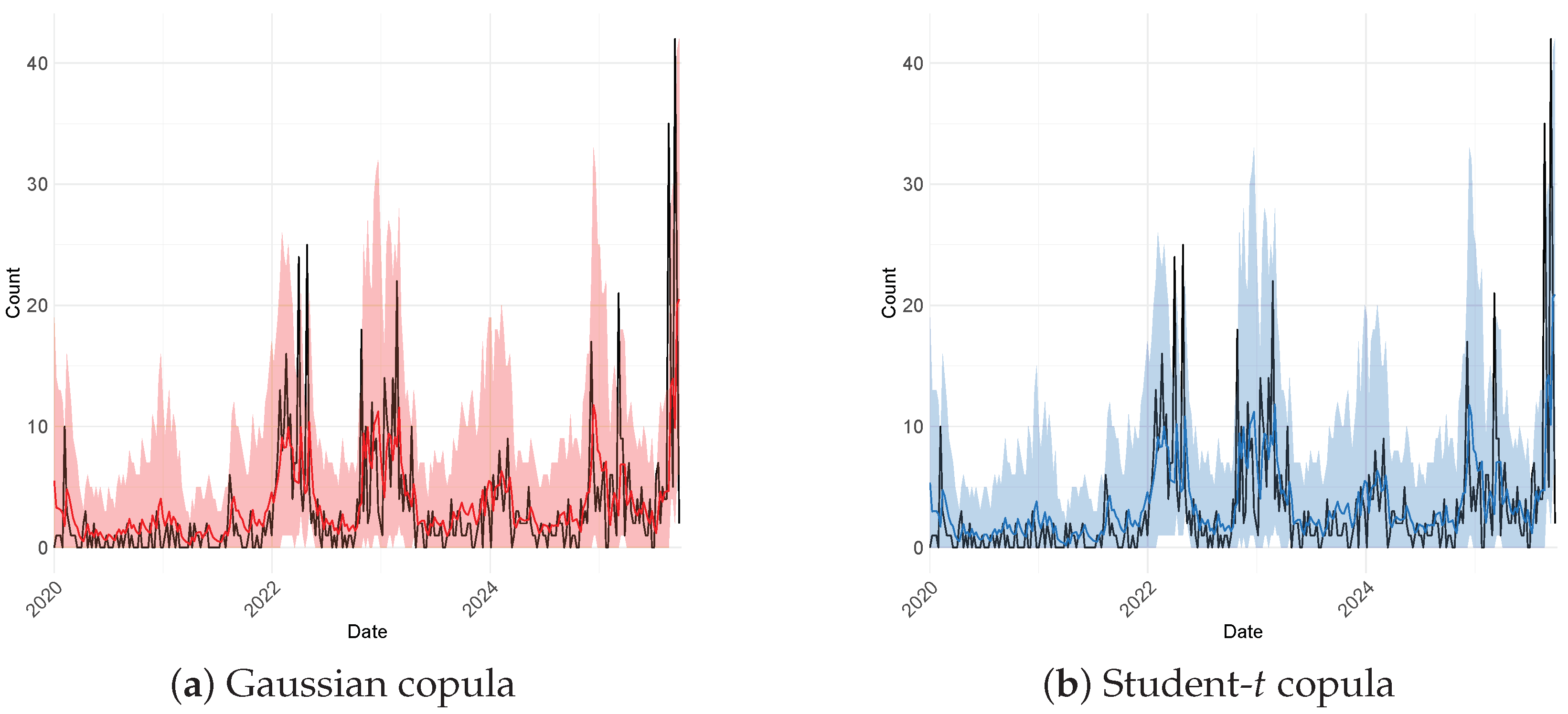
The predictive performance on the testing set, reported in

Table 3. Predictive performance of Student-t and Gaussian copula models for the test sample.

Method	MSPE	CRPS a	LOGS a	Coverage	Sharpness
Student-t Copula	19.604	0.507	0.493	0.97	11.123
Gaussian Copula	19.623	–	–	0.97	11.023

^a Proportion of test cases in which the Student-t copula yields lower CRPS (or LOGS) than the Gaussian copula.

, indicates that the one-step-ahead forecasts under the Gaussian and Student-t copulas are nearly indistinguishable. The mean squared prediction errors are essentially identical, and both models achieve comparable coverage rates of approximately 97%. The average interval widths (sharpness) are also very similar. In terms of distributional scores, the Student-t copula yields lower CRPS and LOGS values in approximately half of the test observations (0.507 and 0.493, respectively), indicating that the two specifications perform similarly in probabilistic forecasting. As illustrated in Figure 6, the predictive means track the observed seasonal dynamics closely under both models, and the associated prediction intervals behave similarly. Additional fits using alternative values of $\nu$ produce nearly identical forecasting summaries. Taken together, these results suggest that, for this dataset, short-horizon predictive performance is largely insensitive to the choice of degrees of freedom.

This application highlights a practical feature of the proposed framework: when heavy-tailed dependence is weak or not supported by the data, the Student-t copula naturally approaches the Gaussian specification, offering a flexible extension that adapts to the degree of tail heaviness while preserving stable inference.

10. Conclusions

This paper develops a scalable likelihood-based framework for count time series modeled through a Student-t copula with latent ARMA dependence. A central contribution is the integration of an explicit time-domain construction of a latent t–ARMA process with a likelihood approximation strategy that exploits its exact conditional structure. By combining the scale-mixture representation of the multivariate t distribution with the linear recursions of the Innovations algorithm, we formulate a time series version of minimax exponential tilting (TMET) tailored to heavy-tailed copula models. The resulting procedure preserves the near-linear computational footprint previously achieved in the Gaussian setting while targeting the more demanding heavy-tailed likelihood.

Through extensive simulation experiments, we compared TMET with extensions of the continuous extension (CE) and Geweke–Hajivassiliou–Keane (GHK) approximations to the Student-t copula setting. Across a broad range of dependence strengths, marginal degrees of discreteness, and tail indices, TMET consistently provided the most accurate and numerically stable likelihood approximation. The CE and GHK methods remained competitive in some settings, but exhibited increased variability or bias under strong serial dependence and small degrees of freedom. These findings establish TMET as a reliable and scalable likelihood tool for heavy-tailed copula time series.

The proposed framework also supports standard likelihood-based inference and prediction. The observed Fisher information yields standard errors directly, and one-step-ahead predictive distributions can be computed using self-normalized importance sampling based on the same proposal densities used for likelihood evaluation. In the real data application, the Student-t copula approaches the Gaussian copula as a limiting case, and the empirical results illustrate that, in moderate samples, the tail index may be only weakly identifiable. This reinforces the interpretation of the t copula as a flexible generalization rather than a replacement for Gaussian copula models.

An important direction for future research is the extension of the proposed framework to asymmetric Student-t copula constructions, which would allow asymmetric tail dependence and broaden the scope of the proposed methodology; see [37] and the references therein. Such an extension would be of considerable practical interest and merit further investigation. Another important direction includes the extension to multivariate count time series, where modeling cross-sectional dependence and joint extremal behavior would further broaden the applicability of the proposed framework. Another important direction concerns estimation of the degrees-of-freedom parameter. While in this work we examine a grid of fixed values to assess tail sensitivity, developing stable and theoretically grounded procedures for joint estimation of $\nu$ remains an open problem, particularly given the weak identifiability of tail parameters in discrete settings. The accompanying gctsc R package provides scalable tools for likelihood inference and forecasting in long time series and offers a foundation for continued methodological development and applied research in heavy-tailed copula models.

References

1. Patton, A.J. A review of copula models for economic time series. J. Multivar. Anal. 2012, 110, 4–18. [Google Scholar] [CrossRef] [Scilit]
2. Masarotto, G.; Varin, C. Gaussian copula marginal regression. Electron. J. Stat. 2012, 6, 1517–1549. [Google Scholar] [CrossRef] [Scilit]
3. Han, Z.; De Oliveira, V. Maximum likelihood estimation of Gaussian copula models for geostatistical count data. Commun. Stat. Simul. Comput. 2020, 49, 1957–1981. [Google Scholar] [CrossRef] [Scilit]
4. Jia, Y.; Kechagias, S.; Livsey, J.; Lund, R.; Pipiras, V. Latent Gaussian count time series. J. Am. Stat. Assoc. 2023, 118, 596–606. [Google Scholar] [CrossRef] [Scilit]
5. Xu, N.; Yang, K. High-dimensional and banded integer-valued autoregressive processes. Comput. Stat. Data Anal. 2025, 212, 108243. [Google Scholar] [CrossRef] [Scilit]
6. Sheng, D.; Wang, D.; Sun, L. A new first-order mixture integer-valued threshold autoregressive process based on binomial thinning and negative binomial thinning. J. Stat. Plan. Inference 2024, 231, 106143. [Google Scholar] [CrossRef] [Scilit]
7. Joe, H. Dependence Modeling with Copulas; CRC Press: Boca Raton, FL, USA, 2014. [Google Scholar]
8. Demarta, S.; McNeil, A.J. The t copula and related copulas. Int. Stat. Rev. 2005, 73, 111–129. [Google Scholar] [CrossRef] [Scilit]
9. Breymann, W.; Dias, A.; Embrechts, P. Dependence structures for multivariate high–frequency data in finance. Quant. Financ. 2003, 3, 1. [Google Scholar] [CrossRef]
10. Oh, D.H.; Patton, A.J. Modeling dependence in high dimensions with factor copulas. J. Bus. Econ. Stat. 2017, 35, 139–154. [Google Scholar] [CrossRef] [Scilit]
11. Genz, A.; Bretz, F. Computation of Multivariate Normal and t Probabilities; Springer: Berlin/Heidelberg, Germany, 2009. [Google Scholar]
12. Botev, Z.I.; L’Ecuyer, P. Efficient probability estimation and simulation of the truncated multivariate Student–t distribution. In Proceedings of the 2015 Winter Simulation Conference (WSC); IEEE: New York, NY, USA, 2015; pp. 380–391. [Google Scholar]
13. Cao, J.; Katzfuss, M. Linear–cost Vecchia approximation of multivariate normal probabilities. J. Am. Stat. Assoc. 2026; in press. [CrossRef] [Scilit]
14. Nguyen, Q.N.; De Oliveira, V. Likelihood inference in Gaussian copula models for count time series via minimax exponential tilting. Comput. Stat. Data Anal. 2026, 218, 108344. [Google Scholar] [CrossRef] [Scilit]
15. Masarotto, G.; Varin, C. Gaussian copula regression in R. J. Stat. Softw. 2017, 77, 1–26. [Google Scholar] [CrossRef] [Scilit]
16. Han, Z.; De Oliveira, V. gckrig: An R package for the analysis of geostatistical count data using Gaussian copulas. J. Stat. Softw. 2018, 87, 1–32. [Google Scholar] [CrossRef] [Scilit]
17. Nadarajah, S.; Kotz, S. Mathematical properties of the multivariate t distribution. Acta Appl. Math. 2005, 89, 53–84. [Google Scholar] [CrossRef] [Scilit]
18. Ding, P. On the conditional distribution of the multivariate t distribution. Am. Stat. 2016, 70, 293–295. [Google Scholar] [CrossRef] [Scilit]
19. Shah, A.; Wilson, A.G.; Ghahramani, Z. Student–t processes as alternatives to Gaussian processes. In Proceedings of the 17th International Conference on Artificial Intelligence and Statistics (AISTATS), Reykjavik, Iceland, 22–25 April 2014; Volume 33. [Google Scholar]
20. Meitz, M.; Preve, D.; Saikkonen, P. A mixture autoregressive model based on Student’s t-distribution. Commun. Stat. Theory Methods 2023, 52, 498–514. [Google Scholar] [CrossRef] [Scilit]
21. Nelsen, R.B. An Introduction to Copulas, 2nd ed.; Springer: Berlin/Heidelberg, Germany, 2006. [Google Scholar]
22. Song, P.X. Multivariate dispersion models generated from Gaussian copula. Scand. J. Stat. 2000, 27, 305–320. [Google Scholar] [CrossRef] [Scilit]
23. Brockwell, P.J.; Davis, R.A. Introduction to Time Series and Forecasting, 3rd ed.; Springer: Berlin/Heidelberg, Germany, 2016. [Google Scholar]
24. Han, Z.; De Oliveira, V. On the correlation structure of Gaussian copula models for geostatistical count data. Aust. N. Z. J. Stat. 2016, 58, 47–69. [Google Scholar] [CrossRef] [Scilit]
25. Geweke, J. Efficient simulation from the multivariate normal and Student–t distributions subject to linear constraints and the evaluation of constraint probabilities. In Computing Science and Statistics: Proceedings of the 23rd Symposium on the Interface; Interface Foundation of North America: Fairfax Station, VA, USA, 1991; pp. 571–578. [Google Scholar]
26. Hajivassiliou, V.; McFadden, D.; Ruud, P. Simulation of multivariate normal rectangle probabilities and their derivatives: Theoretical and computational results. J. Econom. 1996, 72, 85–134. [Google Scholar] [CrossRef] [Scilit]
27. Keane, M.P. A computationally practical simulation estimator for panel data. Econometrica 1994, 62, 95–116. [Google Scholar] [CrossRef] [Scilit]
28. Genz, A.; Bretz, F. Numerical computation of multivariate t probabilities with application to power calculation of multiple contrasts. J. Stat. Comput. Simul. 1999, 63, 103–117. [Google Scholar] [CrossRef] [Scilit]
29. Cao, J.; Genton, M.G.; Keyes, D.E.; Turkiyyah, G.M. Exploiting low–rank covariance structures for computing high–dimensional normal and Student–t probabilities. Stat. Comput. 2021, 31, 2. [Google Scholar] [CrossRef] [Scilit]
30. Kazianka, H.; Pilz, J. Copula–based geostatistical modeling of continuous and discrete data including covariates. Stoch. Environ. Res. Risk Assess. 2010, 24, 661–673. [Google Scholar] [CrossRef] [Scilit]
31. Nguyen, Q.N.; De Oliveira, V. Approximating Gaussian copula models for count time series: Connecting the distributional transform and a continuous extension. J. Appl. Stat. 2026, 53, 1–22. [Google Scholar] [CrossRef] [Scilit]
32. Botev, Z.I. The normal law under linear restrictions: Simulation and estimation via minimax tilting. J. R. Stat. Soc. Ser. B 2017, 79, 125–148. [Google Scholar] [CrossRef] [Scilit]
33. Madsen, K.; Nielsen, H.B.; Tingleff, O. Methods for Non-Linear Least Squares Problems; Technical University of Denmark: Kongens Lyngby, Denmark, 2014. [Google Scholar]
34. Golub, G.H.; Van Loan, C.F. Matrix Computations, 4th ed.; Johns Hopkins University Press: Baltimore, MD, USA, 2013. [Google Scholar]
35. Train, K.E. Discrete Choice Methods with Simulation; Cambridge University Press: Cambridge, UK, 2009. [Google Scholar]
36. Dunn, P.K.; Smyth, G.K. Randomized quantile residuals. J. Comput. Graph. Stat. 1996, 5, 236–244. [Google Scholar] [CrossRef] [Scilit]
37. Deng, L.; Smith, M.S.; Maneesoonthorn, W. Large skew-t copula models and asymmetric dependence in intraday equity returns. J. Bus. Econ. Stat. 2025, 43, 269–285. [Google Scholar] [CrossRef] [Scilit]
38. Prékopa, A. On logarithmic concave measures and functions. Acta Sci. Math. 1973, 34, 335–343. [Google Scholar]
Figure 1. Histograms of importance sampling weights ω 2 in (30) (relative to their maximum) for the GHK and TMET estimators with Poisson marginals ( μ { 1 , 10 } ) and AR(1) latent processes ( ϕ { 0.2 , 0.9 } ); n = 30 and M = 1000 . (a) GHK; (b) TMET.
Stats 09 00043 g001
Figure 2. Samples drawn from the GHK (left) and TMET (right) proposals for a Poisson–AR(1) model with mean μ = 1 and correlation ϕ = 0.9 (red dots). The blue contours represent the bivariate t density, and the black box indicates the truncation region corresponding to the observed counts y = ( 0 , 1 ) .
Stats 09 00043 g002
Figure 3. Weekly number of rotavirus cases in Meissen County, Germany, 2001–2025.
Stats 09 00043 g003
Figure 4. Sample ACF and PACF plots for the weekly rotavirus counts.
Stats 09 00043 g004
Figure 5. Residual plots for the Student-t copula model fitted to the rotavirus training data, computed using the TMET method.
Stats 09 00043 g005
Figure 6. Rotavirus testing data and one-step-ahead forecasts. Black line: observed counts; blue/red lines: predictive means; and shaded bands: 95% predictive intervals. Panels (a) and (b) correspond to Gaussian and Student-t copula models, respectively.
Stats 09 00043 g006